Robust uncertainty estimates with out-of-distribution pseudo-inputs training
Pierre Segonne Yevgen Zainchkovskyy Søren Hauberg
pierre.segonne@electricitymap.org yeza@dtu.dk sohau@dtu.dk
Abstract
Probabilistic models often use neural networks to control their predictive uncertainty. However, when making out-of-distribution (OOD) predictions, the often-uncontrollable extrapolation properties of neural networks yield poor uncertainty predictions. Such models then don’t know what they don’t know, which directly limits their robustness w.r.t unexpected inputs. To counter this, we propose to explicitly train the uncertainty predictor where we are not given data to make it reliable. As one cannot train without data, we provide mechanisms for generating pseudo-inputs in informative low-density regions of the input space, and show how to leverage these in a practical Bayesian framework that casts a prior distribution over the model uncertainty. With a holistic evaluation, we demonstrate that this yields robust and interpretable predictions of uncertainty while retaining state-of-the-art performance on diverse tasks such as regression and generative modelling.
1 Introduction
Neural networks generally extrapolate arbitrarily (Xu et al. 2020), and high quality predictions are limited to regions of the input space where the networks have been trained. This is to be expected and is only problematic if the associated predictions are not accompanied with a well-calibrated measure of uncertainty. If a neural network is used for estimating such a measure of uncertainty, we, however, quickly run into trouble, as the reported uncertainty then exhibits arbitrary behaviour in regions with no training data. Alarmingly, these are exactly the regions where evaluating the uncertainty is most important to the safe deployment of machine learning models in real world applications (Amodei et al. 2016). One potential solution is to avoid using directly the output of neural networks for predicting uncertainty, and let it emerge from another mechanism, e.g. an ensemble (Hansen and Salamon 1990; Lakshminarayanan et al. 2017) or some notion of Monte Carlo (MacKay 1992; Gal and Ghahramani 2016). Here we explore the alternative view that the networks should simply be trained where there is no data.
But can we train without data? The Bayesian formalism often does so implicitly: most conjugate priors can be seen as additional training data (Bishop 2006), e.g. in Gaussian models, a mean prior can be realised by additional training data of with setting the amount of observations. Placing a prior over the output of a neural network can, thus, be interpreted as additional training data. Unfortunately, this view is not practical as it implies additional data for all possible inputs to a neural network, resulting in infinite data. Our approach is simple: we locate regions of low data density in input space and implicitly place observations here in output space by minimising an appropriate KL divergence towards a prior (see Fig. 1). The result is a simple algorithm that significantly improves uncertainty estimates in both regression and generative modeling.
1.1 Background and related work
The predictive performance of machine learning models has drastically increased in the past decade, but the quality of the accompanying uncertainties have not followed. Uncertainties are reported as being miscalibrated (Guo et al. 2017) and overconfident (Lakshminarayanan et al. 2017; Hendrycks and Gimpel 2016). Some models even see higher likelihoods of out-of-distribution than in-distribution data (Nalisnick et al. 2019; Nguyen et al. 2015; Louizos and Welling 2017).
Neural networks commonly output distributions which gives a notion of predictive uncertainty. Classifiers trained with soft-max is an ever-present example of such. These predictions are generally observed to be overconfident (Lakshminarayanan et al. 2017; Hendrycks and Gimpel 2016) and to carry little meaning outside the support of the training data (Skafte et al. 2019; Lee et al. 2017). The latter is an artifact of the hard-to-control extrapolation that comes with neural networks (Xu et al. 2021). In general, since extrapolation is difficult to control, uncertainties predicted by neural networks will exhibit seemingly arbitrary behavior outside the support of the data, yielding untrustworthy results.
Mean-variance networks for regression (Nix and Weigend 1994) model the conditional target density as a Gaussian with mean and variance predicted by neural networks. The predictive uncertainty is generally accurate in regions near training data, but otherwise unreliable (Hauberg 2019). To counter this, Arvanitidis et al. 2017 and Skafte et al. 2019 proposed variance network architectures to enforce a specified extrapolation value, but these heuristics tend to be difficult to tune, and lack principle. Mean-variance networks have seen a recent uptake within generative modeling, where they are used as an encoder distribution in variational autoencoders (VAEs) (Kingma and Welling 2013; Rezende et al. 2014).
Which uncertainty? A commonly called-upon dichotomy (Der Kiureghian and Ditlevsen 2009) is that the uncertainty of a model’s prediction can be decomposed into the uncertainty of the model (epistemic) and of the data (aleatoric). The epistemic uncertainty can be lowered by increasing the amount of data, simplifying the model or otherwise reducing the complexity of the learning problem. The aleatoric uncertainty, on the other hand, is a property of the world, and cannot be changed; no prediction should ever be more certain than the uncertainty displayed by the associated data.
Bayesian methods are often used to quantify uncertainty due to their explicit formulation of uncertainty. Gaussian processes (GPs) (Rasmussen and Williams 2005) provide an elegant framework that provide state-of-the-art uncertainty estimates, but, alas, the corresponding mean predictions are often not up to the standards of neural networks. GPs are tightly linked to Bayesian neural networks (BNNs) (MacKay 1992) that place a prior over the network weights and seek the corresponding posterior. Despite advances in variational approximations (Graves 2011; Kingma and Welling 2013; Blundell et al. 2015), expectation propagation (Hernández-Lobato and Adams 2015; Hasenclever et al. 2017), or Monte Carlo methods (Welling and Teh 2011; Springenberg et al. 2016), training BNNs remains difficult. Furthermore, the predictive uncertainty seems dependent on the degree of approximation and is thus controlled by the available compute power.
Ensemble methods have long been used to produce aggregated predictions with uncertainty estimates (Hansen and Salamon 1990; Breiman 1996). Deep ensembles (Lakshminarayanan et al. 2017), a collection of differently initialized networks trained on the same data, are generally reported as state-of-the-art for uncertainty quantification in deep models (Thagaard et al. 2020; Ovadia et al. 2019). As the models in the ensemble are trained on overlapping data, they are correlated, which influence the ensemble uncertainty in ways that remains unclear (Breiman 2001). Monte-Carlo dropout (Gal and Ghahramani 2016) casts dropout training (Srivastava et al. 2014) as an ensemble model. It is computationally cheap, but experiments (Ovadia et al. 2019; Skafte et al. 2019) show that the increased correlation of ensemble elements causes overconfidence.
Robustness to distribution shift is part of a well-behaved uncertainty predictor (Ovadia et al. 2019) and must be evaluated accordingly. For out-of-distribution detection, Liang et al. 2017 proposes a pre-processing perturbation step inspired by adversarial attacks (Goodfellow et al. 2014a) that helps distinguish in-distribution and out-of-distribution inputs. Hendrycks et al. 2018 used a Generative Adversarial Network (GAN) (Goodfellow et al. 2014b) to generate out-of-distribution pseudo-inputs that appear in a regularizing term in the loss function, called outlier exposure, to enhance the predictor’s ability to discriminate out-of-distribution inputs (Lee et al. 2017; Dai et al. 2017).
Out-of-distribution pseudo-inputs can improve uncertainty estimates. Deep ensembles trained to maximise diversity on such pseudo-inputs can display high uncertainty outside of their training support (Jain et al. 2020), under the strong assumption that uniformly distributed pseudo inputs can accurately capture the out-of-distribution support. High entropy priors on predictions, , conditioned on OOD pseudo-inputs sampled from , have also successfully regularised the uncertainty predictions of Bayesian models (Hafner et al. 2018; Malinin and Gales 2018). But these negatively affect the mean predictions compared to contemporary regularisation techniques (Srivastava et al. 2014; Ioffe and Szegedy 2015).
1.2 Robust uncertainty estimates
Notation. Let the observed variable follow the data generating distribution , only known through the training dataset of i.i.d samples . In the case of supervised learning, the observed variables , with being the input and the target for the model, follow the joint decomposition . The proposed probabilistic model , whose weights are indicated by , aims to accurately emulate .
Practical problems in variance estimation. Gaussian likelihoods in the form of are widely adopted to model continuous covariates. Real world data cannot be expected to be homoscedastic, i.e constant throughout input space, and thus the predictive uncertainty, , most often uses neural networks to map continuously the observed x onto the parameter space. Beyond the well-known unreliable extrapolation properties of neural networks, this parametrisation of predictive uncertainty is hamstrung by serious defects. Firstly, the predictive variance scales the learning rates of the mean and variance updates by , resulting in a bias for data regions with low uncertainty (Nix and Weigend 1994). Secondly, the maximisation of the modelled likelihood is particularly sensitive to scarce data, as local gradient updates for the variance point towards the then undefined maximum likelihood estimate (MLE) (Skafte et al. 2019). Lastly, such model’s likelihood is ill-defined (Mattei and Frellsen 2018a), as it can without bound increase when the variance estimates collapse towards a detrimental 0. Overall, the naive maximisation of model likelihood is insufficient to generate robust and well-behaved uncertainty estimates, and practical implementations rely on an arbitrary lower threshold of the predictive variance.

Ensembles. The arbitrariness of the extrapolation of single mean-variance networks precludes any guarantees of robust uncertainty estimates. Previous contributions thus adopt a mixture of Gaussians as their predictive density. Whether discrete (Lakshminarayanan et al. 2017; Gal and Ghahramani 2016; Jain et al. 2020) or continuous (Hafner et al. 2018), they commonly result in variance predictions expressed as a function of the mean. As shown in Fig. 2, this dependency creates a trade-off that limits the ability to improve the robustness of the uncertainty predictions without sacrificing some of the model’s mean predictive power.
Student-t likelihood. Skafte et al. 2019 notably adopts a Gamma distributed precision, , as the conjugate of an unknown precision for a Gaussian, to yield a non-standard Student-t distributed marginal likelihood11 1 See Sec. I. of the supplementary materials.. This infinite mixture of Gaussians is known to offer a more robust likelihood, especially in the scarce data regime (Gelman et al. 2013),
| (1) | ||||
Its variance is explicitly decomposed into an aleatoric and an epistemic term1 (Jørgensen 2020, p16), and offers a direct verification of whether a model knows what it knows.
Variational variance (VV). Stirn and Knowles 2020 assumes a latent model precision . It is generated by a prior and its posterior is approximated variationally by the family of Gamma distributions, conditioned on the inputs to reflect heteroscedasticity. Through amortized variational inference (AVI) (Kingma and Welling 2013) neural networks map to the posterior parameters from data, . As such, variational variance preserves the modelling capacity and robustness of the Student-t marginal likelihood, without modifying its parameter architecture, while the definition of a prior over the precision induces a more robust training objective. Assuming the precision is the unique latent code, the evidence lower bound (ELBO),
| (2) | ||||
| (3) | ||||
takes the form of a regularised log-likelihood. It penalises predicted variances that would unrealistically get arbitrarily close to either the detrimental limits of 0 or , reducing the concerns regarding the ill-definition of the objective. Additionally, the scaling effect of the learning rates of the likelihood parameters is reduced. Naturally, the effect of the regularisation will be highly dependent on the prior selected. Here, because we are mostly interested in enforcing a constant desired uncertainty extrapolation, we adopt an homoscedastic Gamma distributed prior, , that matches the level of uncertainty observed in data.
2 Out-of-distribution pseudo-inputs
2.1 Dissipative loss
In variational variance, due to AVI, the uncertainty is controlled by and , the independent parameter maps of the posterior distribution, . The unreliable extrapolation properties of NNs therefore directly challenge the robustness of the method’s uncertainty estimates outside of its training support.
Inspired by outlier exposure (Hendrycks et al. 2018) and noise contrastive priors (Hafner et al. 2018), we include deliberately generated out-of-distribution pseudo-inputs, where , in the training of our variational objective to constrain the extrapolation of the posterior parametrisation. The optimal variational objective is chosen such that it minimises our proposed dissipative loss over the combined dataset , where ,
| (4) |
The in-distribution component of the loss function naturally arises as the standard ELBO over the training set. The out-of-distribution component operates on a fundamentally different source of data. As the only information available for the pseudo-inputs is that they are OOD, we assert for them a constant, non-informative likelihood , that has thus no influence on optimisation. This is similar to censoring (Lee and Wang 2003) where different likelihoods are used for observations with different properties. This simplifies the pseudo-inputs generation process, which no longer depends on modelling a likelihood, as is done by e.g Hafner et al. 2018, where the prior on targets is chosen as Gaussian data augmentation. As a result, the dissipative loss becomes,
| (5) |
It shares the same motivating intuition as the confidence loss of Lee et al. 2017, which pushes a soft-max classifier towards the uniform distribution on OOD pseudo-inputs, and completes variational variance with a principled mechanism to learn robust variance estimates with the desired extrapolation properties. The predictor is indeed forced to match our high-entropy uncertainty prior expectations on out-of-distribution samples while learning the low-entropy covariate dependent distribution, hence the name of dissipative. The reliance of the model’s predictive uncertainty on its mean predictions implies that it is primordial here to safeguard its generative performance. Previous contributions adopting a similar dual loss function (Lee et al. 2017; Jain et al. 2020; Hafner et al. 2018) contaminate the uncertainty regularisation with mean predictions, forcing joint learning of both loss terms and jeopardising the model mean predictive power. Conversely, the dissipative loss guarantees its conservation with the implementation of a split training procedure (Skafte et al. 2019); its modularity allows the application of the out-of-distribution regularisation only after the model’s mean has been trained, which we view as a key conceptual advantage of our proposal.
2.2 Pseudo-input generators (PIGs)
Minimising the posterior KL divergence OOD requires an efficient sampling procedure of pseudo-inputs. As exposed in Fig. 4, their generation should leverage a-priori knowledge about to resolve the undefined nature of . In this simple regression case, we show the predictive uncertainty of variational variance models trained on artificial heteroscedastic data. We use a prior uncertainty level that matches the maximum of the data uncertainty. As anticipated, without pseudo-inputs, the model extrapolates uncertainty to a constant, arbitrary level, and only the introduction of pseudo-inputs near the training data results in the desired uncertainty extrapolation. Reassuringly, this suggests that we do not need to regularise our model’s extrapolation in the entire out-of-distribution space, as suggested by Jain et al. 2020. Instead, we can focus on the simpler task of generating pseudo-inputs in low-density regions of the input space that neighbours training data, as they can enforce correct extrapolation in the rest of the out-of-distribution space. Lee et al. 2017 gives supporting arguments for classification, and empirical results shows that this intuition generalises to higher dimension experiments22 2 Further experiments are in appendix II..1..
Recent contributions have relied on GANs for generating a useful representation of (Lee et al. 2017; Dai et al. 2017). Although conceptually intuitive, GANs incur a heavy computational burden and induce serious practical challenges as a result of the instability of their training (Shrivastava et al. 2017). Furthermore, as one need to understand what is in-distribution to model what it is not, we instead propose to directly leverage the information at hand about the data.
Algorithm 1 generates pseudo-inputs with simple steps using the data density. Pseudo-inputs are initially drawn from , and their positions iteratively updated with gradient descent to minimise their likelihood under , similarly to reversed adversarial steps (Goodfellow et al. 2014a). In practice, we see little sensitivity of the model uncertainty on the chosen hyperparameters and on the number of pseudo-inputs33 3 Sec. II..4 of the supplements..
Remarkably, this modular procedure can run prior to training, in parallel for all with automatic differentiation, and thus results in limited additional complexity for the optimisation44 4 Running times are reported in Sec. V.. It relies on the availability of a differentiable density estimate of the data, which is, depending on the use case, either directly available (see Sec. 3.2), or can be approximated through a variety of methods such as Bayesian Gaussian mixture models (Bishop 2006) (see Sec. 3.1). A caveat here is that depending on the PIG’s parameters, and on the quality of the density estimate available, pseudo-inputs might be generated in undesired regions of the input space, e.g uninformative density minima. In practice, we adopted conservative density estimates and did not observe any significant degradation of the predictive uncertainty.
3 Experiments
Holistic evaluation of uncertainty estimates. The ground truth for uncertainty is usually unknown, making its evaluation non-trivial. As in Stirn and Knowles 2020, we propose to assess it using multiple metrics. Calibration, which evaluates probabilistic predictions w.r.t the long-run frequencies that actually occur (Dawid 1982) can be measured by proper scoring rules (Lakshminarayanan et al. 2017) such as the model log-likelihood . Additionally, the root mean squared error (RMSE) between the predictive and empirical variance, , quantifies the model’s awareness of its own uncertainty. It nevertheless requires an understanding of the model’s mean predictive performance, as commonly measured by the RMSE of the mean residuals, . We further evaluate the cooperation of mean and uncertainty estimates for generating credible samples, which constitutes a consistency check for the learned precision distribution (Gelman et al. 2013), by measuring the RMSE of sample residuals , with . Finally, The ELBO, despite the absence of theoretical grounding for it (Blei et al. 2017), is commonly reported as an approximation of the marginal likelihood, and thus of the model’s predictive performance.
A complete assessment of a model’s uncertainty further requires its evaluation under distributional shift (Ovadia et al. 2019), which we introduce voluntarily through deliberate splitting of the training set (Sec. 3.1), or by using test data from a different dataset (Sec. 3.2).
3.1 Regression
In a regression setting where the proposed model must capture the conditioning , the precision of a Gaussian likelihood is the only assumed latent code.
Faithfully to variational variance (Stirn and Knowles 2020) we adopt a Gamma heteroscedastic variational posterior parametrised by the independent and networks, with weights , uniquely conditioned on the inputs (see Fig. 4). This approximate posterior, independent of the targets, gives up on the dependency of the true posterior on both covariates to guarantee heteroscedasticity55 5 The true posterior is in Sec. III. of the supplements..
For more than 2 degrees of freedom, or, , the marginal likelihood , has its first two moments defined, and , providing explicit mean and uncertainty estimates with a single forward pass in the , and networks. To ensure definition of both the posterior and marginal distributions’ variance, the parameter maps use a soft-plus on their last layer to ensure positivity, and the network is further shifted by 1.
For pseudo-inputs generation, we estimate the input density prior to training with a Bayesian Gaussian mixture model (Bishop 2006). We refer to it henceforth as dissipative variational variance (d-VV). The implementation details are listed in Sec. III. of the appendix.
3.1.1 Toy regression
The desiderata for our method are clear: capture of the data heteroscedasticity, extrapolation to a higher uncertainty level, no underestimation of the predictive uncertainty, and posterior extrapolation to the prior out-of-distribution. Skafte et al. 2019 first showed on the toy regression task, , where , that amongst a collection of methods, only their proposed variance network architecture could realise our first three expectations. Fig. 6 demonstrates that our more principled approach also fulfills all of our requirements, without the need for arbitrarily enforcing the desired extrapolation in our architecture. The importance of out-of-distribution training is also revealed as the standard variational variance approach fails to produce uncertainty estimates that extrapolate correctly and are robust to distributional shift (bottom row of Fig. 6).

Decomposing model and data uncertainty. Fig. 6 shows that the aleatoric component captures the heteroscedastic increase of uncertainty in the training data while the epistemic uncertainty, constant in distribution, extrapolates to higher values.
3.1.2 UCI Benchmarks
Real world regression datasets from the UCI repository are used to evaluate our model against curated baselines, as in Hernández-Lobato and Adams 2015 and Skafte et al. 201966 6 See Sec. III. for benchmark specification.. We further copy each dataset with a distributional shift to assess the robustness of the methods. As in Foong et al. 2019, a shift is introduced, for each input feature, as a hole in the training data by assigning the middle third of observations to the test set, when sorted w.r.t that feature.
Tab. 1 aggregates best performances over the 24 datasets for two classes of methods77 7 Full results are included in Sec. III. of the supplements.. To the left are methods that directly parametrise model uncertainty with neural networks, and to the right are methods that use ensembling for uncertainty estimation.
We note that Bayes by backprop offer a strong baseline, outperforming other ensemble methods. The instability of its performance on some datasets7, as well as Hafner et al. 2018’s demonstration of its overfitting in an active learning setting, challenge the reliability of its uncertainty estimates. As expected, the regularisation by NCP degrades significantly the mean predictions.
Our method performs best in its class. The ELBO reveals that it clearly strengthens the prior regularisation as introduced in VV, without significant degradation of the predictive power, as shown by other metrics. A caveat here is that the calibration of d-VV, as measured by the log-likelihood, suffers from the increased uncertainty of the method, which we deem acceptable if it leads to safer uncertainty estimates.
| UCI benchmarks (shifts included) | d-VV | VV | VV (no prior) | Mean variance network | Skafte et al | Deep ensembles | Monte Carlo dropout | Noise contrastive priors | Bayes by backprop | |||||||||
| 21 / | 18 | 3 / | 3 | 0 / | 0 | n / | a | n / | a | n / | a | n / | a | n / | a | n / | a | |
| 2 / | 7 | 5 / | 9 | 0 / | 0 | 0 / | 0 | 4 / | 9 | 0 / | 0 | 0 / | 0 | 2 / | 8 | 11 / | 8 | |
| 2 / | 2 | 1 / | 4 | 2 / | 5 | 1 / | 5 | 2 / | 3 | 5 / | 12 | 3 / | 16 | 0 / | 0 | 8 / | 0 | |
| 2 / | 4 | 5 / | 9 | 2 / | 4 | 0 / | 0 | n / | a | 2 / | 5 | 5 / | 17 | 0 / | 0 | 8 / | 7 | |
| 3 / | 4 | 5 / | 7 | 4 / | 2 | n / | a | n / | a | n / | a | n / | a | 1 / | 2 | 11 / | 7 | |
| 23 / | 14 | 1 / | 0 | 0 / | 0 | n / | a | n / | a | n / | a | n / | a | n / | a | n / | a | |
3.2 Generative models
We extend the evaluation of our proposal to the case of generative models through the lens of VAEs (Kingma and Welling 2013; Rezende et al. 2014). VAEs infer a low dimensional latent encoding of the data , on which is conditioned the generative process . Its predictive uncertainty, which evaluates the confidence of the model in its ability to adequately reconstruct inputs is known to be untrustworthy.
In the case of continuous or seemingly continuous inputs, the adoption of a Gaussian decoder results in an ill-defined model likelihood (Mattei and Frellsen 2018a) that encourages decoder variance collapse, making the training of the model notoriously harder (Skafte et al. 2019). Most implementations therefore choose to fix the variance to a set level e.g , or elude the challenge by adopting a Bernoulli likelihood.
Motivated by our previous results, we now aim to demonstrate that VAEs, whose decoder is fitted with our method, are able to provide robust uncertainty estimates. Assuming a latent generative precision, the latent variables of the model are decomposed into , with the latent input representations. The marginalisation of the Gamma distributed latent variance results in a Student-T decoder, as detailed in Eq. 1. The variational variance variational auto encoder (V3AE) yields, with the addition of our OOD pseudo-inputs training, the dissipative loss function88 8 The derivation is provided in Sec. IV.,
| (6) | ||||
Because only the decoder is regularised, the pseudo-inputs lie in the space of latent representations, . The distribution of training inputs is therefore readily accessible as the aggregate posterior . Again, we rely on a split training procedure to leverage this perk; the encoder parameter maps and , as well as the decoder mean are first trained until convergence, allowing the generation of the OOD pseudo-inputs and subsequently, the training of the decoder variance.

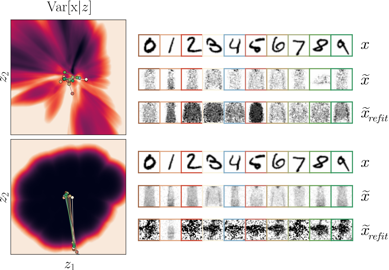

Image data. We evaluate the performance of our proposed dissipative V3AE (d-V3AE) against a fully Gaussian VAE on image data, coming from FashionMNIST, SVHN and CIFAR10. For both models, all parameter maps share the same underlying architecture, with the addition of either a softplus and/or a shifting last layer to ensure definition of both the variational and the generative distribution’s moments99 9 Full details are included in Sec. IV. of the supplements..
| FashionMNIST | SVHN | CIFAR | |||||
| VAE | |||||||
| d-V3AE | |||||||
| VAE | |||||||
| d-V3AE | |||||||
Tab. 2 compares model performance on two metrics, the log-likelihood and the RMSE between the original inputs x and reconstructed samples , where . Unlike most previous implementations, we focus on actual samples, and not the mean, of the generative distributions. This comparison emphasize the cooperation between the decoder’s mean and variance, allowing evaluation of the models’ uncertainty estimates. Our method both qualitatively (Fig. 9), and quantitatively improves on a Gaussian VAE’s sampling ability. The prior smoothens the uncertainty estimates, resulting in more realistic and less crisp samples. The log-likelihoods, evaluated at test time using truncation, i.e. , to account for the finite support of data, reveal that our model can achieve a better fit, if the prior is selected correctly. In SVHN and CIFAR10, the presence of color channels complicates the selection process and challenges our choice of a single homoscedastic prior for all pixels and channels. We note that the dissipative loss also applies to classic VAEs with Bernoulli-only decoders; see Sec. IV. of the supplements for details.
Applications of robust generative uncertainty. In Figs. 7 & 8, the colouring of the 2D latent space represent the aggregated decoder variance . It is clear that our method displays more regular uncertainty estimates, and provides the extrapolation guarantees we strove for. Beyond increased robustness and better generative power, this unlocks meaningful out-of-distribution detection, beating previous state-of-the-art (Havtorn et al. 2021)1010 10 Additional experiments are provided in Sec. IV..6. For Figs. 8 & 10, as argued in Mattei and Frellsen 2018b, we refit at test time the encoder of models trained on FashionMNIST on MNIST. The regularity and structure of the decoder variance rewards the encoder for learning to place representations of OOD data outside of the region of in-distribution latent encodings, resulting in a model that is aware of its own inability to reconstruct plausible data, as displayed by the row of d-V3AE.
4 Conclusion
We have introduced a novel loss, the dissipative loss, that leverages artificial out-of-distribution pseudo-inputs for learning robust uncertainty estimates. We demonstrate through a Bayesian approach that casts a prior distribution over the model’s variance a principled mechanism for controlling the extrapolation properties of neural networks governing the predictive uncertainty. Our results reflect the benefits of our principled and scalable approach, displaying better calibrated and more robust uncertainty estimates, while matching the predictive power of known baselines. Finally, and most interestingly, our approach can instill into probabilistic models a notion of their own ignorance, increasing their ability to know what they don’t know.
The main limitation of our approach is that it depends on an input density estimate. In our experience, even coarse-grained densities are sufficient to significantly improve upon current approaches. However, as one rarely have guaranteed good estimates of the input density, our method cannot be approached as a black-box. One exception seems to be the application to VAEs, where the aggregated posterior, in our experience, always provide a suitable density estimate.
References
- Xu et al. (2020) Keyulu Xu, Mozhi Zhang, Jingling Li, Simon S Du, Ken-ichi Kawarabayashi, and Stefanie Jegelka. How neural networks extrapolate: From feedforward to graph neural networks. arXiv preprint arXiv:2009.11848, 2020.
- Amodei et al. (2016) Dario Amodei, Chris Olah, Jacob Steinhardt, Paul Christiano, John Schulman, and Dan Mané. Concrete problems in ai safety. arXiv preprint arXiv:1606.06565, 2016.
- Hansen and Salamon (1990) Lars Kai Hansen and Peter Salamon. Neural network ensembles. IEEE transactions on pattern analysis and machine intelligence, 12(10):993–1001, 1990.
- Lakshminarayanan et al. (2017) Balaji Lakshminarayanan, Alexander Pritzel, and Charles Blundell. Simple and scalable predictive uncertainty estimation using deep ensembles. In Advances in neural information processing systems, pages 6402–6413, 2017.
- MacKay (1992) David JC MacKay. A practical bayesian framework for backpropagation networks. Neural computation, 4(3):448–472, 1992.
- Gal and Ghahramani (2016) Yarin Gal and Zoubin Ghahramani. Dropout as a bayesian approximation: Representing model uncertainty in deep learning. In international conference on machine learning, pages 1050–1059, 2016.
- Bishop (2006) Christopher M. Bishop. Pattern Recognition and Machine Learning. Springer, August 2006. ISBN 0387310738.
- Guo et al. (2017) Chuan Guo, Geoff Pleiss, Yu Sun, and Kilian Q Weinberger. On calibration of modern neural networks. arXiv preprint arXiv:1706.04599, 2017.
- Hendrycks and Gimpel (2016) Dan Hendrycks and Kevin Gimpel. A baseline for detecting misclassified and out-of-distribution examples in neural networks. arXiv preprint arXiv:1610.02136, 2016.
- Nalisnick et al. (2019) Eric Nalisnick, Akihiro Matsukawa, Yee Whye Teh, and Balaji Lakshminarayanan. Detecting out-of-distribution inputs to deep generative models using typicality. arXiv preprint arXiv:1906.02994, 2019.
- Nguyen et al. (2015) Anh Nguyen, Jason Yosinski, and Jeff Clune. Deep neural networks are easily fooled: High confidence predictions for unrecognizable images. In Proceedings of the IEEE conference on computer vision and pattern recognition, pages 427–436, 2015.
- Louizos and Welling (2017) Christos Louizos and Max Welling. Multiplicative normalizing flows for variational bayesian neural networks. arXiv preprint arXiv:1703.01961, 2017.
- Skafte et al. (2019) Nicki Skafte, Martin Jørgensen, and Søren Hauberg. Reliable training and estimation of variance networks. In Advances in Neural Information Processing Systems, pages 6326–6336, 2019.
- Lee et al. (2017) Kimin Lee, Honglak Lee, Kibok Lee, and Jinwoo Shin. Training confidence-calibrated classifiers for detecting out-of-distribution samples. arXiv preprint arXiv:1711.09325, 2017.
- Xu et al. (2021) Keyulu Xu, Mozhi Zhang, Jingling Li, Simon S. Du, Ken ichi Kawarabayashi, and Stefanie Jegelka. How neural networks extrapolate: From feedforward to graph neural networks, 2021.
- Nix and Weigend (1994) David A Nix and Andreas S Weigend. Estimating the mean and variance of the target probability distribution. In Proceedings of 1994 ieee international conference on neural networks (ICNN’94), volume 1, pages 55–60. IEEE, 1994.
- Hauberg (2019) Søren Hauberg. Only bayes should learn a manifold (on the estimation of differential geometric structure from data), 2019.
- Arvanitidis et al. (2017) Georgios Arvanitidis, Lars Kai Hansen, and Søren Hauberg. Latent space oddity: on the curvature of deep generative models. arXiv preprint arXiv:1710.11379, 2017.
- Kingma and Welling (2013) Diederik P Kingma and Max Welling. Auto-encoding variational bayes. arXiv preprint arXiv:1312.6114, 2013.
- Rezende et al. (2014) Danilo Jimenez Rezende, Shakir Mohamed, and Daan Wierstra. Stochastic backpropagation and approximate inference in deep generative models. arXiv preprint arXiv:1401.4082, 2014.
- Der Kiureghian and Ditlevsen (2009) Armen Der Kiureghian and Ove Ditlevsen. Aleatory or epistemic? does it matter? Structural safety, 31(2):105–112, 2009.
- Rasmussen and Williams (2005) Carl Edward Rasmussen and Christopher K. I. Williams. Gaussian Processes for Machine Learning (Adaptive Computation and Machine Learning). The MIT Press, 2005.
- Graves (2011) Alex Graves. Practical variational inference for neural networks. Advances in neural information processing systems, 24:2348–2356, 2011.
- Blundell et al. (2015) Charles Blundell, Julien Cornebise, Koray Kavukcuoglu, and Daan Wierstra. Weight uncertainty in neural networks. arXiv preprint arXiv:1505.05424, 2015.
- Hernández-Lobato and Adams (2015) José Miguel Hernández-Lobato and Ryan Adams. Probabilistic backpropagation for scalable learning of bayesian neural networks. In International Conference on Machine Learning, pages 1861–1869, 2015.
- Hasenclever et al. (2017) Leonard Hasenclever, Stefan Webb, Thibaut Lienart, Sebastian Vollmer, Balaji Lakshminarayanan, Charles Blundell, and Yee Whye Teh. Distributed bayesian learning with stochastic natural gradient expectation propagation and the posterior server. The Journal of Machine Learning Research, 18(1):3744–3780, 2017.
- Welling and Teh (2011) Max Welling and Yee W Teh. Bayesian learning via stochastic gradient langevin dynamics. In Proceedings of the 28th international conference on machine learning (ICML-11), pages 681–688, 2011.
- Springenberg et al. (2016) Jost Tobias Springenberg, Aaron Klein, Stefan Falkner, and Frank Hutter. Bayesian optimization with robust bayesian neural networks. Advances in neural information processing systems, 29:4134–4142, 2016.
- Breiman (1996) Leo Breiman. Bagging predictors. Machine learning, 24(2):123–140, 1996.
- Thagaard et al. (2020) Jeppe Thagaard, Søren Hauberg, Bert van der Vegt, Thomas Ebstrup, Johan D. Hansen, and Anders B. Dahl. Can you trust predictive uncertainty under real dataset shifts in digital pathology? In Medical Image Computing and Computer-Assisted Intervention (MICCAI), Lima, Peru, October 2020.
- Ovadia et al. (2019) Yaniv Ovadia, Emily Fertig, Jie Ren, Zachary Nado, David Sculley, Sebastian Nowozin, Joshua Dillon, Balaji Lakshminarayanan, and Jasper Snoek. Can you trust your model’s uncertainty? evaluating predictive uncertainty under dataset shift. In Advances in Neural Information Processing Systems, pages 13991–14002, 2019.
- Breiman (2001) Leo Breiman. Random forests. Machine learning, 45(1):5–32, 2001.
- Srivastava et al. (2014) Nitish Srivastava, Geoffrey Hinton, Alex Krizhevsky, Ilya Sutskever, and Ruslan Salakhutdinov. Dropout: a simple way to prevent neural networks from overfitting. The journal of machine learning research, 15(1):1929–1958, 2014.
- Liang et al. (2017) Shiyu Liang, Yixuan Li, and Rayadurgam Srikant. Enhancing the reliability of out-of-distribution image detection in neural networks. arXiv preprint arXiv:1706.02690, 2017.
- Goodfellow et al. (2014a) Ian J Goodfellow, Jonathon Shlens, and Christian Szegedy. Explaining and harnessing adversarial examples. arXiv preprint arXiv:1412.6572, 2014a.
- Hendrycks et al. (2018) Dan Hendrycks, Mantas Mazeika, and Thomas Dietterich. Deep anomaly detection with outlier exposure. arXiv preprint arXiv:1812.04606, 2018.
- Goodfellow et al. (2014b) Ian Goodfellow, Jean Pouget-Abadie, Mehdi Mirza, Bing Xu, David Warde-Farley, Sherjil Ozair, Aaron Courville, and Yoshua Bengio. Generative adversarial nets. Advances in neural information processing systems, 27:2672–2680, 2014b.
- Dai et al. (2017) Zihang Dai, Zhilin Yang, Fan Yang, William W Cohen, and Russ R Salakhutdinov. Good semi-supervised learning that requires a bad gan. In Advances in neural information processing systems, pages 6510–6520, 2017.
- Jain et al. (2020) Siddhartha Jain, Ge Liu, Jonas Mueller, and David Gifford. Maximizing overall diversity for improved uncertainty estimates in deep ensembles. In Proceedings of the AAAI Conference on Artificial Intelligence, volume 34, pages 4264–4271, 2020.
- Hafner et al. (2018) Danijar Hafner, Dustin Tran, Timothy Lillicrap, Alex Irpan, and James Davidson. Reliable uncertainty estimates in deep neural networks using noise contrastive priors. 2018.
- Malinin and Gales (2018) Andrey Malinin and Mark Gales. Predictive uncertainty estimation via prior networks. arXiv preprint arXiv:1802.10501, 2018.
- Ioffe and Szegedy (2015) Sergey Ioffe and Christian Szegedy. Batch normalization: Accelerating deep network training by reducing internal covariate shift. In International conference on machine learning, pages 448–456. PMLR, 2015.
- Mattei and Frellsen (2018a) Pierre-Alexandre Mattei and Jes Frellsen. Leveraging the exact likelihood of deep latent variable models. In Advances in Neural Information Processing Systems, pages 3855–3866, 2018a.
- Gelman et al. (2013) Andrew Gelman, John B Carlin, Hal S Stern, David B Dunson, Aki Vehtari, and Donald B Rubin. Bayesian data analysis. CRC press, 2013.
- Jørgensen (2020) Martin Jørgensen. Stochastic Representations with Gaussian Processes and Geometry. PhD thesis, Technical University of Denmark, 2020.
- Stirn and Knowles (2020) Andrew Stirn and David A Knowles. Variational variance: Simple and reliable predictive variance parameterization. arXiv preprint arXiv:2006.04910, 2020.
- Lee and Wang (2003) Elisa T Lee and John Wang. Statistical methods for survival data analysis, volume 476. John Wiley & Sons, 2003.
- Shrivastava et al. (2017) Ashish Shrivastava, Tomas Pfister, Oncel Tuzel, Joshua Susskind, Wenda Wang, and Russell Webb. Learning from simulated and unsupervised images through adversarial training. In Proceedings of the IEEE conference on computer vision and pattern recognition, pages 2107–2116, 2017.
- Dawid (1982) A Philip Dawid. The well-calibrated bayesian. Journal of the American Statistical Association, 77(379):605–610, 1982.
- Blei et al. (2017) David M Blei, Alp Kucukelbir, and Jon D McAuliffe. Variational inference: A review for statisticians. Journal of the American statistical Association, 112(518):859–877, 2017.
- Foong et al. (2019) Andrew YK Foong, Yingzhen Li, José Miguel Hernández-Lobato, and Richard E Turner. ’in-between’uncertainty in bayesian neural networks. arXiv preprint arXiv:1906.11537, 2019.
- Havtorn et al. (2021) Jakob D. Havtorn, Jes Frellsen, Søren Hauberg, and Lars Maaløe. Hierarchical vaes know what they don’t know, 2021.
- Mattei and Frellsen (2018b) P.-A Mattei and J Frellsen. Refit your encoder when new data comes by. In 3rd NeurIPS workshop on Bayesian Deep Learning, 2018b.
- Johnson et al. (1994) Norman L Johnson, Samuel Kotz, and Narayanaswamy Balakrishnan. Continuous univariate distributions, volume 1, 2nd Edition. John wiley & sons, 1994.
- Bauckhage (2014) Christian Bauckhage. Computing the kullback-leibler divergence between two generalized gamma distributions. arXiv preprint arXiv:1401.6853, 2014.
- Kingma and Ba (2014) Diederik P Kingma and Jimmy Ba. Adam: A method for stochastic optimization. arXiv preprint arXiv:1412.6980, 2014.
I. Student-t likelihood
I..1 Marginal distribution of a Gaussian likelihood with a Gamma precision
In the case of a Gaussian likelihood with a latent Gamma distributed precision, the marginal distribution follows:
| (7) | ||||
The moments of the marginal distribution are, assuming ,
| (8) |
I..2 Decomposition of a Student-t’s uncertainty
The variance of a non standard Student-t distribution with degrees of freedom and scaled by can be decomposed as . The number of degrees of freedom scales with the number of observations that the distribution arises from. When the number of observations grows towards , i.e towards perfect information, the term converges towards 1, motivating its casting into an epistemic factor. The natural consequence is that , which accounts for the rest of the model’s uncertainty, scales as the aleatoric uncertainty. For more details see Jørgensen 2020.
II. Pseudo-inputs generator
II..1 On boundary samples
| method | CCPP | Wine-white |
| No OOD (VV) | 0.655 | 1.719 |
| Boundary OOD (d-VV) | 0.019 | 0.072 |
| Far OOD (d-VV) | 0.023 | 0.941 |
Tab. 3 provides supporting evidence regarding the benefits of placing pseudo-inputs close to the training distribution. It compares the mean measured OOD KL divergence over 5 trials for two different UCI regression datasets. The boundary OOD pseudo-inputs were generated using the proposed density-based generation procedure. The far OOD pseudo-inputs were generated by adding large Gaussian noise ( for standardised inputs) to training points. Boundary OOD pseudo-inputs result in a lower OOD prior KL divergence, meaning that the regularisation is indeed enforced in most of the OOD support.
II..2 Sensitivity to hyperparameters
The pseudo-input generator hyperparameters were chosen through a coarse grid search on a sub selection of experiments from the UCI benchmarks, and applied to the rest of the experiments. In practice we observed that Alg. 1 is relatively insensitive to hyperparameters. For example the Tab. 5 below describes the evolution of the ELBO and the log-likelihood as a function of the number of steps on the Carbon UCI dataset. The ELBO and LLK here have opposite evolutions based on the number of steps - hence our practical choice of a “middle ground” with n = 5. Tab. 5 evaluates similarly the influence of the threshold parameter. The results are naturally varying depending on the dataset chosen, as different overall input densities will more or less allow the gradient descent iterations to modify the original distribution of noisy pseudo-inputs. We regard this as a strength of our proposed method, if the distribution of pseudo-inputs can be improved and better separated from the training input distribution, it will leverage this possibility, but if it’s not the case, pseudo inputs will not vary from their original position, generated as if they were inputs perturbed by Gaussian noise.
II..3 Influence of the pseudo-input generator
We originally envisioned to generate pseudo-inputs using the same Gaussian perturbation technique as independently proposed in Hafner et al. 2018, where . We nevertheless quickly come to realise that this does not actually produce pseudo-inputs that are guaranteed to be out-of-distribution, and eventually result in over-regularisation. Tab. 6 compares the mean ELBO over 5 trials of our proposal with selected parameters for the gradient descent (dVV), with our proposal without any gradient descent (dVV - 0 steps) and our method with pseudo-inputs generated as Gaussian noise (dVV - Gaussian noise, as is done in Hafner et al. 2018) on the UCI benchmark. We observe that, as expected, better pseudo-inputs placement results in our method performing better on a larger selection of experiments (8/12).
| method | Boston | Carbon | CCPP | Concrete | Energy | Kin8nm | Naval | Protein | Superconduct | Wine-red | Wine-white | Yacht |
| d-VV | -0.614 | 1.191 | -0.141 | -0.443 | 0.665 | -0.247 | 0.522 | -1.319 | -0.543 | -1.997 | -1.822 | -17.599 |
| d-VV | -0.658 | 1.229 | -0.131 | -0.433 | 0.656 | -0.255 | 0.496 | -1.317 | -0.558 | -2.192 | -2.03 | -21.802 |
| (0 steps) | ||||||||||||
| d-VV | -0.819 | -0.473 | -0.569 | -0.645 | -0.515 | -0.591 | -0.537 | -1.236 | -0.724 | -1.747 | -1.554 | -0.507 |
| (Gaussian noise) |
II..4 Number of pseudo-inputs
In our implementation, to stabilise training, we use the expected value over each dataset (in or out-of-distribution) by dividing each term by the number of data points used to compute them. This results in a very limited sensibility of our practical implementation in the number of pseudo-inputs used.
III. Regression experiments
III..1 Variational Variance’s ELBO Closed Form
For a Gaussian likelihood and a Gamma posterior, both terms of the ELBO have a closed form solution. Firstly the expected log-likelihood verifies:
| (9) | ||||
The variational posterior being Gamma distributed, its expected value is defined as . The logarithmic expectation of a Gamma distribution can be derived to yield (Johnson et al. 1994, 337–349) where is the digamma function. The closed-form expression of the expected likelihood is therefore:
| (10) |
Secondly, the KL-divergence between the posterior and the prior can be derived from Equation (28) in Bauckhage 2014. With Bauckhage’s notation, setting , to correspond to standard Gamma distributions, shape parameters and , and scale parameters and the KL-divergence can be expressed as
| (11) | ||||
III..2 True posterior and heteroscedasticity
The true posterior for variational variance in a regression context can be written . As first demonstrated in Sec. 8.2 of Stirn and Knowles 2020, it factorizes as:
| (12) | ||||
| (13) | ||||
| (14) | ||||
| (15) |
As a result, the true posterior both depends on the inputs and targets . It means that a single input, could theoretically imply different latent precisions for different targets , thus violating the x-surjectivity of the heteroscedastic definition.
III..3 Model architecture
We adopted a unified network architecture for the regression case. All neural-network parameter maps share the same underlying architecture, a single hidden layer with 50 hidden units using exponential linear unit (ELU) activation functions. A final softplus layer is applied on the last layer of the , and parameter maps. The parameter map is further shifted by +1 to ensure the definition of the marginal distribution’s variance. Regression models are trained with the Adam (Kingma and Ba 2014) optimiser, and both the inputs and targets are standardised prior to training and testing.
III..4 Pseudo-input generator
Tab. 7 presents the parameters used by the PIG in a regression setting. We remind that these parameters are parameters of a gradient descent, with learning rate .
| K | max_iterations | tolerance | |
| N | 5 | 0.005 | 4-1 |
For our experiments, we approximated the input density with a Bayesian Gaussian mixture model1111 11 https://scikit-learn.org/stable/modules/generated/sklearn.mixture.BayesianGaussianMixture.html with diagonal covariance matrices, and initialised with as many components as there are inputs in a batch.
III..5 UCI experiments
| Name | Dimensions () | Link (https://archive.ics.uci.edu/ml/*) |
| Boston | (505,13,1) | machine-learning-databases/housing/ |
| Carbon | (10721,5,3) | datasets/Carbon+Nanotubes |
| Concrete | (1030,8,1) | datasets/Concrete+Compressive+Strength |
| Energy | (768,8,2) | datasets/Energy+efficiency |
| Kin8nm | (8192,8,1) | https://www.openml.org/d/189 |
| Naval | (11934,16,2) | datasets/Condition+Based+Maintenance+of+Naval+Propulsion+Plants |
| Power plant (CCPP) | (9568,4,1) | datasets/Combined+Cycle+Power+Plant |
| Protein | (45630, 9, 1) | datasets/Physicochemical+Properties+of+Protein+Tertiary+Structure |
| Superconductivity | (21263,81,1) | datasets/Superconductivty+Data |
| Wine-red | (1599,11,1) | datasets/Wine+Quality |
| Wine-white | (4898,11,1) | datasets/Wine+Quality |
| Yacht | (308,6,1) | datasets/Yacht+Hydrodynamics |
The UCI experiments (https://archive.ics.uci.edu/ml/datasets.php) consist of the datasets presented in Tab. 8.
The results, for the different metrics, as presented in Tab. 11 to 16, were computed as the mean the standard deviation over 5 trials with standardised inputs and targets. Due to a technical error, we were forced to re-run the experiments for d-VV and VV (no PIG) right before the submission deadline, and reduced the number of trials to 3 for these methods.
A method is deemed to perform best for a given metric when the mean of the evaluated metric is the best across methods. For determining statistical draws we ran for each method a two-sided test for verifying whether the mean of the evaluated metric is significantly different to the mean of the best method . To do so, we test for , under a Gaussian distribution with standard deviation at a 0.05 level.
III..6 Aggregate benchmark data
| UCI benchmarks (shifts not included) | d-VV | VV | VV (no prior) | Mean variance network | Skafte et al | Deep ensembles | Monte Carlo dropout | Noise contrastive priors | Bayes by backprop | |||||||||
| 11 / | 8 | 1 / | 1 | 0 / | 0 | n / | a | n / | a | n / | a | n / | a | n / | a | n / | a | |
| 1 / | 1 | 3 / | 6 | 0 / | 0 | 0 / | 0 | 1 / | 2 | 0 / | 0 | 0 / | 0 | 0 / | 0 | 7 / | 6 | |
| 2 / | 2 | 1 / | 4 | 1 / | 3 | 0 / | 0 | 0 / | 0 | 4 / | 10 | 0 / | 0 | 0 / | 0 | 4 / | 0 | |
| 2 / | 4 | 3 / | 4 | 1 / | 2 | 0 / | 0 | n / | a | 1 / | 3 | 1 / | 2 | 0 / | 0 | 4 / | 4 | |
| 2 / | 2 | 3 / | 3 | 2 / | 1 | n / | a | n / | a | n / | a | n / | a | 0 / | 0 | 5 / | 3 | |
| 12 / | 7 | 0 / | 0 | 0 / | 0 | n / | a | n / | a | n / | a | n / | a | n / | a | n / | a | |
| UCI benchmarks (only shifts) | d-VV | VV | VV (no prior) | Mean variance network | Skafte et al | Deep ensembles | Monte Carlo dropout | Noise contrastive priors | Bayes by backprop | |||||||||
| 10 / | 10 | 2 / | 2 | 0 / | 0 | n / | a | n / | a | n / | a | n / | a | n / | a | n / | a | |
| 1 / | 6 | 2 / | 3 | 0 / | 0 | 0 / | 0 | 3 / | 7 | 0 / | 0 | 0 / | 0 | 2 / | 8 | 4 / | 2 | |
| 0 / | 0 | 0 / | 0 | 1 / | 2 | 1 / | 5 | 2 / | 3 | 1 / | 2 | 3 / | 16 | 0 / | 0 | 4 / | 0 | |
| 0 / | 0 | 2 / | 5 | 1 / | 2 | 0 / | 0 | n / | a | 1 / | 2 | 4 / | 15 | 0 / | 0 | 4 / | 3 | |
| 1 / | 2 | 2 / | 4 | 2 / | 1 | n / | a | n / | a | n / | a | n / | a | 1 / | 2 | 6 / | 4 | |
| 11 / | 7 | 1 / | 0 | 0 / | 0 | n / | a | n / | a | n / | a | n / | a | n / | a | n / | a | |
III..7 Benchmark raw data
| UCI benchmarks | d-VV | VV | VV (no prior) | Mean variance network | Skafte et al | Deep ensembles | Monte Carlo dropout | Noise contrastive priors | Bayes by backprop | ||||||||||
| Not shifted | uci_boston | -0.61 | 0.33 | -0.72 | 0.38 | -64.28 | 29.34 | nan | nan | nan | nan | nan | nan | nan | nan | nan | nan | nan | nan |
| uci_carbon | 1.19 | 0.11 | 1.17 | 0.12 | -3913.5 | 580.03 | nan | nan | nan | nan | nan | nan | nan | nan | nan | nan | nan | nan | |
| uci_ccpp | -0.14 | 0.01 | -0.16 | 0.04 | -10.9 | 1.06 | nan | nan | nan | nan | nan | nan | nan | nan | nan | nan | nan | nan | |
| uci_concrete | -0.44 | 0.13 | -0.46 | 0.08 | -44.06 | 14.23 | nan | nan | nan | nan | nan | nan | nan | nan | nan | nan | nan | nan | |
| uci_energy | 0.67 | 0.03 | 0.65 | 0.03 | -118.78 | 81.29 | nan | nan | nan | nan | nan | nan | nan | nan | nan | nan | nan | nan | |
| uci_kin8nm | -0.25 | 0.02 | -0.28 | 0.04 | -16.76 | 1.53 | nan | nan | nan | nan | nan | nan | nan | nan | nan | nan | nan | nan | |
| uci_naval | 0.52 | 0.16 | 0.12 | 0.4 | -9.57 | 4.57 | nan | nan | nan | nan | nan | nan | nan | nan | nan | nan | nan | nan | |
| uci_protein | -1.32 | 0.01 | -1.34 | 0.01 | -14.31 | 2.59 | nan | nan | nan | nan | nan | nan | nan | nan | nan | nan | nan | nan | |
| uci_superconduct | -0.54 | 0.03 | -0.56 | 0.01 | -269.08 | 58.88 | nan | nan | nan | nan | nan | nan | nan | nan | nan | nan | nan | nan | |
| uci_wine_red | -2.0 | 0.08 | -2.36 | 0.19 | -37.86 | 31.48 | nan | nan | nan | nan | nan | nan | nan | nan | nan | nan | nan | nan | |
| uci_wine_white | -1.82 | 0.06 | -2.01 | 0.1 | -869.26 | 1718.81 | nan | nan | nan | nan | nan | nan | nan | nan | nan | nan | nan | nan | |
| uci_yacht | -17.6 | 0.43 | 1.04 | 0.1 | -551.12 | 1060.39 | nan | nan | nan | nan | nan | nan | nan | nan | nan | nan | nan | nan | |
| Shifted | uci_boston | -1.28 | 0.32 | -1.47 | 0.28 | -110.63 | 110.55 | nan | nan | nan | nan | nan | nan | nan | nan | nan | nan | nan | nan |
| uci_carbon | 1.16 | 0.02 | 1.11 | 0.03 | -3991.86 | 679.64 | nan | nan | nan | nan | nan | nan | nan | nan | nan | nan | nan | nan | |
| uci_ccpp | -0.25 | 0.08 | -0.33 | 0.14 | -8.36 | 1.65 | nan | nan | nan | nan | nan | nan | nan | nan | nan | nan | nan | nan | |
| uci_concrete | -1.29 | 0.27 | -1.51 | 0.38 | -75.74 | 59.7 | nan | nan | nan | nan | nan | nan | nan | nan | nan | nan | nan | nan | |
| uci_energy | -0.69 | 1.1 | -0.56 | 0.9 | -891.92 | 1570.09 | nan | nan | nan | nan | nan | nan | nan | nan | nan | nan | nan | nan | |
| uci_kin8nm | -0.33 | 0.03 | -0.38 | 0.04 | -23.9 | 1.92 | nan | nan | nan | nan | nan | nan | nan | nan | nan | nan | nan | nan | |
| uci_naval | -4.73 | 4.61 | -5.31 | 6.58 | -26.02 | 48.06 | nan | nan | nan | nan | nan | nan | nan | nan | nan | nan | nan | nan | |
| uci_protein | -1.56 | 0.11 | -1.64 | 0.16 | -9.34 | 6.68 | nan | nan | nan | nan | nan | nan | nan | nan | nan | nan | nan | nan | |
| uci_superconduct | -1.43 | 0.32 | -1.52 | 0.34 | -224.0 | 111.57 | nan | nan | nan | nan | nan | nan | nan | nan | nan | nan | nan | nan | |
| uci_wine_red | -2.84 | 0.21 | -3.45 | 0.35 | -47.78 | 56.02 | nan | nan | nan | nan | nan | nan | nan | nan | nan | nan | nan | nan | |
| uci_wine_white | -2.04 | 0.11 | -2.53 | 0.29 | -346.83 | 434.27 | nan | nan | nan | nan | nan | nan | nan | nan | nan | nan | nan | nan | |
| uci_yacht | -7.59 | 2.58 | 0.35 | 0.19 | -194.42 | 149.45 | nan | nan | nan | nan | nan | nan | nan | nan | nan | nan | nan | nan | |
| UCI benchmarks | d-VV | VV | VV (no prior) | Mean variance network | Skafte et al | Deep ensembles | Monte Carlo dropout | Noise contrastive priors | Bayes by backprop | ||||||||||
| Not shifted | uci_boston | -0.43 | 0.35 | -0.42 | 0.39 | -3.34 | 1.39 | -0.76 | 0.07 | -0.18 | 0.19 | -0.68 | 0.04 | -0.81 | 0.51 | -1.39 | 0.33 | -248.43 | 163.55 |
| uci_carbon | 1.45 | 0.13 | 1.45 | 0.11 | 0.98 | 3.08 | -3.78 | 0.05 | 1.13 | 0.51 | -3.71 | 0.04 | 0.29 | 1.08 | nan | nan | nan | nan | |
| uci_ccpp | -0.07 | 0.01 | -0.03 | 0.03 | 0.05 | 0.06 | -0.58 | 0.14 | -0.18 | 0.12 | -0.61 | 0.05 | -3.36 | 0.56 | 0.21 | 0.04 | 4.06 | 0.69 | |
| uci_concrete | -0.29 | 0.15 | -0.25 | 0.1 | -0.83 | 0.5 | -0.68 | 0.09 | -0.4 | 0.15 | -0.65 | 0.04 | -0.9 | 0.33 | 0.38 | 0.04 | 3.84 | 0.66 | |
| uci_energy | 0.87 | 0.04 | 0.89 | 0.03 | 0.47 | 0.2 | -1.22 | 0.11 | 0.28 | 0.37 | -1.17 | 0.04 | 0.36 | 0.26 | nan | nan | nan | nan | |
| uci_kin8nm | -0.17 | 0.02 | -0.15 | 0.04 | -0.36 | 0.07 | -0.61 | 0.06 | -0.61 | 0.12 | -0.65 | 0.03 | -0.63 | 0.05 | -0.68 | 0.08 | -0.16 | 0.03 | |
| uci_naval | 0.71 | 0.19 | 0.52 | 0.2 | -0.13 | 0.32 | -2.26 | 0.08 | -2.67 | 0.22 | -2.26 | 0.06 | -0.2 | 0.74 | nan | nan | nan | nan | |
| uci_protein | -1.16 | 0.01 | -1.12 | 0.01 | -1.42 | 0.38 | -1.13 | 0.05 | -1.54 | 0.74 | -1.05 | 0.01 | -7.41 | 0.27 | -1.02 | 0.01 | -0.96 | 0.02 | |
| uci_superconduct | -0.38 | 0.02 | -0.35 | 0.02 | -1.73 | 1.71 | -0.66 | 0.04 | -0.96 | 0.18 | -0.68 | 0.03 | -1.72 | 0.25 | -0.2 | 0.19 | -0.04 | 0.06 | |
| uci_wine_red | -1.91 | 0.07 | -2.13 | 0.21 | -7.77 | 6.39 | -2560.95 | 5395.69 | -1.15 | 0.04 | -1.24 | 0.08 | -4.24 | 0.91 | 0.16 | 0.04 | 3.76 | 0.39 | |
| uci_wine_white | -1.72 | 0.06 | -1.75 | 0.1 | -305.7 | 549.73 | -27.69 | 48.8 | -1.4 | 0.58 | -1.16 | 0.08 | -5.86 | 1.08 | 0.29 | 0.06 | 3.76 | 0.82 | |
| uci_yacht | 0.9 | 0.02 | 1.33 | 0.11 | 0.63 | 0.59 | -0.59 | 0.11 | 0.4 | 0.14 | -0.58 | 0.04 | 0.33 | 0.69 | 0.63 | 0.1 | 1.57 | 0.6 | |
| Shifted | uci_boston | -1.09 | 0.32 | -1.16 | 0.27 | -10.33 | 10.87 | -0.84 | 0.09 | -0.16 | 0.09 | -0.79 | 0.07 | -2.52 | 1.34 | -3.83 | 1.82 | -428.29 | 194.72 |
| uci_carbon | 1.34 | 0.06 | 1.4 | 0.02 | -0.6 | 2.9 | -3.87 | 0.34 | 1.12 | 0.25 | -3.71 | 0.12 | 0.55 | 0.1 | nan | nan | nan | nan | |
| uci_ccpp | -0.18 | 0.09 | -0.2 | 0.14 | -0.1 | 0.08 | -0.54 | 0.04 | -0.16 | 0.02 | -0.65 | 0.02 | -4.31 | 0.43 | 0.2 | 0.07 | 3.76 | 0.75 | |
| uci_concrete | -1.11 | 0.27 | -1.23 | 0.36 | -10.81 | 15.27 | -0.77 | 0.1 | -0.38 | 0.06 | -0.78 | 0.04 | -2.38 | 0.52 | 0.29 | 0.05 | 4.17 | 0.36 | |
| uci_energy | -0.47 | 1.15 | -0.2 | 0.76 | -96.95 | 259.19 | -1.42 | 0.26 | 0.2 | 0.25 | -1.36 | 0.23 | -1.13 | 2.52 | nan | nan | nan | nan | |
| uci_kin8nm | -0.26 | 0.04 | -0.22 | 0.04 | -0.88 | 0.14 | -0.64 | 0.09 | -0.59 | 0.04 | -0.65 | 0.05 | -0.86 | 0.21 | -0.68 | 0.09 | -0.26 | 0.1 | |
| uci_naval | -4.55 | 4.62 | -5.01 | 6.53 | -14.78 | 18.92 | -3.59 | 0.89 | -2.76 | 0.15 | -3.62 | 0.89 | -22.29 | 12.05 | nan | nan | nan | nan | |
| uci_protein | -1.44 | 0.12 | -1.42 | 0.15 | -2.26 | 1.3 | -1.33 | 0.09 | -1.51 | 0.46 | -1.21 | 0.07 | -9.94 | 1.27 | -1.16 | 0.06 | -1.21 | 0.09 | |
| uci_superconduct | -1.28 | 0.32 | -1.28 | 0.33 | -8.32 | 11.59 | -0.98 | 0.11 | -1.06 | 0.16 | -0.9 | 0.06 | -5.9 | 1.74 | -0.72 | 0.28 | -2.87 | 5.54 | |
| uci_wine_red | -2.7 | 0.2 | -3.1 | 0.32 | -12.13 | 13.11 | -229.56 | 749.24 | -1.14 | 0.02 | -1.57 | 0.26 | -4.42 | 0.5 | 0.13 | 0.1 | 3.84 | 0.44 | |
| uci_wine_white | -1.97 | 0.12 | -2.24 | 0.27 | -183.07 | 323.25 | -1.75 | 0.23 | -1.3 | 0.13 | -1.29 | 0.04 | -5.65 | 0.49 | 0.3 | 0.04 | 3.61 | 0.88 | |
| uci_yacht | 0.71 | 0.76 | 0.65 | 0.19 | 0.51 | 0.55 | -0.53 | 0.05 | 0.43 | 0.07 | -0.58 | 0.05 | 0.37 | 0.35 | 0.41 | 0.2 | -11.62 | 25.18 | |
| UCI benchmarks | d-VV | VV | VV (no prior) | Mean variance network | Skafte et al | Deep ensembles | Monte Carlo dropout | Noise contrastive priors | Bayes by backprop | ||||||||||
| Not shifted | uci_boston | 0.33 | 0.09 | 0.33 | 0.08 | 0.38 | 0.09 | 0.35 | 0.06 | 0.3 | 0.07 | 0.29 | 0.05 | 0.33 | 0.05 | 0.47 | 0.06 | 0.5 | 0.04 |
| uci_carbon | 0.03 | 0.02 | 0.03 | 0.02 | 0.03 | 0.02 | 0.75 | 0.01 | 0.09 | 0.08 | 0.75 | 0.01 | 0.08 | 0.0 | nan | nan | nan | nan | |
| uci_ccpp | 0.23 | 0.01 | 0.23 | 0.01 | 0.23 | 0.01 | 0.23 | 0.01 | 0.27 | 0.03 | 0.23 | 0.01 | 0.24 | 0.01 | 0.07 | 0.03 | 0.0 | 0.0 | |
| uci_concrete | 0.29 | 0.04 | 0.29 | 0.04 | 0.33 | 0.04 | 0.29 | 0.01 | 0.35 | 0.07 | 0.27 | 0.01 | 0.28 | 0.02 | 0.08 | 0.02 | 0.0 | 0.0 | |
| uci_energy | 0.08 | 0.01 | 0.08 | 0.01 | 0.3 | 0.03 | 0.13 | 0.01 | 0.22 | 0.08 | 0.13 | 0.01 | 0.13 | 0.02 | nan | nan | nan | nan | |
| uci_kin8nm | 0.26 | 0.01 | 0.26 | 0.01 | 0.28 | 0.01 | 0.27 | 0.01 | 0.44 | 0.07 | 0.26 | 0.01 | 0.33 | 0.01 | 0.4 | 0.07 | 0.29 | 0.0 | |
| uci_naval | 0.09 | 0.06 | 0.1 | 0.03 | 0.33 | 0.07 | 0.72 | 0.01 | 0.86 | 0.09 | 0.72 | 0.01 | 0.2 | 0.07 | nan | nan | nan | nan | |
| uci_protein | 0.71 | 0.01 | 0.71 | 0.0 | 0.75 | 0.01 | 0.71 | 0.01 | 1.12 | 0.73 | 0.69 | 0.01 | 0.7 | 0.01 | 0.76 | 0.02 | 0.73 | 0.01 | |
| uci_superconduct | 0.35 | 0.01 | 0.35 | 0.01 | 0.4 | 0.02 | 0.35 | 0.01 | 0.67 | 0.22 | 0.32 | 0.01 | 0.33 | 0.01 | 0.44 | 0.03 | 0.41 | 0.01 | |
| uci_wine_red | 0.89 | 0.01 | 0.9 | 0.04 | 0.77 | 0.07 | 1.13 | 0.15 | 0.76 | 0.02 | 0.84 | 0.06 | 0.77 | 0.05 | 0.1 | 0.04 | 0.01 | 0.0 | |
| uci_wine_white | 0.9 | 0.03 | 0.88 | 0.02 | 0.82 | 0.06 | 0.85 | 0.05 | 0.93 | 0.39 | 0.77 | 0.06 | 0.79 | 0.05 | 0.08 | 0.04 | 0.01 | 0.0 | |
| uci_yacht | 0.05 | 0.02 | 0.04 | 0.02 | 0.82 | 0.12 | 0.05 | 0.01 | 0.09 | 0.06 | 0.05 | 0.01 | 0.11 | 0.04 | 0.09 | 0.02 | 0.16 | 0.03 | |
| Shifted | uci_boston | 0.52 | 0.08 | 0.52 | 0.08 | 0.43 | 0.1 | 0.48 | 0.07 | 0.3 | 0.04 | 0.44 | 0.08 | 0.41 | 0.06 | 0.5 | 0.07 | 0.46 | 0.06 |
| uci_carbon | 0.03 | 0.0 | 0.03 | 0.0 | 0.03 | 0.0 | 0.72 | 0.05 | 0.1 | 0.03 | 0.72 | 0.05 | 0.08 | 0.0 | nan | nan | nan | nan | |
| uci_ccpp | 0.26 | 0.02 | 0.26 | 0.03 | 0.25 | 0.01 | 0.25 | 0.01 | 0.26 | 0.01 | 0.25 | 0.01 | 0.25 | 0.01 | 0.07 | 0.04 | 0.01 | 0.0 | |
| uci_concrete | 0.54 | 0.07 | 0.54 | 0.07 | 0.44 | 0.05 | 0.48 | 0.05 | 0.35 | 0.03 | 0.43 | 0.05 | 0.4 | 0.04 | 0.09 | 0.03 | 0.0 | 0.0 | |
| uci_energy | 0.26 | 0.23 | 0.26 | 0.22 | 0.39 | 0.14 | 0.28 | 0.19 | 0.23 | 0.05 | 0.22 | 0.11 | 0.22 | 0.11 | nan | nan | nan | nan | |
| uci_kin8nm | 0.28 | 0.01 | 0.28 | 0.01 | 0.29 | 0.01 | 0.29 | 0.01 | 0.43 | 0.02 | 0.27 | 0.01 | 0.36 | 0.02 | 0.37 | 0.08 | 0.31 | 0.02 | |
| uci_naval | 1.37 | 0.96 | 1.35 | 0.95 | 1.61 | 0.71 | 0.89 | 0.11 | 0.9 | 0.06 | 0.89 | 0.1 | 1.32 | 0.59 | nan | nan | nan | nan | |
| uci_protein | 0.83 | 0.04 | 0.83 | 0.05 | 0.84 | 0.04 | 0.84 | 0.05 | 1.02 | 0.22 | 0.8 | 0.05 | 0.8 | 0.03 | 0.82 | 0.03 | 0.81 | 0.03 | |
| uci_superconduct | 0.59 | 0.07 | 0.59 | 0.06 | 0.52 | 0.06 | 0.6 | 0.06 | 0.6 | 0.08 | 0.52 | 0.05 | 0.51 | 0.05 | 0.54 | 0.06 | 0.53 | 0.05 | |
| uci_wine_red | 1.13 | 0.05 | 1.14 | 0.05 | 0.79 | 0.03 | 1.62 | 0.21 | 0.76 | 0.01 | 1.03 | 0.11 | 0.84 | 0.03 | 0.11 | 0.05 | 0.01 | 0.0 | |
| uci_wine_white | 0.96 | 0.04 | 0.96 | 0.04 | 0.87 | 0.03 | 1.03 | 0.07 | 0.84 | 0.05 | 0.86 | 0.03 | 0.86 | 0.04 | 0.06 | 0.02 | 0.01 | 0.0 | |
| uci_yacht | 0.16 | 0.08 | 0.1 | 0.04 | 0.74 | 0.22 | 0.09 | 0.03 | 0.07 | 0.02 | 0.07 | 0.02 | 0.13 | 0.04 | 0.11 | 0.02 | 0.18 | 0.06 | |
| UCI benchmarks | d-VV | VV | VV (no prior) | Mean variance network | Skafte et al | Deep ensembles | Monte Carlo dropout | Noise contrastive priors | Bayes by backprop | ||||||||||
| Not shifted | uci_boston | 0.25 | 0.11 | 0.37 | 0.26 | 1.000000e+11 | 3.162278e+11 | 0.61 | 0.14 | nan | nan | 0.53 | 0.06 | 0.29 | 0.17 | 36.0 | 4.18 | 0.77 | 0.31 |
| uci_carbon | 0.05 | 0.04 | 0.05 | 0.04 | 0.03 | 0.03 | 1.68 | 0.06 | nan | nan | 1.6 | 0.03 | 0.09 | 0.01 | nan | nan | nan | nan | |
| uci_ccpp | 0.15 | 0.01 | 0.15 | 0.01 | 0.24 | 0.3 | 0.5 | 0.18 | nan | nan | 0.47 | 0.04 | 0.14 | 0.04 | 0.13 | 0.01 | 0.0 | 0.0 | |
| uci_concrete | 0.24 | 0.15 | 0.22 | 0.13 | 1.32 | 3.53 | 0.55 | 0.15 | nan | nan | 0.47 | 0.05 | 0.18 | 0.03 | 0.25 | 0.06 | 0.0 | 0.0 | |
| uci_energy | 0.03 | 0.0 | 0.02 | 0.0 | 0.15 | 0.04 | 0.55 | 0.06 | nan | nan | 0.49 | 0.02 | 0.08 | 0.01 | nan | nan | nan | nan | |
| uci_kin8nm | 0.14 | 0.02 | 0.13 | 0.02 | 63.3 | 146.89 | 0.48 | 0.09 | nan | nan | 0.47 | 0.04 | 0.2 | 0.01 | 0.38 | 0.03 | 0.14 | 0.01 | |
| uci_naval | 0.03 | 0.0 | 3.828603e+03 | 6.631150e+03 | 6.000000e+11 | 5.163978e+11 | 2.0 | 0.2 | nan | nan | 1.93 | 0.16 | 0.12 | 0.05 | nan | nan | nan | nan | |
| uci_protein | 0.8 | 0.04 | 0.8 | 0.01 | 3.000002e+11 | 4.830458e+11 | 0.88 | 0.09 | nan | nan | 0.77 | 0.03 | 0.88 | 0.03 | 9.76 | 3.17 | 4.71 | 10.99 | |
| uci_superconduct | 0.39 | 0.04 | 0.41 | 0.07 | 5.371845e+04 | 8.860245e+04 | 0.53 | 0.08 | nan | nan | 0.53 | 0.05 | 0.33 | 0.06 | 0.62 | 0.08 | 0.62 | 0.05 | |
| uci_wine_red | 1.38 | 0.08 | 1.62 | 0.38 | 3.46 | 4.12 | 2.69 | 0.78 | nan | nan | 2.97 | 2.35 | 1.18 | 0.21 | 0.57 | 0.17 | 0.0 | 0.0 | |
| uci_wine_white | 1.52 | 0.01 | 1.52 | 0.14 | 3.795848e+03 | 9.990566e+03 | 1.5 | 0.33 | nan | nan | 1.11 | 0.2 | 1.24 | 0.16 | 0.08 | 0.01 | 0.0 | 0.0 | |
| uci_yacht | 0.03 | 0.0 | 0.01 | 0.0 | 2.272965e+03 | 4.416696e+03 | 0.59 | 0.13 | nan | nan | 0.52 | 0.05 | 0.09 | 0.03 | 0.28 | 0.05 | 0.03 | 0.02 | |
| Shifted | uci_boston | 0.74 | 0.37 | 0.74 | 0.35 | 7.692309e+10 | 2.773501e+11 | 0.72 | 0.19 | nan | nan | 0.71 | 0.16 | 0.46 | 0.21 | 37.59 | 17.11 | 0.87 | 0.35 |
| uci_carbon | 0.04 | 0.01 | 0.04 | 0.01 | 0.04 | 0.01 | 1.31 | 0.51 | nan | nan | 1.45 | 0.22 | 0.09 | 0.0 | nan | nan | nan | nan | |
| uci_ccpp | 0.15 | 0.03 | 0.15 | 0.03 | 0.13 | 0.03 | 0.4 | 0.06 | nan | nan | 0.49 | 0.02 | 0.14 | 0.02 | 0.12 | 0.01 | 0.0 | 0.0 | |
| uci_concrete | 0.61 | 0.2 | 0.64 | 0.21 | 26.51 | 73.79 | 0.57 | 0.16 | nan | nan | 0.54 | 0.09 | 0.31 | 0.06 | 0.28 | 0.12 | 0.0 | 0.0 | |
| uci_energy | 0.28 | 0.29 | 0.25 | 0.26 | 119.45 | 271.5 | 0.55 | 0.09 | nan | nan | 0.59 | 0.2 | 0.12 | 0.08 | nan | nan | nan | nan | |
| uci_kin8nm | 0.16 | 0.01 | 0.15 | 0.02 | 33.73 | 71.3 | 0.49 | 0.1 | nan | nan | 0.46 | 0.06 | 0.23 | 0.04 | 0.41 | 0.07 | 0.17 | 0.03 | |
| uci_naval | 4.51 | 4.91 | 4.17 | 4.9 | 4.375000e+11 | 5.123475e+11 | 29.35 | 35.96 | nan | nan | 30.74 | 37.17 | 2.47 | 1.51 | nan | nan | nan | nan | |
| uci_protein | 0.98 | 0.1 | 1.03 | 0.12 | 7.777778e+11 | 4.409585e+11 | 1.02 | 0.08 | nan | nan | 0.88 | 0.09 | 1.04 | 0.07 | 7.09 | 2.31 | 1.58 | 0.89 | |
| uci_superconduct | 0.67 | 0.15 | 0.66 | 0.14 | 5.061728e+11 | 5.030769e+11 | 0.73 | 0.11 | nan | nan | 0.7 | 0.1 | 0.53 | 0.09 | 0.57 | 0.1 | 0.65 | 0.32 | |
| uci_wine_red | 2.34 | 0.43 | 2.37 | 0.45 | 4.02 | 5.18 | 4.88 | 1.35 | nan | nan | 7.66 | 6.9 | 1.32 | 0.12 | 0.45 | 0.29 | 0.0 | 0.0 | |
| uci_wine_white | 1.57 | 0.15 | 1.63 | 0.16 | 2.788480e+03 | 8.365328e+03 | 1.83 | 0.32 | nan | nan | 1.35 | 0.15 | 1.4 | 0.14 | 0.13 | 0.09 | 0.0 | 0.0 | |
| uci_yacht | 0.14 | 0.09 | 0.04 | 0.01 | 7.139074e+04 | 1.741110e+05 | 0.52 | 0.07 | nan | nan | 0.51 | 0.05 | 0.09 | 0.04 | 0.47 | 0.5 | 0.05 | 0.03 | |
| UCI benchmarks | d-VV | VV | VV (no prior) | Mean variance network | Skafte et al | Deep ensembles | Monte Carlo dropout | Noise contrastive priors | Bayes by backprop | ||||||||||
| Not shifted | uci_boston | 0.56 | 0.08 | 0.57 | 0.16 | 0.58 | 0.28 | nan | nan | nan | nan | nan | nan | nan | nan | 2.23 | 0.68 | 0.51 | 0.06 |
| uci_carbon | 0.11 | 0.01 | 0.1 | 0.0 | 0.04 | 0.02 | nan | nan | nan | nan | nan | nan | nan | nan | nan | nan | nan | nan | |
| uci_ccpp | 0.42 | 0.01 | 0.4 | 0.01 | 0.33 | 0.01 | nan | nan | nan | nan | nan | nan | nan | nan | 0.33 | 0.01 | 0.01 | 0.01 | |
| uci_concrete | 0.44 | 0.06 | 0.43 | 0.05 | 0.43 | 0.05 | nan | nan | nan | nan | nan | nan | nan | nan | 0.32 | 0.04 | 0.01 | 0.0 | |
| uci_energy | 0.21 | 0.03 | 0.17 | 0.01 | 0.4 | 0.08 | nan | nan | nan | nan | nan | nan | nan | nan | nan | nan | nan | nan | |
| uci_kin8nm | 0.46 | 0.01 | 0.43 | 0.01 | 0.39 | 0.04 | nan | nan | nan | nan | nan | nan | nan | nan | 0.78 | 0.06 | 0.4 | 0.01 | |
| uci_naval | 0.22 | 0.03 | 0.29 | 0.03 | 1.3 | 1.0 | nan | nan | nan | nan | nan | nan | nan | nan | nan | nan | nan | nan | |
| uci_protein | 1.05 | 0.01 | 1.05 | 0.02 | 1.15 | 0.13 | nan | nan | nan | nan | nan | nan | nan | nan | 1.24 | 0.15 | 1.17 | 0.38 | |
| uci_superconduct | 0.54 | 0.0 | 0.56 | 0.02 | 0.59 | 0.11 | nan | nan | nan | nan | nan | nan | nan | nan | 0.62 | 0.04 | 0.6 | 0.04 | |
| uci_wine_red | 1.15 | 0.1 | 1.07 | 0.06 | 1.07 | 0.09 | nan | nan | nan | nan | nan | nan | nan | nan | 0.4 | 0.05 | 0.01 | 0.0 | |
| uci_wine_white | 1.19 | 0.04 | 1.17 | 0.06 | 1.18 | 0.12 | nan | nan | nan | nan | nan | nan | nan | nan | 0.31 | 0.01 | 0.01 | 0.0 | |
| uci_yacht | 0.18 | 0.03 | 0.1 | 0.01 | 0.97 | 0.22 | nan | nan | nan | nan | nan | nan | nan | nan | 0.33 | 0.13 | 0.23 | 0.13 | |
| Shifted | uci_boston | 0.73 | 0.07 | 0.67 | 0.08 | 0.58 | 0.2 | nan | nan | nan | nan | nan | nan | nan | nan | 3.24 | 1.19 | 0.5 | 0.07 |
| uci_carbon | 0.12 | 0.01 | 0.11 | 0.0 | 0.04 | 0.01 | nan | nan | nan | nan | nan | nan | nan | nan | nan | nan | nan | nan | |
| uci_ccpp | 0.44 | 0.01 | 0.43 | 0.02 | 0.35 | 0.02 | nan | nan | nan | nan | nan | nan | nan | nan | 0.33 | 0.03 | 0.01 | 0.0 | |
| uci_concrete | 0.73 | 0.07 | 0.71 | 0.04 | 0.52 | 0.06 | nan | nan | nan | nan | nan | nan | nan | nan | 0.37 | 0.04 | 0.01 | 0.0 | |
| uci_energy | 0.44 | 0.16 | 0.45 | 0.19 | 0.69 | 0.49 | nan | nan | nan | nan | nan | nan | nan | nan | nan | nan | nan | nan | |
| uci_kin8nm | 0.48 | 0.03 | 0.45 | 0.01 | 0.4 | 0.02 | nan | nan | nan | nan | nan | nan | nan | nan | 0.79 | 0.07 | 0.41 | 0.03 | |
| uci_naval | 1.73 | 0.8 | 1.71 | 0.82 | 2.33 | 1.32 | nan | nan | nan | nan | nan | nan | nan | nan | nan | nan | nan | nan | |
| uci_protein | 1.15 | 0.03 | 1.18 | 0.06 | 1.25 | 0.13 | nan | nan | nan | nan | nan | nan | nan | nan | 1.2 | 0.05 | 1.13 | 0.04 | |
| uci_superconduct | 0.79 | 0.05 | 0.8 | 0.06 | 0.93 | 0.42 | nan | nan | nan | nan | nan | nan | nan | nan | 0.71 | 0.08 | 0.72 | 0.1 | |
| uci_wine_red | 1.32 | 0.05 | 1.36 | 0.08 | 1.03 | 0.05 | nan | nan | nan | nan | nan | nan | nan | nan | 0.44 | 0.06 | 0.01 | 0.0 | |
| uci_wine_white | 1.24 | 0.07 | 1.23 | 0.03 | 1.21 | 0.09 | nan | nan | nan | nan | nan | nan | nan | nan | 0.31 | 0.02 | 0.01 | 0.0 | |
| uci_yacht | 0.22 | 0.09 | 0.21 | 0.02 | 0.97 | 0.28 | nan | nan | nan | nan | nan | nan | nan | nan | 0.48 | 0.23 | 0.22 | 0.08 | |
| UCI benchmarks | d-VV | VV | VV (no prior) | Mean variance network | Skafte et al | Deep ensembles | Monte Carlo dropout | Noise contrastive priors | Bayes by backprop | ||||||||||
| Not shifted | uci_boston | 0.24 | 0.05 | 0.66 | 0.29 | 109.96 | 65.06 | nan | nan | nan | nan | nan | nan | nan | nan | nan | nan | nan | nan |
| uci_carbon | 0.03 | 0.0 | 0.2 | 0.01 | 3.590175e+03 | 683.49 | nan | nan | nan | nan | nan | nan | nan | nan | nan | nan | nan | nan | |
| uci_ccpp | 0.02 | 0.01 | 0.65 | 0.15 | 765.25 | 1.304725e+03 | nan | nan | nan | nan | nan | nan | nan | nan | nan | nan | nan | nan | |
| uci_concrete | 0.06 | 0.01 | 0.54 | 0.09 | 151.72 | 197.18 | nan | nan | nan | nan | nan | nan | nan | nan | nan | nan | nan | nan | |
| uci_energy | 0.03 | 0.01 | 1.22 | 0.06 | 719.58 | 835.96 | nan | nan | nan | nan | nan | nan | nan | nan | nan | nan | nan | nan | |
| uci_kin8nm | 0.01 | 0.0 | 0.21 | 0.03 | 25.55 | 5.99 | nan | nan | nan | nan | nan | nan | nan | nan | nan | nan | nan | nan | |
| uci_naval | 0.57 | 0.13 | 1.09 | 0.37 | 966.35 | 1.672143e+03 | nan | nan | nan | nan | nan | nan | nan | nan | nan | nan | nan | nan | |
| uci_protein | 0.03 | 0.0 | 0.88 | 0.3 | 1.489842e+09 | 9.803508e+08 | nan | nan | nan | nan | nan | nan | nan | nan | nan | nan | nan | nan | |
| uci_superconduct | 0.1 | 0.02 | 0.81 | 0.01 | 5.670007e+03 | 5.534678e+03 | nan | nan | nan | nan | nan | nan | nan | nan | nan | nan | nan | nan | |
| uci_wine_red | 0.07 | 0.01 | 2.22 | 1.01 | 3.798346e+03 | 6.945584e+03 | nan | nan | nan | nan | nan | nan | nan | nan | nan | nan | nan | nan | |
| uci_wine_white | 0.07 | 0.01 | 1.72 | 0.2 | 1.766196e+06 | 2.118534e+06 | nan | nan | nan | nan | nan | nan | nan | nan | nan | nan | nan | nan | |
| uci_yacht | 0.14 | 0.04 | 0.5 | 0.29 | 869.08 | 1.882199e+03 | nan | nan | nan | nan | nan | nan | nan | nan | nan | nan | nan | nan | |
| Shifted | uci_boston | 0.13 | 0.03 | 0.39 | 0.29 | 390.83 | 741.65 | nan | nan | nan | nan | nan | nan | nan | nan | nan | nan | nan | nan |
| uci_carbon | 0.03 | 0.01 | 0.2 | 0.02 | 3.145017e+03 | 808.29 | nan | nan | nan | nan | nan | nan | nan | nan | nan | nan | nan | nan | |
| uci_ccpp | 0.02 | 0.0 | 0.25 | 0.07 | 29.45 | 18.62 | nan | nan | nan | nan | nan | nan | nan | nan | nan | nan | nan | nan | |
| uci_concrete | 0.05 | 0.01 | 0.17 | 0.05 | 549.89 | 1.020544e+03 | nan | nan | nan | nan | nan | nan | nan | nan | nan | nan | nan | nan | |
| uci_energy | 0.02 | 0.01 | 0.67 | 0.41 | 2.454811e+03 | 1.613791e+03 | nan | nan | nan | nan | nan | nan | nan | nan | nan | nan | nan | nan | |
| uci_kin8nm | 0.01 | 0.0 | 0.19 | 0.01 | 43.01 | 8.46 | nan | nan | nan | nan | nan | nan | nan | nan | nan | nan | nan | nan | |
| uci_naval | 0.13 | 0.02 | 0.3 | 0.11 | 3.223887e+04 | 1.257591e+05 | nan | nan | nan | nan | nan | nan | nan | nan | nan | nan | nan | nan | |
| uci_protein | 0.04 | 0.01 | 0.72 | 0.24 | 1.800074e+08 | 2.840555e+08 | nan | nan | nan | nan | nan | nan | nan | nan | nan | nan | nan | nan | |
| uci_superconduct | 0.03 | 0.01 | 0.53 | 0.11 | 2.629295e+03 | 3.482120e+03 | nan | nan | nan | nan | nan | nan | nan | nan | nan | nan | nan | nan | |
| uci_wine_red | 0.06 | 0.01 | 1.04 | 0.31 | 210.6 | 258.73 | nan | nan | nan | nan | nan | nan | nan | nan | nan | nan | nan | nan | |
| uci_wine_white | 0.08 | 0.01 | 2.05 | 0.31 | 3.506659e+05 | 6.077032e+05 | nan | nan | nan | nan | nan | nan | nan | nan | nan | nan | nan | nan | |
| uci_yacht | 0.33 | 0.09 | 0.19 | 0.04 | 196.98 | 125.57 | nan | nan | nan | nan | nan | nan | nan | nan | nan | nan | nan | nan | |
III..8 Prior parameters
For the toy experiments (Fig. 4, 6 and 6), an homoscedastic prior that matches the standard deviation of the targets is chosen. As shown in Fig. 11, for a Gamma prior, the rate controls its informativity, the closer is to 0, the more spread out the prior is, and the less penalising it is for the posterior to diverge from it. We thus deliberately choose a prior with low informativity, , and infer the shape as .
For the UCI benchmarks, we aimed to adopt a prior that would match the model’s empirical variance . As such, we first ran a training run to determine the model’s empirical variance on each dataset, and subsequently adopted and , with the choice for being motivated by stability concerns, and obtained from an empirical study. All prior parameters can be found in the configuration files present in the source code.
IV. Generative models experiments
| Name | Dimensions | Link |
| () | ||
| MNIST | (70000, 1, 28, 28) | http://yann.lecun.com/exdb/mnist/ |
| FashionMNIST | (70000, 1, 28, 28) | https://github.com/zalandoresearch/fashion-mnist |
| EMNIST | (70000, 1, 28, 28) | https://www.westernsydney.edu.au/icns/reproducible_research/publication_support_materials/emnist |
| KMNIST | (70000, 1, 28, 28) | https://github.com/rois-codh/kmnist |
| SVHN | (600000, 3, 32, 32) | http://ufldl.stanford.edu/housenumbers/ |
| CIFAR | (60000, 3, 32, 32) | https://www.cs.toronto.edu/˜kriz/cifar.html |
IV..1 Datasets
Tab. 17 lists all the datasets used in the generative modelling experiments.
IV..2 Dissipative loss for generative models
The full expression of the dissipative loss for the V3AE is given as:
| (16) | ||||
The expected likelihood w.r.t the posterior is intractable as it requires the integration of the parameter maps and and must be approximated through MC-integration, using multiple sampled latent codes. We observed in practice that a low number of sampled codes, typically, 2 or 3, is sufficient for ensuring convergence.
IV..3 Model architecture
In our VAEs, the encoder and decoder networks’ architectures are mirrored, and all parameter maps of each stage share on the same architecture. For the MNIST and FashionMNIST datasets, we relied on fully connected encoder-decoders, with 2 hidden layers with respectively 512 and 256 neurons. Each fully connected layer is followed by batch normalisation (Ioffe and Szegedy 2015). For the SVHN and CIFAR datasets, we relied on a convolutional architecture, with hidden dimensions corresponding to depths of 32, 64, 128, 256, and 512, for kernels of size 3, with a stride of 2 and a padding of 1. Again, batch normalisation is applied after each layer. In both cases, we used leaky rectified linear units (Leaky ReLU) for activations and here again, softplus and shifting might be applied on the last layer of the different parameter maps to ensure the proper definition of the quantities they model, and models are optimised with Adam.
IV..4 Pseudo-input generator
| K | max_iterations | tolerance | |
| N | 10 | 0.007 | 4-1 |
Tab. 18 presents the parameters used by the PIG in a generative modelling setting. We remind that these parameters are parameters of a gradient descent, with learning rate . Because it is too computationally expensive to use the complete aggregate posterior as the density estimate we base the PIG on, we iteratively generated pseudo-inputs using the aggregate posterior established on one batch at a time.
IV..5 Prior parameters
As for the regression experiments, an homoscedastic Gamma prior, with the same parameters for all image channels was chosen for model comparisons. The shape and rate parameters were tuned with the same base intuition as for the UCI benchmarks; the prior uncertainty should be fairly close to the empirical mean of the model. An empirical grid search was conducted to determine the best combination of prior parameters wrt to the objective to optimise. In the case of out-of-distribution detection, we adopted an heteroscedastic prior. Such prior adopts similar base parameters as the more standard homoscedastic prior, but its rate parameter, and consequently its associated uncertainty, increases linearly as a function of the distance to the closest of the pre-determined K-means1212 12 https://scikit-learn.org/stable/modules/generated/sklearn.cluster.KMeans.html cluster center, where is the number of classes in the dataset. Again, the prior parameters used for running the experiments can be found in the configuration files provided with the source code.
IV..6 Out-of-distribution detection
The same experimental setup used to assess the OOD detection capabilities of the d-V3AE is replicated for other OOD datasets, namely EMNIST (Fig. 13) and KMNIST (Fig. 14). Here again, the benefits of the regularity of the learned decoder variance for OOD detection are clear, with our method clearly overperforming the baseline.
IV..7 Pseudo-inputs training for VAE’s with Bernoulli likelihood
Motivated by the idea of not necessarily having to adopt a non trivial prior, we explore the use of pseudo-input training in simpler VAE’s with Bernoulli likelihood. In this setting, the combined epistemic and aleatoric uncertainty on the reconstructed is approximated with a measure of entropy. As uncertainty is high for distributions with high entropy, we reinterpret the decoded Bernoulli distributed reconstruction as normalized Categorical distribution and then proceed to maximize its entropy for the pseudo inputs . The resulting loss function,
| (17) |
balances the overall entropy of the reconstruction by promoting entropy increase, . Figure 15 shows the effect of this method for a VAE trained on a subset of MNIST.

V. Implementation details
V..1 Source code
The source code is accessible in the GitHub repository https://github.com/****1313 13 Hidden for the review, please refer instead to the .zip folder attached.
V..2 Hardware
Experiments were done on a 16-Core AMD Ryzen 5950X machine with a single Nvidia 3080 GPU.
V..3 Running times and carbon emissions
| (kg) | Time (s) | |
| Dataset | ||
| uci_boston | 0.000064 | 15.969 |
| uci_carbon | 0.000695 | 138.548 |
| uci_ccpp | 0.001464 | 275.824 |
| uci_concrete | 0.000102 | 22.480 |
| uci_energy | 0.000095 | 21.140 |
| uci_kin8nm | 0.000869 | 168.273 |
| uci_naval | 0.001427 | 274.547 |
| uci_protein | 0.009920 | 1762.071 |
| uci_superconduct | 0.002010 | 360.634 |
| uci_wine_red | 0.000185 | 36.186 |
| uci_wine_white | 0.000482 | 89.373 |
| uci_yacht | 0.000046 | 11.404 |
| (kg) | Time (s) | |
| Dataset | ||
| fashion_mnist | 0.003713 | 504.190 |
| cifar | 0.037554 | 2573.566 |
| svhn | 0.036692 | 2585.144 |
| (kg) | Time (s) | |
| Dataset | ||
| fashion_mnist | 0.002750 | 407.991 |
| cifar | 0.025522 | 2022.803 |
| svhn | 0.025130 | 2023.293 |