跳到论文正文
W Papers独立论文阅读器 arXiv:2201.05859 论文正文 计算阅读时间 · 0%
引用这篇论文根据当前论文元数据生成,正式投稿前建议核对。


License: CC BY 4.0
arXiv:2201.05859v3 [math.PR] 19 Oct 2022

On Merging of Stochastic Flow of Semi-Markov DynamicsThanks: This research was supported in part by NBHM 02011/1/2019/NBHM(RP)R& D-II/585, DST/INTDAAD/P-12/2020, and DST FIST (SR/FST/MSI-105). The second author would like to acknowledge the support from CSIR SRF. The support and the resources provided by ‘PARAM Brahma Facility’ under the National Supercomputing Mission, Government of India at the Indian Institute of Science Education and Research (IISER) Pune are gratefully acknowledged.Thanks: *Corresponding author

Anindya Goswami* Address: IISER Pune, India Email address: anindya@iiserpune.ac.in and Ravishankar Kapildev Yadav Address: IISER Pune, India Email address: ravishankar.kapildevyadav@students.iiserpune.ac.in
Abstract.

Given a semi-Markov law, using an additional parameter, we consider a family of stochastic flows corresponding to that law. Then we suitably select a particular flow, for which we obtain expressions of the meeting and merging probabilities of a pair of semi-Markov processes, solving the same equation but having two different initial conditions. A set of sufficient conditions are also obtained under which any two solutions of the flow eventually merge with probability one.

AMSC 60G55, 60H20, 60J90, 60K15

Key words Stochastic flow, Semi-Markov Processes, Merging probability, Poisson random measure

1. Introduction

We investigate a modern methodology for the analysis of semi-Markov processes (SMP), whose general theory dates back to the ’50s and ’60s [9, 11, 12]. In a recent work [4] a semimartingale dynamics of semi-Markov chain appears in contrast to the traditional description of a semi-Markov chain in terms of a renewal process. This presentation is however different from that in [5, 6, 7] where another semimartingale representation appears using an integration with respect to a Poisson random measure(PRM). Using the representation of latter type, we have obtained explicit formulae for probabilities of various events related to the stochastic flow of semi-Markov dynamics.

A comprehensive study of the flow may reveal various aspects of mixing, meeting and coalescence of the dynamics. For example the study of merging of one dimensional Brownian flow goes back to Arratia [1], and Harris [8] whereas, Melbourne and Terhesiu [10] have studied mixing for a class of non Markov flows. However, as per our knowledge, questions regarding meeting and merging have not been addressed in the literature for stochastic flow of SMPs. We find the questions related to meeting and merging of multiple semi-Markov particles interesting, as those might help in investigating stability properties of a diffusion that is modulated by a SMP. See for example [2] for the stability analysis of Markov modulated diffusion.

In this paper with the help of an additional parameter, given a semi-Markov law, we consider a family of stochastic flows as appears in [7]. Then we suitably select a particular flow, for which the investigation of meeting and merging becomes convenient. Although the study of meeting and merging event of a finite-state continuous-time Markov chain is straightforward, that is not the case for semi-Markov counterpart. We show with an example, that the meeting time need not be a merging time for a pair of SMPs. We derive the probability of merging at a meeting time. A set of sufficient conditions are also obtained under which a pair of SMPs eventually merge with probability one.

The rest of this paper is arranged in the following manner. We present a class of homogeneous SMPs as solution of a system of SDEs in Section 2. A combined process of two solutions having different initial conditions are also introduced here. All the basic assumptions, notations and definitions are stated in this section. In Section 3, we derive an expression of the probability that the combined process meets in the next transition. In Section 4, we address some questions about the event of eventual meeting and merging of combined process. Section 5 contains some concluding remark.

2. Semi-Markov Flow

As the study of non-homogeneous or impure SMP is excluded from this paper, from now we will refer to ‘pure homogeneous SMP’ as semi-Markov process or SMP only. Let (Ω,ℱ,P)(\Omega,\mathcal{F},P) be the underlying probability space and 𝒳\mathcal{X} the state space, a countable subset of ℝ\mathbb{R}. Endow the set 𝒳2:={(i,j)∈𝒳2∣i≠j}\mathcal{X}_{2}:=\{(i,j)\in\mathcal{X}^{2}\ \mid\ i\neq j\} with a total order ≺\prec. Let ℬ⁡(ℝd)\mathcal{B}(\mathbb{R}^{d}) denote the Borel σ\sigma-algebra on ℝd\mathbb{R}^{d} and mdm_{d} denote the Lebesgue measure on ℝd.\mathbb{R}^{d}. Let λ:=(λi​j)\lambda:=(\lambda_{ij}) denote a matrix in which the i​thi\textsuperscript{th} diagonal element is λi​i(y):=−∑j∈𝒳∖{i}λi​j(y)\lambda_{ii}(y):=-\sum_{j\in\mathcal{X}\setminus\{i\}}\lambda_{ij}(y) and for each (i,j)∈𝒳2(i,j)\in\mathcal{X}_{2}, λi​j:[0,∞)→(0,∞)\lambda_{ij}\colon[0,\infty)\to(0,\infty) is a bounded measurable function such that

  1. (A1)

    C:=∑i∈𝒳∑j∈𝒳∖{i}‖λi​j‖∞<∞C:=\sum_{i\in\mathcal{X}}\sum_{j\in\mathcal{X}\setminus\{i\}}\|\lambda_{ij}\|_{\infty}<\infty, and

  2. (A2)

    limy→∞γi​(y)=∞\lim_{y\rightarrow\infty}\gamma_{i}(y)=\infty, where γi​(y):=∫0yλi​(y′)​d​y′\gamma_{i}(y):=\int_{0}^{y}\lambda_{i}(y^{\prime})dy^{\prime}, where λi​(y):=|λi​i​(y)|\lambda_{i}(y):=|\lambda_{ii}(y)|.

For each (i,j)∈𝒳2,(i,j)\in\mathcal{X}_{2}, we consider another measurable function λ~i​j:[0,∞)→(0,∞)\tilde{\lambda}_{ij}\colon[0,\infty)\to(0,\infty) and a collection of generic intervals such that λ~i​j​(y)≤‖λi​j‖∞\tilde{\lambda}_{ij}(y)\leq\|\lambda_{ij}\|_{\infty} for almost every y≥0y\geq 0 and

λi​j​(y)≤λ~i​j​(y), and ​Λi​j​(y)=(∑(i′,j′)≺(i,j)λ~i′​j′​(y))+[0,λi​j​(y))\displaystyle\lambda_{ij}(y)\leq\tilde{\lambda}_{ij}(y),\textrm{ and }\Lambda_{ij}(y)=\left(\sum_{(i^{\prime},j^{\prime})\prec(i,j)}\tilde{\lambda}_{i^{\prime}j^{\prime}}(y)\right)\ +\Big[0,\lambda_{ij}(y)\Big) (2.1)

for each y≥0y\geq 0, where a+B={a+b∣b∈B}a+B=\{a+b\mid b\in B\} for a∈ℝ,B⊂ℝa\in\mathbb{R},B\subset\mathbb{R}. From (2.1), it is clear that for every y≥0y\geq 0, {Λi​j​(y):(i,j)∈𝒳2}\{\Lambda_{ij}(y)\colon(i,j)\in\mathcal{X}_{2}\} is a collection of disjoint intervals which is denoted by Λ\Lambda. Following [7], we define hΛh_{\Lambda} and gΛg_{\Lambda} on 𝒳×ℝ+×ℝ\mathcal{X}\times\mathbb{R}_{+}\times\mathbb{R} as

hΛ​(i,y,v):\displaystyle h_{\Lambda}(i,y,v): =∑j∈𝒳∖{i}(j−i)​𝟙Λi​j​(y)​(v)\displaystyle=\sum_{j\in\mathcal{X}\setminus\{i\}}\!(j-i)\mathds{1}_{\Lambda_{ij}(y)}(v) (2.2)
gΛ​(i,y,v):\displaystyle g_{\Lambda}(i,y,v): =y​∑j∈𝒳∖{i}𝟙Λi​j​(y)​(v)\displaystyle=y\sum_{j\in\mathcal{X}\setminus\{i\}}\!\mathds{1}_{\Lambda_{ij}(y)}(v) (2.3)

where ℝ+\mathbb{R}_{+} denotes the set of non-negative real numbers. Here 𝟙B\mathds{1}_{B} is the indicator function of the set BB. We consider the following system of stochastic differential equations in XX and YY

Xt=X0+∫0+t∫ℝhΛ​(Xu−,Yu−,v)​℘​(𝑑u,𝑑v)X_{t}=X_{0}+\displaystyle\int_{0^{+}}^{t}\int_{\mathbb{R}}h_{\Lambda}(X_{u-},Y_{u-},v)\wp(du,dv) (2.4)
Yt=Y0+t−∫0+t∫ℝgΛ​(Xu−,Yu−,v)​℘​(𝑑u,𝑑v)Y_{t}=Y_{0}+t-\displaystyle\int_{0^{+}}^{t}\int_{\mathbb{R}}g_{\Lambda}(X_{u-},Y_{u-},v)\wp(du,dv) (2.5)

for t>0t>0, where the domain of integration ∫0+t\int_{0+}^{t} is (0,t](0,t], and the PRM ℘⁡(d​u,d​v)\wp(du,\ dv) is on ℝ+×ℝ\mathbb{R}_{+}\times\mathbb{R} with intensity m2​(d​u,d​v)m_{2}(du,dv), and defined on the probability space (Ω,ℱ,P).(\Omega,\mathcal{F},P). We also assume that {℘⁡((0,t]×d​v)}t≥0\{\wp((0,t]\times dv)\}_{t\geq 0} is adapted to {ℱt}t≥0,\{\mathcal{F}_{t}\}_{t\geq 0}, a filtration of ℱ\mathcal{F} satisfying the usual hypothesis. Evidently, λ~\tilde{\lambda} controls the left end points of the intervals in Λ\Lambda and so can be utilized to regulate relation between solutions to (2.4)-(2.5) with different initial conditions. Indeed a specific choice namely, λ~i​j=‖λi​j‖∞\tilde{\lambda}_{ij}=\|\lambda_{ij}\|_{\infty} a.e. simplifies the relation between the intervals Λi​j​(y)\Lambda_{ij}(y) with different values of ii, jj and yy. In a more general settings Theorem 2.2 and 2.4 of [7], assert that the system (2.4)-(2.5) has a unique strong solution (X,Y)={(Xt,Yt)}t≥0(X,Y)=\{(X_{t},Y_{t})\}_{t\geq 0}. Also, XX is semi-Markov (see Definition 1.1. in [7]) with transition rate λ\lambda, YY is age, and the embedded chain {XTn}n≥0\{X_{T_{n}}\}_{n\geq 0} is Markov (see Theorem 3.1 [7]). Furthermore, (X,Y)(X,Y) is strong Markov which is asserted below.

Theorem 2.1.

Let Z=(X,Y)={(Xt,Yt)}t≥0Z=(X,Y)=\{(X_{t},\ Y_{t})\}_{t\geq 0} be the unique strong solution to (2.4)-(2.5). Then the process ZZ is a strong Markov process.

Proof. We note that (2.2) and (2.3) imply that for each ii and almost every yy, hΛh_{\Lambda} and gΛg_{\Lambda} are sums of functions which are non-zero only on the intervals Λi​j​(y)\Lambda_{ij}(y) for j∈𝒳∖{i}j\in\mathcal{X}\setminus\{i\}. Furthermore, Λi​j​(y)\Lambda_{ij}(y) is contained in [0,∑𝒳2‖λi​j‖∞]\left[0,\sum_{\mathcal{X}_{2}}\|\lambda_{ij}\|_{\infty}\right] for each i,ji,j and almost every yy. Hence the support of integrand in vv variable is contained in [0,∑𝒳2‖λi​j‖∞]\left[0,\sum_{\mathcal{X}_{2}}\|\lambda_{ij}\|_{\infty}\right] which is a finite interval by (A1). Moreover, the only other condition required for applying Theorem IX.3.9 of [3] (p-475), to ((2.4)-(2.5)) is the Lipschitz condition on the diffusion coefficient, which is zero in this case. Hence the process ZZ is strong Markov using Theorem IX.3.9 of [3].

Notation 2.2.

Fix i,j∈𝒳i,j\in\mathcal{X} and y1,y2≥0y_{1},y_{2}\geq 0. Let Z1=(X1,Y1)Z^{1}=(X^{1},Y^{1}) and Z2=(X2,Y2)Z^{2}=(X^{2},Y^{2}) be the strong solutions of (2.4)-(2.5) with initial conditions

X01=i,Y01=y1, and ​X02=j,Y02=y2\displaystyle X^{1}_{0}=i,Y^{1}_{0}=y_{1},\textrm{ and }X_{0}^{2}=j,Y_{0}^{2}=y_{2}

respectively. The jump times of Z:=(Z1,Z2)Z:=(Z^{1},Z^{2}) is denoted by {Tn}n≥1\{T_{n}\}_{n\geq 1} and given by T0:=0T_{0}:=0 and Tn:=inf{t>Tn−1:t∈T1∪T2}T_{n}:=\inf\{t>T_{n-1}\colon t\in T^{1}\cup T^{2}\} for all n≥1n\geq 1 where TlT^{l} denotes the collection of transition times of XlX^{l} for each l=1,2l=1,2.

The above notation is adopted henceforth. We impose the following restriction on λ~\tilde{\lambda}.

  1. (A3)

    For all (i,j)∈𝒳2(i,j)\in\mathcal{X}_{2}, and for almost every y≥0,y\geq 0, set λ~i​j​(y)=‖λi​j‖∞\tilde{\lambda}_{ij}(y)=\|\lambda_{ij}\|_{\infty}.

Remark 2.3.

It is evident that the law of (X,Y)(X,Y) does not depend on the choice of λ~\tilde{\lambda} and depends only on the λ\lambda matrix and the initial position. Hence, (A3) imposes no condition on the laws of Z1Z^{1} and Z2Z^{2} separately. However, the law of ZZ depends on the choice of λ~\tilde{\lambda}. Therefore, (A3) selects a specific flow from the family specified in (2.1). We select that, as the absence of (A3) significantly complicates the relations between the intervals Λi​j​(y)\Lambda_{ij}(y) with different values of ii, jj and yy and thus ramifies the relation between Z1Z_{1} and Z2Z_{2}. On the other hand (A3) implies a very simple relation, namely ∪y≥0Λi​j(y)\cup_{y\geq 0}\Lambda_{ij}(y) are disjoint for different values of ii and jj. This helps us to compute expressions of various probabilities related to meeting and merging times of X1X^{1} and X2X^{2}. This assumption is central for our study.

Definition 2.4.

Let TT be an {ℱt}t≥0\{\mathcal{F}_{t}\}_{t\geq 0} stopping time. The time τT\tau_{T} of next meeting by the processes X1X^{1} and X2X^{2} after TT is given by τT:=inf{t>T:Xt1=Xt2,min(Yt1,Yt2)=0}\tau_{T}:=\inf\{t>T:X_{t}^{1}=X_{t}^{2},\min(Y^{1}_{t},Y^{2}_{t})=0\}. We say that X1X^{1} and X2X^{2} meet eventually if {τ0<∞}\{\tau_{0}<\infty\} occurs. The random time τ′:=inf{t′≥0∣Xt1=Xt2,∀t≥t′}\tau^{\prime}:=\inf\{t^{\prime}\geq 0\mid X_{t}^{1}=X_{t}^{2},\forall t\geq t^{\prime}\} is called a merging time of X1X^{1} and X2X^{2}. They are said to merge if {τ′<∞}\{\tau^{\prime}<\infty\} occurs. Note that τ′\tau^{\prime}, as defined here, is not necessarily a stopping time.

The nature of meeting and merging for a semi-Markov family is more involved than those for the Markovian special case. We clarify this in the next section.

3. Meeting and Merging at the Next Transition

Markov pure jump processes, although form a subclass of (2.4)-(2.5), deserve a separate mention due to its importance. Hence we first consider a special case where λ\lambda is independent of the age variable yy and satisfies (A1). Evidently, (A2) holds too. Furthermore, (A3) implies that λ~i​j​(y)=λi​j\tilde{\lambda}_{ij}(y)=\lambda_{ij}, a constant function for each (i,j)∈𝒳2(i,j)\in\mathcal{X}_{2}. Hence (2.4) reduces to

Xt=X0+∫0+th~​(Xs−,v)​℘​(𝑑s,𝑑v)\displaystyle X_{t}=X_{0}+\int_{0^{+}}^{t}\tilde{h}(X_{s-},v)\wp(ds,dv) (3.1)

where h~​(i,v):=hΛ​(i,y,v)=∑j∈𝒳∖{i}(j−i)​𝟙Λi​j​(y)​(v)\tilde{h}(i,v):=h_{\Lambda}(i,y,v)=\sum_{j\in\mathcal{X}\setminus\{i\}}(j-i)\mathds{1}_{\Lambda_{ij}(y)}(v) is constant in yy, as the intervals Λi​j​(y)\Lambda_{ij}(y), do not vary with yy variable. Uniqueness result of (3.1) implies the following.

Theorem 3.1.

Let X1X^{1} and X2X^{2} be strong solutions of SDE (3.1) with initial states X01=iX_{0}^{1}=i and X02=jX_{0}^{2}=j respectively. Then, if X1X^{1} and X2X^{2} meet, they merge at the first meeting.

Proof. For a ω∈Ω,\omega\in\Omega, if there exists a t′>0t^{\prime}>0 such that Xt′1​(ω)=Xt′2​(ω)=kX_{t^{\prime}}^{1}(\omega)=X_{t^{\prime}}^{2}(\omega)=k for some k∈𝒳k\in\mathcal{X}11 1 Note that, it is not necessary that X1X^{1} and X2X^{2} transit to state kk at the same time., then using (3.1) for t>t′,t>t^{\prime}, both X1​(ω)X^{1}(\omega) and X2​(ω)X^{2}(\omega) solve

Xt​(ω)\displaystyle X_{t}(\omega) =Xt′​(ω)+∫t′⁣+th~​(Xs−​(ω),v)​℘​(𝑑s,𝑑v)​(ω)=k+∫t′⁣+th~​(Xs−​(ω),v)​℘​(𝑑s,𝑑v)​(ω).\displaystyle=X_{t^{\prime}}(\omega)+\int_{t^{\prime+}}^{t}\tilde{h}(X_{s-}(\omega),v)\wp(ds,dv)(\omega)=k+\int_{t^{\prime+}}^{t}\tilde{h}(X_{s-}(\omega),v)\wp(ds,dv)(\omega).

Now using almost sure uniqueness of the strong solution of the above SDE, X1​(ω)X^{1}(\omega) and X2​(ω)X^{2}(\omega) would be identical from time t′t^{\prime} onward. Thus X1X^{1} and X2X^{2} merge at their first meeting time. ∎ It is interesting to note that, if λ\lambda is constant, the merging time of X1X^{1} and X2X^{2}, as given in Theorem 3.1, is a stopping time. This is because, merging and meeting times coincide, and the latter is a stopping time. This consequence is not valid for a general semi-Markov family. Indeed, if X1X^{1} and X2X^{2} are as in Notation 2.2, at the meeting time they may have unequal ages and those age variables appear in the SDE (2.4)-(2.5). So, the mere uniqueness of the SDE does not imply merging at the first meeting time. We produce below an example of a meeting event which is not the merging of a semi-Markov family.

Example 3.2.

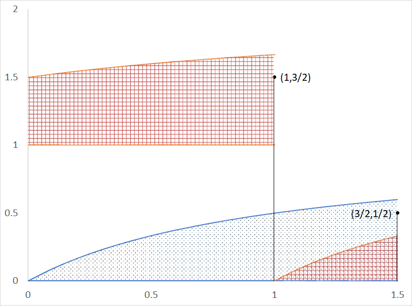
Let 𝒳={1,2}\mathcal{X}=\{1,2\}, with (1,2)≺(2,1)(1,2)\prec(2,1); also λ12​(y)=λ21​(y)=y1+y\lambda_{12}(y)=\lambda_{21}(y)=\frac{y}{1+y}, and λ~12​(y)=λ~21​(y)=sup(0,∞)|y1+y|=1\tilde{\lambda}_{12}(y)=\tilde{\lambda}_{21}(y)=\sup_{(0,\infty)}|\frac{y}{1+y}|=1 for all y≥0y\geq 0. Thus for every (i,j)∈𝒳2(i,j)\in\mathcal{X}_{2}, Λi​j(y)=[i−1,i−1+y1+y)\Lambda_{ij}(y)=[i-1,i-1+\frac{y}{1+y}). We further assume that Zl=(Xl,Yl)Z^{l}=(X^{l},Y^{l}) is the strong solution of (2.4)-(2.5) with above parameters and initial conditions (X0l,Y0l)=(l,𝟙{2}​(l))(X^{l}_{0},Y^{l}_{0})=(l,\mathds{1}_{\{2\}}(l)) for l=1,2l=1,2 respectively. Now fix a sample ω∈Ω\omega\in\Omega such that ℘⁡(ω)|[0,3/2]×[0,2]=δ(1,3/2)+δ(3/2,1/2)\wp(\omega)|_{[0,3/2]\times[0,2]}=\delta_{(1,3/2)}+\delta_{(3/2,1/2)}, the addition of two Dirac measures at (1,3/2)(1,3/2) and (3/2,1/2)(3/2,1/2) respectively.

Refer to caption
Figure 1. The tt and vv variables are plotted along horizontal and vertical axes. The point masses are shown by black dots. The intervals relevant for transitions of the first and second processes are plotted vertically and shown in blue and red respectively.

Then none of the processes has transition until time t=1t=1. Hence, for both l=1,2l=1,2,

X1−l​(ω)=l, and, ​Y1−l​(ω)=Y0l+1−∫(0,1)∫ℝgΛ​(Xu−l​(ω),Yu−l​(ω),v)​℘​(𝑑u,𝑑v)​(ω)=𝟙{2}​(l)+1=l.\displaystyle X^{l}_{1-}(\omega)=l,\,\textrm{ and, }\,Y^{l}_{1-}(\omega)=Y^{l}_{0}+1-\int_{(0,1)}\int_{\mathbb{R}}g_{\Lambda}(X^{l}_{u-}(\omega),Y^{l}_{u-}(\omega),v)\wp(du,dv)(\omega)=\mathds{1}_{\{2\}}(l)+1=l.

Then from (2.4)

X1l​(ω)=\displaystyle X^{l}_{1}(\omega)= X1−l​(ω)+∫ℝhΛ​(X1−l​(ω),Y1−l​(ω),v)​℘​({1},𝑑v)​(ω)=l+hΛ​(l,l,3/2).\displaystyle X^{l}_{1-}(\omega)+\int_{\mathbb{R}}h_{\Lambda}(X^{l}_{1-}(\omega),Y^{l}_{1-}(\omega),v)\wp(\{1\},dv)(\omega)=l+h_{\Lambda}(l,l,3/2).

Therefore, using (2.2) and the intervals Λ12​(1),Λ21​(2)\Lambda_{12}(1),\Lambda_{21}(2), we get X11​(ω)=1+(2−1)​𝟙[0,1/2)​(3/2)=1X^{1}_{1}(\omega)=1+(2-1)\mathds{1}_{[0,1/2)}(3/2)=1 and X12(ω)=2+(1−2)𝟙[1,1+2/3)(3/2)=1X^{2}_{1}(\omega)=2+(1-2)\mathds{1}_{[1,1+2/3)}(3/2)=1. Thus, t=1t=1 is a meeting time. However, this is not a merging time, because at t=3/2t=3/2, X1​(ω)X^{1}(\omega) and X2​(ω)X^{2}(\omega) separate, which is shown below. We note that until t=3/2t=3/2, X1​(ω)X^{1}(\omega) and X2​(ω)X^{2}(\omega) are at state 1 since t=0t=0, and t=1t=1 respectively. So, while the pre-transition state X3/2−l​(ω)X^{l}_{3/2-}(\omega) is 11 for each l=1,2l=1,2, the pre-transition ages Y3/2−1​(ω)Y^{1}_{3/2-}(\omega), and Y3/2−2​(ω)Y^{2}_{3/2-}(\omega) are 3/23/2 and 1/21/2 respectively. Consequently,

X3/2l​(ω)=\displaystyle X^{l}_{3/2}(\omega)= 1+∫ℝhΛ​(1,Y3/2−l​(ω),v)​℘​({3/2},𝑑v)​(ω)=1+𝟙Λ12​(Y3/2−l​(ω))​(1/2)={2,for ​l=11,for ​l=2\displaystyle 1+\int_{\mathbb{R}}h_{\Lambda}(1,Y^{l}_{3/2-}(\omega),v)\wp(\{3/2\},dv)(\omega)=1+\mathds{1}_{\Lambda_{12}(Y^{l}_{3/2-}(\omega))}(1/2)=\begin{cases}2,&\mbox{for }l=1\\ 1,&\mbox{for }l=2\end{cases}

since, 1/2∈Λ12​(3/2)=[0,3/21+3/2)=[0,3/5)1/2\in\Lambda_{12}(3/2)=[0,\frac{3/2}{1+3/2})=[0,3/5) and 1/2∉Λ12​(1/2)=[0,1/21+1/2)=[0,1/3)1/2\notin\Lambda_{12}(1/2)=[0,\frac{1/2}{1+1/2})=[0,1/3).

Theorem 3.3.

Assume (A3). Let Z1=(X1,Y1)Z^{1}=(X^{1},Y^{1}) and Z2=(X2,Y2)Z^{2}=(X^{2},Y^{2}) be as in Notation 2.2 where i≠ji\neq j. The probability of X1X^{1} and X2X^{2} meeting in the next transition is

∫0∞e−∫0y(λi(y1+t)+λj(y2+t))dt(λi​j(y1+y)+λj​i(y2+y))dy.\int_{0}^{\infty}e^{-\int_{0}^{y}(\lambda_{i}(y_{1}+t)+\lambda_{j}(y_{2}+t))dt}(\lambda_{ij}(y_{1}+y)+\lambda_{ji}(y_{2}+y))dy.

Proof. In this proof we will utilise that for every y′≥0y^{\prime}\geq 0 and y′′≥0y^{\prime\prime}\geq 0, ∪k≠iΛi​k(y′)\cup_{k\neq i}\Lambda_{ik}(y^{\prime}) is disjoint to ∪k≠jΛj​k(y′′)\cup_{k\neq j}\Lambda_{jk}(y^{\prime\prime}) when i≠ji\neq j. This is consequence of definitions of the intervals in (2.1), and (A3). Non-meeting event in the next transition of X1X^{1} and X2,X^{2}, happens in two ways.
Case 1: X1X^{1} has the first transition to a state which is different from X02X^{2}_{0} before X2X^{2} transits for the first time. This event can be written as ℰ:={XT1−1≠XT11,XT11≠XT12}\mathcal{E}:=\{X^{1}_{T_{1}-}\neq X^{1}_{T_{1}},X^{1}_{T_{1}}\neq X^{2}_{T_{1}}\}. We will make use of P⁡(ℰ∣ℱ0)=E⁡[P⁡(ℰ∣T1)∣ℱ0]P(\mathcal{E}\mid\mathcal{F}_{0})=E[P(\mathcal{E}\mid T_{1})\mid\mathcal{F}_{0}], and the expression of conditional density ηT1\eta_{T_{1}} of T1T_{1} given XT01=i,XT02=j,YT01=y1,YT02=y2X^{1}_{T_{0}}=i,X^{2}_{T_{0}}=j,Y^{1}_{T_{0}}=y_{1},Y^{2}_{T_{0}}=y_{2}. Clearly, P⁡(ℰ|T1=y)P(\mathcal{E}|T_{1}=y) is m1​(∪k∉{i,j}​Λi​k​(y1+y))m1​(∪k∉{i}​Λi​k​(y1+y)∪∪k∉{j}​Λj​k​(y2+y))\frac{m_{1}(\underset{k\notin\{i,j\}}{\cup}\Lambda_{ik}(y_{1}+y))}{m_{1}(\underset{k\notin\{i\}}{\cup}\Lambda_{ik}(y_{1}+y)\cup\underset{k\notin\{j\}}{\cup}\Lambda_{jk}(y_{2}+y))} =λi​(y1+y)−λi​j​(y1+y)λi​(y1+y)+λj​(y2+y)=\frac{\lambda_{i}(y_{1}+y)-\lambda_{ij}(y_{1}+y)}{\lambda_{i}(y_{1}+y)+\lambda_{j}(y_{2}+y)}. Moreover, ηT1​(y)=e−m2​(B)​(λi​(y1+y)+λj​(y2+y))\eta_{T_{1}}(y)=e^{-m_{2}(B)}(\lambda_{i}(y_{1}+y)+\lambda_{j}(y_{2}+y)), where B:=∪t∈[0,y)​({t}×((∪k∉{i}​Λi​k​(y1+t))∪(∪k∉{j}​Λj​k​(y2+t)))).B:=\underset{t\in[0,y)}{\cup}\left(\{t\}\times\left((\underset{k\notin\{i\}}{\cup}\Lambda_{ik}(y_{1}+t))\cup(\underset{k\notin\{j\}}{\cup}\Lambda_{jk}(y_{2}+t))\right)\right). Indeed, the event of no transition of X1X^{1} and X2X^{2} until first yy unit of time, is equivalent to {℘(B)=0}\{\wp(B)=0\}, the non-occurrence of Poisson point mass in BB. Clearly, P({℘(B)=0}∣XT01=i,XT02=j,YT01=y1,YT02=y2)P(\{\wp(B)=0\}\mid X^{1}_{T_{0}}=i,X^{2}_{T_{0}}=j,Y^{1}_{T_{0}}=y_{1},Y^{2}_{T_{0}}=y_{2}) is equal to e−m2​(B)e^{-m_{2}(B)}, and m2​(B)=∫0y(λi​(y1+t)+λj​(y2+t))​𝑑tm_{2}(B)=\int_{0}^{y}(\lambda_{i}(y_{1}+t)+\lambda_{j}(y_{2}+t))dt. Hence

P⁡(ℰ∣ℱ0)=\displaystyle P(\mathcal{E}\mid\mathcal{F}_{0})= ∫0∞P⁡(ℰ∣T1=y)​ηT1​(y)​𝑑y\displaystyle\int_{0}^{\infty}P(\mathcal{E}\mid T_{1}=y)\eta_{T_{1}}(y)dy
=\displaystyle= ∫0∞e−∫0y(λi(y1+t)+λj(y2+t))dt[λi(y1+y)−λi​j(y1+y)]dy.\displaystyle\int_{0}^{\infty}e^{-\int_{0}^{y}(\lambda_{i}(y_{1}+t)+\lambda_{j}(y_{2}+t))dt}[\lambda_{i}(y_{1}+y)-\lambda_{ij}(y_{1}+y)]dy. (3.2)

Similarly for Case 2, i.e., X2X^{2} has the first transition to a state, different from X01X^{1}_{0}, before X1X^{1} transits for the first time is given by,

P⁡(XT1−2≠XT12,XT12≠XT11∣ℱ0)\displaystyle P(X^{2}_{T_{1}-}\neq X^{2}_{T_{1}},X^{2}_{T_{1}}\neq X^{1}_{T_{1}}\mid\mathcal{F}_{0}) =∫0∞e−∫0y(λi(y1+t)+λj(y2+t))dt[λj(y2+y)−λj​i(y2+y)]dy.\displaystyle=\int_{0}^{\infty}e^{-\int_{0}^{y}(\lambda_{i}(y_{1}+t)+\lambda_{j}(y_{2}+t))dt}[\lambda_{j}(y_{2}+y)-\lambda_{ji}(y_{2}+y)]dy. (3.3)

Hence the total probability (denoted by a(i,j,y1,y2)′a^{\prime}_{(i,j,y_{1},y_{2})}) of not meeting in the next transition is sum of the probabilities appearing in (3.2), and (3.3).
Using ϕ1(y):=e−∫0y(λi(y1+t)+λj(y2+t))dt(λi(y1+y)+λj(y2+y))\phi_{1}(y):=e^{-\int_{0}^{y}(\lambda_{i}(y_{1}+t)+\lambda_{j}(y_{2}+t))dt}\left(\lambda_{i}(y_{1}+y)+\lambda_{j}(y_{2}+y)\right),

a(i,j,y1,y2)′\displaystyle a^{\prime}_{(i,j,y_{1},y_{2})} =∫0∞(ϕ1(y)−e−∫0y(λi(y1+t)+λj(y2+t))dt[(λi​j(y1+y)+λj​i(y2+y))])dy\displaystyle=\int_{0}^{\infty}\left(\phi_{1}(y)-e^{-\int_{0}^{y}(\lambda_{i}(y_{1}+t)+\lambda_{j}(y_{2}+t))dt}\left[(\lambda_{ij}(y_{1}+y)+\lambda_{ji}(y_{2}+y))\right]\right)dy (3.4)
=1−∫0∞e−∫0y(λi(y1+t)+λj(y2+t))dt(λi​j(y1+y)+λj​i(y2+y))dy\displaystyle=1-\int_{0}^{\infty}e^{-\int_{0}^{y}(\lambda_{i}(y_{1}+t)+\lambda_{j}(y_{2}+t))dt}{(\lambda_{ij}(y_{1}+y)+\lambda_{ji}(y_{2}+y))}dy

as ∫0∞ϕ1​(y)​𝑑y=1\int_{0}^{\infty}\phi_{1}(y)dy=1. Hence 1−a(i,j,y1,y2)′1-a^{\prime}_{(i,j,y_{1},y_{2})}, the probability of meeting of X1X^{1} and X2X^{2} in the next transition has the desired expression.∎

Definition 3.4.

Let Z1=(X1,Y1)Z^{1}=(X^{1},Y^{1}) and Z2=(X2,Y2)Z^{2}=(X^{2},Y^{2}) be the strong solutions of (2.4)-(2.5) with two different sets of initial conditions. Let 𝒫⁡(k,y)\mathcal{P}(k,y) denote the regular conditional probability of merging of X1X^{1} and X2X^{2} at a meeting time given meeting occurred in finite time, kk is the meeting state, and yy is the age of the chain which arrives at kk prior to the meeting time.

Theorem 3.5.

Assume (A3). Then

𝒫(k,y)=∫0∞e−∫0y′∑k′≠k(λk​k′(t)∨λk​k′(y+t))dt[∑k′≠kλk​k′(y′)∧λk​k′(y+y′)]dy′\displaystyle\mathcal{P}(k,y)=\int_{0}^{\infty}e^{-\int_{0}^{y^{\prime}}\underset{k^{\prime}\neq k}{\sum}(\lambda_{kk^{\prime}}(t)\vee\lambda_{kk^{\prime}}(y+t))dt}\left[\sum_{k^{\prime}\neq k}\lambda_{kk^{\prime}}(y^{\prime})\wedge\lambda_{kk^{\prime}}(y+y^{\prime})\right]dy^{\prime} (3.5)

where a∨b=max⁡(a,b)a\vee b=\max(a,b) and a∧b=min⁡(a,b)a\wedge b=\min(a,b).

Proof. Let t′t^{\prime} denote a meeting time of X1X^{1} and X2X^{2}. It is given that t′t^{\prime} is finite, with Xt′1=k=Xt′2X^{1}_{t^{\prime}}=k=X^{2}_{t^{\prime}}, Yt′1∧Yt′2=0Y^{1}_{t^{\prime}}\wedge Y^{2}_{t^{\prime}}=0 and Yt′1∨Yt′2=y>0Y^{1}_{t^{\prime}}\vee Y^{2}_{t^{\prime}}=y>0. Let ϑ\vartheta denote the duration both the processes stay at kk before either of them transit to some other state. Clearly, the event of no transition of X1X^{1} and X2X^{2} for next y′y^{\prime} unit of time after t′t^{\prime}, is equivalent to the event where no Poisson point mass belongs to the set B:=∪t∈[0,y′)​({t′+t}×∪k′∉{k}​(Λk​k′​(t)∪Λk​k′​(y+t)))B:=\underset{t\in[0,y^{\prime})}{\cup}\left(\{t^{\prime}+t\}\times\underset{k^{\prime}\notin\{k\}}{\cup}(\Lambda_{kk^{\prime}}(t)\cup\Lambda_{kk^{\prime}}(y+t))\right). Evidently, this event occurs with probability e−m2​(B)e^{-m_{2}(B)}, as m2m_{2} is the intensity of the Poisson random measure. Since, simultaneous occurrence of this event and the event of a Poisson point mass lying on the line segment {t′+y′}×∪k′∉{k}​(Λk​k′​(y′)∪Λk​k′​(y+y′))\{t^{\prime}+y^{\prime}\}\times\underset{k^{\prime}\notin\{k\}}{\cup}(\Lambda_{kk^{\prime}}(y^{\prime})\cup\Lambda_{kk^{\prime}}(y+y^{\prime})) is equivalent to the occurrence of {ϑ=y′}\{\vartheta=y^{\prime}\}, the expression of conditional density ηϑ\eta_{\vartheta} of ϑ\vartheta is given by ηϑ​(y′)=e−m2​(B)​m1​(∪k′∉{k}​Ak′​(y′))\eta_{\vartheta}(y^{\prime})=e^{-m_{2}(B)}m_{1}(\underset{k^{\prime}\notin\{k\}}{\cup}A_{k^{\prime}}(y^{\prime})), where Ak′​(y′):=Λk​k′​(y′)∪Λk​k′​(y+y′)A_{k^{\prime}}(y^{\prime}):=\Lambda_{kk^{\prime}}(y^{\prime})\cup\Lambda_{kk^{\prime}}(y+y^{\prime}) for every k′≠kk^{\prime}\neq k. As λ~i′​j′​(y)\tilde{\lambda}_{i^{\prime}j^{\prime}}(y) is set as constant ‖λi′​j′‖∞\|\lambda_{i^{\prime}j^{\prime}}\|_{\infty} for almost every yy (Assumption (A3)), due to the definitions of the intervals in (2.1), for almost every y≥0y\geq 0 and y′≥0y^{\prime}\geq 0 the collection {Ak′​(y′)}k′∈𝒳∖{k}\{A_{k^{\prime}}(y^{\prime})\}_{k^{\prime}\in\mathcal{X}\setminus\{k\}} is disjoint. Moreover, due to (A3) the left end points of the intervals Λk​k′​(y′)\Lambda_{kk^{\prime}}(y^{\prime}) and Λk​k′​(y+y′)\Lambda_{kk^{\prime}}(y+y^{\prime}) are common (see (2.1)). Thus the Lebesgue measures of Λk​k′​(y′)∪Λk​k′​(y+y′)\Lambda_{kk^{\prime}}(y^{\prime})\cup\Lambda_{kk^{\prime}}(y+y^{\prime}) and Λk​k′​(y′)∩Λk​k′​(y+y′)\Lambda_{kk^{\prime}}(y^{\prime})\cap\Lambda_{kk^{\prime}}(y+y^{\prime}) are λk​k′​(y′)∨λk​k′​(y+y′)\lambda_{kk^{\prime}}(y^{\prime})\vee\lambda_{kk^{\prime}}(y+y^{\prime}) and λk​k′​(y′)∧λk​k′​(y+y′)\lambda_{kk^{\prime}}(y^{\prime})\wedge\lambda_{kk^{\prime}}(y+y^{\prime}) respectively. Thus ηϑ(y′)=exp(−∫0y′∑k′≠k(λk​k′(t)∨λk​k′(y+t))dt)∑k′≠kλk​k′(y′)∨λk​k′(y+y′).\eta_{\vartheta}(y^{\prime})=\exp({-\int_{0}^{y^{\prime}}\underset{k^{\prime}\neq k}{\sum}(\lambda_{kk^{\prime}}(t)\vee\lambda_{kk^{\prime}}(y+t))dt})\sum_{k^{\prime}\neq k}\lambda_{kk^{\prime}}(y^{\prime})\vee\lambda_{kk^{\prime}}(y+y^{\prime}).

We consider two cases regarding the transition of X1X^{1} and X2X^{2}, at t′+ϑt^{\prime}+\vartheta which are (i) simultaneous, and (ii) non-simultaneous. Case (ii) implies that X1X^{1} and X2X^{2} will depart in the next transition. So, under case (ii), t′t^{\prime} is not a merging time. Consequently, case (i) is necessary for t′t^{\prime} to be the merging time. We show that case (i) is a sufficient condition too. We recall that at t′+ϑt^{\prime}+\vartheta the Poisson point mass (which is responsible for the transition) lies in only one of the members of the disjoint family {Ak′​(ϑ)}k′\{A_{k^{\prime}}(\vartheta)\}_{k^{\prime}} with probability one. Therefore, under case (i), at t′+ϑt^{\prime}+\vartheta, X1X^{1} and X2X^{2} enter into an identical state and the ages Y1Y^{1} and Y2Y^{2} become zero and therefore, the uniqueness of the SDE (2.4)-(2.5) implies merging at time t′t^{\prime}.

For case (i) to occur, the point mass must lie in {t′+ϑ}×∪k′∉{k}Λk​k′(ϑ)∩Λk​k′(y+ϑ)\{t^{\prime}+\vartheta\}\times\cup_{k^{\prime}\notin\{k\}}\Lambda_{kk^{\prime}}(\vartheta)\cap\Lambda_{kk^{\prime}}(y+\vartheta). On the other hand if the point mass lies in {t′+ϑ}×∪k′∉{k}(Ak′(ϑ)∖Λk​k′(ϑ)∩Λk​k′(y+ϑ))\{t^{\prime}+\vartheta\}\times\cup_{k^{\prime}\notin\{k\}}\left(A_{k^{\prime}}(\vartheta)\setminus\Lambda_{kk^{\prime}}(\vartheta)\cap\Lambda_{kk^{\prime}}(y+\vartheta)\right), then the transition at t′+ϑt^{\prime}+\vartheta is of case (ii). Hence, for almost every yy and y′y^{\prime}, the conditional probability of merging given ϑ=y′\vartheta=y^{\prime} is equal to ∑k′≠kλk​k′​(y′)∧λk​k′​(y+y′)∑k′≠k​(λk​k′​(y′)∨λk​k′​(y+y′))\frac{\sum_{k^{\prime}\neq k}\lambda_{kk^{\prime}}(y^{\prime})\wedge\lambda_{kk^{\prime}}(y+y^{\prime})}{\underset{k^{\prime}\neq k}{\sum}(\lambda_{kk^{\prime}}(y^{\prime})\vee\lambda_{kk^{\prime}}(y+y^{\prime}))}. Thus P(Xt1=Xt2,∀t≥t′∣{t′<∞},Xt′1=Xt′2=k,Yt′1∧Yt′2=0,Yt′1∨Yt′2=y)P\left(X^{1}_{t}=X^{2}_{t},\forall t\geq t^{\prime}\mid\{t^{\prime}<\infty\},X^{1}_{t^{\prime}}=X^{2}_{t^{\prime}}=k,Y^{1}_{t^{\prime}}\wedge Y^{2}_{t^{\prime}}=0,Y^{1}_{t^{\prime}}\vee Y^{2}_{t^{\prime}}=y\right) is equal to

∫0∞P(Xt1=Xt2,∀t≥t′∣{t′<∞},Xt′1=Xt′2=k,Yt′1∧Yt′2=0,Yt′1∨Yt′2=y,ϑ=y′)ηϑ(y′)dy′\displaystyle\int_{0}^{\infty}P\left(X^{1}_{t}=X^{2}_{t},\forall t\geq t^{\prime}\mid\{t^{\prime}<\infty\},X^{1}_{t^{\prime}}=X^{2}_{t^{\prime}}=k,Y^{1}_{t^{\prime}}\wedge Y^{2}_{t^{\prime}}=0,Y^{1}_{t^{\prime}}\vee Y^{2}_{t^{\prime}}=y,\vartheta=y^{\prime}\right)\eta_{\vartheta}(y^{\prime})dy^{\prime}
=∫0∞e−∫0y′∑k′≠k(λk​k′(t)∨λk​k′(y+t))dt(∑k′≠kλk​k′(y′)∧λk​k′(y+y′))dy′.\displaystyle=\int_{0}^{\infty}e^{-\int_{0}^{y^{\prime}}\underset{k^{\prime}\neq k}{\sum}(\lambda_{kk^{\prime}}(t)\vee\lambda_{kk^{\prime}}(y+t))dt}\left(\sum_{k^{\prime}\neq k}\lambda_{kk^{\prime}}(y^{\prime})\wedge\lambda_{kk^{\prime}}(y+y^{\prime})\right)dy^{\prime}.

This completes the proof. ∎

Remark 3.6.

It is interesting to note that for Markov special case, where the transition rate matrix λ\lambda is independent of the age variable yy, a direct calculation gives that 𝒫⁡(k,y)=1\mathcal{P}(k,y)=1. This makes Theorem 3.1, a corollary of the above theorem. On the other hand by considering the two-state semi-Markov chain given in Example 3.2, one can obtain for each k=1,2k=1,2, limy→∞𝒫⁡(k,y)=∫0∞e−y′​y′1+y′​d​y′<12​∫01e−y′​d​y′+∫1∞e−y′​d​y′=1+e−12<1\lim_{y\to\infty}\mathcal{P}(k,y)=\int_{0}^{\infty}e^{-y^{\prime}}\frac{y^{\prime}}{1+y^{\prime}}dy^{\prime}<\frac{1}{2}\int_{0}^{1}e^{-y^{\prime}}dy^{\prime}+\int_{1}^{\infty}e^{-y^{\prime}}dy^{\prime}=\frac{1+e^{-1}}{2}<1. This further clarifies that a meeting time for the flow in Example 3.2 need not be a merging time. Below we show that the chance of merging for a general semi-Markov chain increases to 1 as yy decreases to zero, provided that the transition rate is continuous at zero.

Proposition 3.7.

Assume (A3) and that y↦λ⁡(y)y\mapsto\lambda(y) is continuous at zero. As yy tends to zero, 𝒫⁡(k,y)\mathcal{P}(k,y) converges to 11.

Proof. From Theorem 3.5

limy→0𝒫⁡(k,y)\displaystyle\lim_{y\to 0}\mathcal{P}(k,y) =limy→0∫0∞e−∫0y′∑k′≠k(λk​k′(t)∨λk​k′(y+t))dt(∑k′≠kλk​k′(y′)∧λk​k′(y+y′))dy′.\displaystyle=\lim_{y\to 0}\int_{0}^{\infty}e^{-\int_{0}^{y^{\prime}}\underset{k^{\prime}\neq k}{\sum}(\lambda_{kk^{\prime}}(t)\vee\lambda_{kk^{\prime}}(y+t))dt}\left(\sum_{k^{\prime}\neq k}\lambda_{kk^{\prime}}(y^{\prime})\wedge\lambda_{kk^{\prime}}(y+y^{\prime})\right)dy^{\prime}.

Due to the continuity of λ\lambda in yy, the integrand converges pointwise to

ψ(y′):=∑k′≠kλk​k′(y′)exp(−∫0y′∑k′≠kλk​k′(t)dt).\psi(y^{\prime}):=\sum_{k^{\prime}\neq k}\lambda_{kk^{\prime}}(y^{\prime})\exp\left({-\int_{0}^{y^{\prime}}{\sum_{k^{\prime}\neq k}}\lambda_{kk^{\prime}}(t)dt}\right).

The integrand is also uniformly dominated by ψ\psi, which is integrable on [0,∞)[0,\infty). Indeed ∫[0,∞)ψ⁡(y′)​d​y′=1\int_{[0,\infty)}\psi(y^{\prime})dy^{\prime}=1. Thus the result follows using dominated convergence theorem. ∎

4. Eventual Meeting and Merging

It is important to note that the strict positivity of entries of the rate matrix, as assumed in this paper, implies irreducibility of the process. It is also known that mere irreducibility of a Markov chain does not ensure the convergence. However, the meeting event of two chains may take place even if the chains do not converge. The discrete time Markov chain on two states having zero probability of transition to the same state constitutes an example where chains with different initial states never meet due to its periodicity. Nevertheless, the same phenomena is untrue for its continuous time version. Indeed, if two such chains (Markov/semi-Markov), having bounded transition rate and driven by the same noise (the Poisson random measure) start from two different states, they meet surely at the next transition. In this paper, due to the consideration of processes having bounded transition rate, the discrete time scenario is excluded. Thus an ergodicity assumption is not needed for assuring eventual meeting. The next theorem establishes eventual meeting of Markov special case under finiteness assumption of the state space.

Theorem 4.1.

Let X1X^{1} and X2X^{2} be as in Theorem 3.1.

  1. (1)

    The conditional probability of meeting in the next transition given ℱ0\mathcal{F}_{0} is (λi​j+λj​i)λi+λj\frac{(\lambda_{ij}+\lambda_{ji})}{\lambda_{i}+\lambda_{j}}.

  2. (2)

    If 𝒳\mathcal{X} is finite, X1X^{1} and X2X^{2} eventually meet with probability 1.

Proof. Recall X01=iX^{1}_{0}=i, X02=jX^{2}_{0}=j, and the sequence {Tn}\{T_{n}\} from Notation 2.2. By applying Theorem 3.3 for the Markov special case, we can write the conditional probability of meeting in the next transition of X1X^{1} and X2X^{2}, given the initial conditions as

∫0∞e−∫0y(λi+λj)dt(λi​j+λj​i)dy=(λi​j+λj​i)(λi+λj)∫0∞e−(λi+λj)​y(λi+λj)dy=(λi​j+λj​i)(λi+λj).\displaystyle\int_{0}^{\infty}e^{-\int_{0}^{y}(\lambda_{i}+\lambda_{j})dt}(\lambda_{ij}+\lambda_{ji})dy=\frac{(\lambda_{ij}+\lambda_{ji})}{(\lambda_{i}+\lambda_{j})}\int_{0}^{\infty}e^{-(\lambda_{i}+\lambda_{j})y}(\lambda_{i}+\lambda_{j})dy=\frac{(\lambda_{ij}+\lambda_{ji})}{(\lambda_{i}+\lambda_{j})}.

Hence the part (1) is proved. Since, λi​j>0\lambda_{ij}>0 for all i≠ji\neq j and 𝒳\mathcal{X} is finite, mini,j⁡(λi​j+λj​i)λi+λj>0\min_{i,j}\frac{(\lambda_{ij}+\lambda_{ji})}{\lambda_{i}+\lambda_{j}}>0. Thus maxi,j⁡a(i,j)<1\max_{i,j}a_{(i,j)}<1 where a(i,j)a_{(i,j)} denotes the probability of not meeting in the next transition. Now since {Tn}\{T_{n}\} is a sequence of stopping times, using Theorem 2.1, we get

E[𝟙{X1Tn≠X2Tn}∣ℱTn−1]=a(XTn−11,XTn−12)≤maxi,ja(i,j)<1.\displaystyle E\left[\mathds{1}_{\{X^{1}_{T_{n}}\neq X^{2}_{T_{n}}\}}\mid\mathcal{F}_{T_{n-1}}\right]=a_{(X^{1}_{T_{n-1}},X^{2}_{T_{n-1}})}\leq\max_{i,j}a_{(i,j)}<1. (4.1)

The event of never meeting of processes X1X^{1} and X2X^{2} is identical to the repeated occurrence of {XTn1≠XTn2}\{X^{1}_{T_{n}}\neq X^{2}_{T_{n}}\} for all n≥1n\geq 1. Hence, using the fact (thanks to (A2)) that the chains experience infinitely many transitions with probability 1, the probability of never meeting, P(Xt1≠Xt2,∀t≥0∣ℱ0)P\left(X^{1}_{t}\neq X^{2}_{t},\forall t\geq 0\mid\mathcal{F}_{0}\right) matches with limN→∞P(∩n=1N{XTn1≠XTn2}∣ℱ0)\lim_{N\to\infty}P\left(\cap_{n=1}^{N}\{X^{1}_{T_{n}}\neq X^{2}_{T_{n}}\}\mid\mathcal{F}_{0}\right). Next if

E[∏n=1N𝟙{X1Tn≠X2Tn}∣ℱ0]≤maxi,ja(i,j)E[∏n=1N−1𝟙{X1Tn≠X2Tn}∣ℱ0],\displaystyle E\left[\prod_{n=1}^{N}\mathds{1}_{\{X^{1}_{T_{n}}\neq X^{2}_{T_{n}}\}}\mid\mathcal{F}_{0}\right]\leq\max_{i,j}a_{(i,j)}E\left[\prod_{n=1}^{N-1}\mathds{1}_{\{X^{1}_{T_{n}}\neq X^{2}_{T_{n}}\}}\mid\mathcal{F}_{0}\right], (4.2)

holds for all N≥1N\geq 1, using that repeatedly, we get

P(∩n=1N{XTn1≠XTn2}∣ℱ0)=E[∏n=1N𝟙{X1Tn≠X2Tn}∣ℱ0]≤(maxi,ja(i,j))NP\left(\cap_{n=1}^{N}\{X^{1}_{T_{n}}\neq X^{2}_{T_{n}}\}\mid\mathcal{F}_{0}\right)=E\left[\prod_{n=1}^{N}\mathds{1}_{\{X^{1}_{T_{n}}\neq X^{2}_{T_{n}}\}}\mid\mathcal{F}_{0}\right]\leq\left(\max_{i,j}a_{(i,j)}\right)^{N}

for all N≥1N\geq 1. The right side clearly vanishes as N→∞N\to\infty, and thus P(Xt1≠Xt2,∀t≥0∣ℱ0)P\left(X^{1}_{t}\neq X^{2}_{t},\forall t\geq 0\mid\mathcal{F}_{0}\right) is zero as desired, provided (4.2) holds. Finally (4.2) is shown using (4.1) below

E[∏n=1N𝟙{X1Tn≠X2Tn}∣ℱ0]\displaystyle E\left[\prod_{n=1}^{N}\mathds{1}_{\{X^{1}_{T_{n}}\neq X^{2}_{T_{n}}\}}\mid\mathcal{F}_{0}\right] =E[E[∏n=1N𝟙{X1Tn≠X2Tn}∣ℱTN−1]∣ℱ0]\displaystyle=E\left[E\left[\prod_{n=1}^{N}\mathds{1}_{\{X^{1}_{T_{n}}\neq X^{2}_{T_{n}}\}}\mid\mathcal{F}_{T_{N-1}}\right]\mid\mathcal{F}_{0}\right]
=E[(∏n=1N−1𝟙{X1Tn≠X2Tn})E[𝟙{X1TN≠X2TN}∣ℱTN−1]∣ℱ0]\displaystyle=E\left[\left(\prod_{n=1}^{N-1}\mathds{1}_{\{X^{1}_{T_{n}}\neq X^{2}_{T_{n}}\}}\right)E\left[\mathds{1}_{\{X^{1}_{T_{N}}\neq X^{2}_{T_{N}}\}}\mid\mathcal{F}_{T_{N-1}}\right]\mid\mathcal{F}_{0}\right]
≤maxi,ja(i,j)E[∏n=1N−1𝟙{X1Tn≠X2Tn}∣ℱ0]\displaystyle\leq\max_{i,j}a_{(i,j)}E\left[\prod_{n=1}^{N-1}\mathds{1}_{\{X^{1}_{T_{n}}\neq X^{2}_{T_{n}}\}}\mid\mathcal{F}_{0}\right]

for all N≥1N\geq 1. Hence the proof of part(2) is complete. ∎

In the above proof, the second part of the theorem has been proved using the first part. However, the former has been proved in Lemma 3.5 of [2] without utilizing part 1, under identical assumption in a different approach.

It is important to note that for ensuring almost sure eventual meeting, we have assumed finiteness of 𝒳\mathcal{X} in the above theorem, whereas in the proof we have used mini,j⁡(λi​j+λj​i)λi+λj>0\min_{i,j}\frac{(\lambda_{ij}+\lambda_{ji})}{\lambda_{i}+\lambda_{j}}>0 only. In the following lemma we show that under (A1), these conditions are equivalent.

Lemma 4.2.

Let λ\lambda be a transition rate matrix of a Markov chain obeying (A1). If 𝒳\mathcal{X} is infinite, infi,j​(λi​j+λj​i)λi+λj\underset{i,j}{\inf}\frac{\left(\lambda_{ij}+\lambda_{ji}\right)}{\lambda_{i}+\lambda_{j}} is zero.

Proof. Fix a j∈𝒳j\in\mathcal{X}. Since, due to Assumption (A1), ∑i=1∞λi<∞\sum_{i=1}^{\infty}\lambda_{i}<\infty, given ϵ>0\epsilon>0 there exists an iϵ,ji_{\epsilon,j} such that λi<ϵ​λj\lambda_{i}<\epsilon\lambda_{j} ∀i>iϵ,j.\forall i>i_{\epsilon,j}. So we get an inequality λi​j≤λi<ϵ​λj\lambda_{ij}\leq\lambda_{i}<\epsilon\lambda_{j} for all i>iϵ,ji>i_{\epsilon,j}. Using this inequality we have the following relation,

λi​j+λj​iλi+λj<ϵ​λj+λj​iλi+λj<ϵ​λj+λj​iλj=ϵ+λj​iλj,\frac{\lambda_{ij}+\lambda_{ji}}{\lambda_{i}+\lambda_{j}}<\frac{\epsilon\lambda_{j}+\lambda_{ji}}{\lambda_{i}+\lambda_{j}}<\frac{\epsilon\lambda_{j}+\lambda_{ji}}{\lambda_{j}}=\epsilon+\frac{\lambda_{ji}}{\lambda_{j}}, (4.3)

for all i>iϵ,ji>i_{\epsilon,j}. For each jj we also have λj=∑i∈𝒳∖{j}​λj​i<∞\lambda_{j}=\underset{i\in\mathcal{X}\setminus\{j\}}{\sum}\lambda_{ji}<\infty. Hence, there exists a ij,ϵ∗i^{*}_{j,\epsilon} such that for all i>ij,ϵ∗i>i^{*}_{j,\epsilon} we have λj​i<ϵ​λj\lambda_{ji}<\epsilon\lambda_{j}. Now, using (4.3), we get for each i>max⁡(iϵ,j,ij,ϵ∗),i>\max(i_{\epsilon,j},i^{*}_{j,\epsilon}),

λi​j+λj​iλi+λj<ϵ+ϵ​λjλj=2​ϵ.\displaystyle\frac{\lambda_{ij}+\lambda_{ji}}{\lambda_{i}+\lambda_{j}}<\epsilon+\frac{\epsilon\lambda_{j}}{\lambda_{j}}=2\epsilon.

Since ϵ\epsilon is arbitrary, the above implies that for each j∈𝒳j\in\mathcal{X},

limi→∞λi​j+λj​iλi+λj=0.\lim_{i\to\infty}\frac{\lambda_{ij}+\lambda_{ji}}{\lambda_{i}+\lambda_{j}}=0. (4.4)

Similarly by interchanging the roles of ii and jj in the above argument, one obtains

limj→∞λi​j+λj​iλi+λj=0\lim_{j\to\infty}\frac{\lambda_{ij}+\lambda_{ji}}{\lambda_{i}+\lambda_{j}}=0 (4.5)

for each i∈𝒳i\in\mathcal{X}. Hence from (4.4), and (4.5), we conclude infi,j​(λi​j+λj​iλi+λj)=0.\underset{i,j}{\inf}(\frac{\lambda_{ij}+\lambda_{ji}}{\lambda_{i}+\lambda_{j}})=0. ∎

Next we wish to investigate the eventual meeting event for semi-Markov family. Clearly, in view of Theorem 4.1(2), a condition like inf(i,j)∈𝒳2,y1,y2,y(λi​j​(y1+y)+λj​i​(y2+y))λi​(y1+y)+λj​(y2+y)>0\inf_{(i,j)\in\mathcal{X}_{2},y_{1},y_{2},y}\frac{(\lambda_{ij}(y_{1}+y)+\lambda_{ji}(y_{2}+y))}{\lambda_{i}(y_{1}+y)+\lambda_{j}(y_{2}+y)}>0 is needed for this purpose. However, finiteness of 𝒳\mathcal{X} is not enough to ensure that. We consider the following assumption.

  1. (A4)

    𝒳\mathcal{X} is finite and sup(i,j)∈𝒳2,y1≥0,y2≥0‖1−(λi​j(y1+⋅)+λj​i(y2+⋅))λi(y1+⋅)+λj(y2+⋅)‖L∞<1.\sup_{(i,j)\in\mathcal{X}_{2},y_{1}\geq 0,y_{2}\geq 0}\left\|1-\frac{\left(\lambda_{ij}(y_{1}+\cdot)+\lambda_{ji}(y_{2}+\cdot)\right)}{\lambda_{i}(y_{1}+\cdot)+\lambda_{j}(y_{2}+\cdot)}\right\|_{L^{\infty}}<1.

Theorem 4.3.

Assume (A1)-(A4) and that X1X^{1} and X2X^{2} are as in Notation 2.2. Then X1X^{1} and X2X^{2} eventually meet with probability 1.

Proof. Using ϕ2​(y):=1−(λi​j​(y1+y)+λj​i​(y2+y))λi​(y1+y)+λj​(y2+y)\phi_{2}(y):=1-\frac{(\lambda_{ij}(y_{1}+y)+\lambda_{ji}(y_{2}+y))}{\lambda_{i}(y_{1}+y)+\lambda_{j}(y_{2}+y)}, we rewrite (3.4) as

a(i,j,y1,y2)′\displaystyle a^{\prime}_{(i,j,y_{1},y_{2})} =∫0∞ϕ1​(y)​ϕ2​(y)​𝑑y≤‖ϕ1‖L1​‖ϕ2‖L∞=‖ϕ2‖L∞.\displaystyle=\int_{0}^{\infty}\phi_{1}(y)\phi_{2}(y)dy\leq\|\phi_{1}\|_{L^{1}}\|\phi_{2}\|_{L^{\infty}}=\|\phi_{2}\|_{L^{\infty}}.

Now by a direct application of (A4), we get that supremum of ‖ϕ2‖L∞\|\phi_{2}\|_{L^{\infty}} over all (i,j)∈𝒳2,y1≥0,y2≥0(i,j)\in\mathcal{X}_{2},y_{1}\geq 0,y_{2}\geq 0 is less than 1, which implies that

sup(i,j)∈𝒳2,y1≥0,y2≥0a(i,j,y1,y2)′<1.\sup_{(i,j)\in\mathcal{X}_{2},y_{1}\geq 0,y_{2}\geq 0}a^{\prime}_{(i,j,y_{1},y_{2})}<1. (4.6)

Again as in the proof of Theorem 4.1, the total probability of never meeting is the probability of intersection of occurrence of not meeting in next transition for every transition, and (A2) ensures almost sure infinite transitions. Moreover, since (Z1,Z2)(Z^{1},Z^{2}) is strong Markov (Theorem 2.1) and {Tn}n≥1\{T_{n}\}_{n\geq 1} are stopping times P({XTn1≠XTn2}∣ℱTn−1)=a(XTn−11,XTn−12,YTn−11,YTn−12)′P\left(\{X^{1}_{T_{n}}\neq X^{2}_{T_{n}}\}\mid\mathcal{F}_{T_{n-1}}\right)=a^{\prime}_{(X^{1}_{T_{n-1}},X^{2}_{T_{n-1}},Y^{1}_{T_{n-1}},Y^{2}_{T_{n-1}})} which is not more than the left side of (4.6). Therefore, in the similar line of the proof of Theorem 4.1, we get

E[∏n=1N𝟙{X1Tn≠X2Tn}∣ℱ0]≤(sup(i,j)∈𝒳2,y1≥0,y2≥0a(i,j,y1,y2)′)N\displaystyle E\left[\prod_{n=1}^{N}\mathds{1}_{\{X^{1}_{T_{n}}\neq X^{2}_{T_{n}}\}}\mid\mathcal{F}_{0}\right]\leq\left(\sup_{(i,j)\in\mathcal{X}_{2},y_{1}\geq 0,y_{2}\geq 0}a^{\prime}_{(i,j,y_{1},y_{2})}\right)^{N} (4.7)

and P(Xt1≠Xt2,∀t≥0∣ℱ0)=limN→∞E[∏n=1N𝟙{X1Tn≠X2Tn}∣ℱ0]P\left(X^{1}_{t}\neq X^{2}_{t},\forall t\geq 0\mid\mathcal{F}_{0}\right)=\lim_{N\to\infty}E\left[\prod_{n=1}^{N}\mathds{1}_{\{X^{1}_{T_{n}}\neq X^{2}_{T_{n}}\}}\mid\mathcal{F}_{0}\right]. This limit is zero from (4.6) and (4.7). Thus the probability of never meeting is zero. ∎ Under (A1)-(A4), the pair (X1,X2)(X^{1},X^{2}) not only surely meet, the expected number of transitions needed for meeting is also finite. A rather stronger result is shown below.

Theorem 4.4.

Assume (A1)-(A4) and that X1X^{1} and X2X^{2} are as in Notation 2.2. If NN denotes the number of collective transitions until the first meeting time of X1X^{1} and X2X^{2}, then E⁡[Nr]<∞E[N^{r}]<\infty for any r≥1r\geq 1.

Proof. For the sake of brevity, we write a(ZTn1,ZTn2)′a^{\prime}_{(Z^{1}_{T_{n}},Z^{2}_{T_{n}})} for a(XTn1,XTn2,YTn1,YTn2)′a^{\prime}_{(X^{1}_{T_{n}},X^{2}_{T_{n}},Y^{1}_{T_{n}},Y^{2}_{T_{n}})}, a notation that appears in the proof of Theorem 3.3. Since NN denotes the number of collective transitions until the first meeting time, using the above notation and (4.7), we get for all n≥0n\geq 0

P⁡(N=n+1)=\displaystyle P(N=n+1)= E[(∏r=1n𝟙{X1Tr≠X2Tr})E(𝟙{X1Tn+1=X2Tn+1}∣ℱTn)]\displaystyle E\left[\left(\prod_{r=1}^{n}\mathds{1}_{\{X^{1}_{T_{r}}\neq X^{2}_{T_{r}}\}}\right)E\left(\mathds{1}_{\{X^{1}_{T_{n+1}}=X^{2}_{T_{n+1}}\}}\mid\mathcal{F}_{T_{n}}\right)\right]
≤\displaystyle\leq (supz1,z2a(z1,z2)′)n​(1−infz1,z2a(z1,z2)′),\displaystyle\left(\sup_{z^{1},z^{2}}a^{\prime}_{(z^{1},z^{2})}\right)^{n}\left(1-\inf_{z^{1},z^{2}}a^{\prime}_{(z^{1},z^{2})}\right),

by following the convention that product and intersection of an empty family are 1 and empty set respectively. Thus the rt​hr^{th} raw moment, E⁡[Nr]E[N^{r}] is

∑n=1∞nr​P​(N=n)≤\displaystyle\sum_{n=1}^{\infty}n^{r}P(N=n)\leq (1−infz1,z2a(z1,z2)′)​(supz1,z2a(z1,z2)′)−1​∑n=1∞nr​(supz1,z2a(z1,z2)′)n.\displaystyle\left(1-\inf_{z^{1},z^{2}}a^{\prime}_{(z^{1},z^{2})}\right)\left(\sup_{z^{1},z^{2}}a^{\prime}_{(z^{1},z^{2})}\right)^{-1}\sum_{n=1}^{\infty}n^{r}\left(\sup_{z^{1},z^{2}}a^{\prime}_{(z^{1},z^{2})}\right)^{n}.

The infinite series on the right converges provided supz1,z2a(z1,z2)′<1\sup_{z^{1},z^{2}}a^{\prime}_{(z^{1},z^{2})}<1 which is ensured in (4.6) due to the assumption (A4). To be more precise, that series sum is expressed as L​i−r​(supz1,z2a(z1,z2)′)Li_{-r}(\sup_{z^{1},z^{2}}a^{\prime}_{(z^{1},z^{2})}) where L​ir​(z)Li_{r}(z) is polylogarithm function of order rr and with argument zz. Thus we conclude that NN has finite moments. ∎

We end this section with the final result below. That requires essential infimum of at least one entry of each row of λ\lambda to be nonzero.

Theorem 4.5.

Assume (A1)-(A4) and that X1X^{1} and X2X^{2} are as in Notation 2.2. Further assume that for each k∈𝒳k\in\mathcal{X} there is at least one k′∈𝒳∖{k}k^{\prime}\in\mathcal{X}\setminus\{k\} such that ‖λk​k′−1‖L∞<∞\|{\lambda_{kk^{\prime}}}^{-1}\|_{L^{\infty}}<\infty. Then X1X^{1} and X2X^{2} eventually merge with probability 1.

Proof. Since (A1)-(A4) hold, Theorem 4.3 ensures eventual meeting with probability 1. Hence 𝒯1<∞\mathcal{T}_{1}<\infty with probability 1, where 𝒯1\mathcal{T}_{1} denotes the first meeting time (see Definition 2.4 ). If 𝒯1\mathcal{T}_{1} is NMT (not a merging time), X1X^{1} and X2X^{2} separate at the next transition and again due to Theorem 4.3, they meet at 𝒯2\mathcal{T}_{2}, say, which is again finite almost surely. By repeating this argument, if X1X^{1} and X2X^{2} never merge, we obtain an infinite sequence {𝒯n}n\{\mathcal{T}_{n}\}_{n} of meeting times where each of them are finite almost surely. Using kn:=X𝒯n1=X𝒯n2k_{n}:=X^{1}_{\mathcal{T}_{n}}=X^{2}_{\mathcal{T}_{n}} and yn:=max⁡(Y𝒯n1,Y𝒯n2)y_{n}:=\max(Y^{1}_{\mathcal{T}_{n}},Y^{2}_{\mathcal{T}_{n}}), we get P⁡({𝒯n​ is NMT}∣ℱ𝒯n)=P⁡({𝒯n​ is NMT}∣kn,yn)=1−𝒫⁡(kn,yn)P\left({\{\mathcal{T}_{n}\textrm{ is NMT}\}}\mid\mathcal{F}_{\mathcal{T}_{n}}\right)=P\left({\{\mathcal{T}_{n}\textrm{ is NMT}\}}\mid k_{n},y_{n}\right)=1-\mathcal{P}(k_{n},y_{n}), since {𝒯n}n≥1\{\mathcal{T}_{n}\}_{n\geq 1} is a sequence of stopping times and (Z1,Z2)(Z^{1},Z^{2}) is strong Markov. Therefore,

E⁡[∏n=1N𝟙{𝒯n​ is NMT}]=\displaystyle E\left[\prod_{n=1}^{N}\mathds{1}_{\{\mathcal{T}_{n}\textrm{ is NMT}\}}\right]= E⁡[∏n=1N−1𝟙{𝒯n​ is NMT}​E​[𝟙{𝒯N​ is NMT}∣ℱ𝒯N]]\displaystyle E\left[\prod_{n=1}^{N-1}\mathds{1}_{\{\mathcal{T}_{n}\textrm{ is NMT}\}}E\left[\mathds{1}_{\{\mathcal{T}_{N}\textrm{ is NMT}\}}\mid\mathcal{F}_{\mathcal{T}_{N}}\right]\right]
≤(1−infk∈𝒳,y≥0𝒫⁡(k,y))​E​[∏n=1N−1𝟙{𝒯n​ is NMT}].\displaystyle\leq\left(1-\inf_{k\in\mathcal{X},y\geq 0}\mathcal{P}(k,y)\right)E\left[\prod_{n=1}^{N-1}\mathds{1}_{\{\mathcal{T}_{n}\textrm{ is NMT}\}}\right].

Since the event of never merging can be expressed as ∩n≥1{𝒯n is NMT}\cap_{n\geq 1}\{\mathcal{T}_{n}\textrm{ is NMT}\}, an upper bounded of its probability can be obtained by using the above inequality repeatedly, i.e.,

P(𝒯n is NMT,∀n≥1)=limN→∞E[∏n=1N𝟙{𝒯n​ is NMT}]≤limN→∞(1−infk∈𝒳,y≥0𝒫(k,y))N.\displaystyle P\left(\mathcal{T}_{n}\textrm{ is NMT},\forall n\geq 1\right)=\lim_{N\to\infty}E\left[\prod_{n=1}^{N}\mathds{1}_{\{\mathcal{T}_{n}\textrm{ is NMT}\}}\right]\leq\lim_{N\to\infty}\left(1-\inf_{k\in\mathcal{X},y\geq 0}\mathcal{P}(k,y)\right)^{N}. (4.8)

This confirms that the probability of never merging is zero, provided infk∈𝒳,y≥0𝒫⁡(k,y)>0\inf_{k\in\mathcal{X},y\geq 0}\mathcal{P}(k,y)>0. Since, (A3) holds, from Theorem 3.5,

𝒫⁡(k,y)≥\displaystyle\mathcal{P}(k,y)\geq ∫0∞e−∑k′≠k​‖λk​k′‖∞​y′​∑k′≠k‖λk​k′−1‖∞−1​d​y′\displaystyle\int_{0}^{\infty}e^{-\underset{k^{\prime}\neq k}{\sum}\|\lambda_{kk^{\prime}}\|_{\infty}y^{\prime}}\sum_{k^{\prime}\neq k}\|{\lambda_{kk^{\prime}}}^{-1}\|^{-1}_{\infty}dy^{\prime}
or, ​infk∈𝒳,y≥0𝒫⁡(k,y)≥\displaystyle\textrm{or, }\inf_{k\in\mathcal{X},y\geq 0}\mathcal{P}(k,y)\geq (∫0∞e−C​y′​d​y′)​min⁡∑k′≠kk∈𝒳⁡‖λk​k′−1‖∞−1.\displaystyle\left(\int_{0}^{\infty}e^{-Cy^{\prime}}dy^{\prime}\right)\min_{k\in\mathcal{X}}\sum_{k^{\prime}\neq k}\|{\lambda_{kk^{\prime}}}^{-1}\|^{-1}_{\infty}.

Since for each k∈𝒳k\in\mathcal{X}, there is a k′∈𝒳∖{k}k^{\prime}\in\mathcal{X}\setminus\{k\} such that ‖λk​k′−1‖L∞<∞\|{\lambda_{kk^{\prime}}}^{-1}\|_{L^{\infty}}<\infty, and 𝒳\mathcal{X} is finite, the right side of above inequality is positive. Thus infk∈𝒳,y≥0𝒫⁡(k,y)>0\inf_{k\in\mathcal{X},y\geq 0}\mathcal{P}(k,y)>0 as desired. ∎

5. Conclusion

In this paper we make use of a particular type of semimartingale representation of a class of semi-Markov processes. We have then studied various aspects of a pair of solutions having two different initial conditions. Several questions regarding the meeting and merging of stochastic flow of SMP have been answered by considering a solution pair. We have obtained explicit expressions of probabilities of many relevant events in terms of the transition rate matrix.

The study of eventual meeting and merging in Section 4 is carried out for finite state-space case. These results could be examined for certain infinite state cases, like birth-death processes, or more generally, where all entries of λ\lambda, except kk nearest neighbours of diagonal are zero. Apart from this, we also propose another extension. The present study which has been carried out for the time-homogeneous case, can further be investigated for the time non-homogeneous case. It is clear that the results of Section 4 cannot be extended in a straight forward manner for this general case. We wish to pursue further research in these directions.

Acknowledgement

The authors are grateful to Professors Mrinal K. Ghosh, and Gopal K. Basak for some helpful discussions. The authors also greatly appreciate some comments from Dr. Subhamay Saha, which helped in improving the readability. The suggestions of an anonymous referee have helped in improving the organization, presentation and focus of this paper significantly.

References