Theoretical and Practical Aspects of Space-Time DG-SEM Implementations
Abstract
We discuss two approaches for the formulation and implementation of space-time discontinuous Galerkin spectral element methods (DG-SEM). In one, time is treated as an additional coordinate direction and a Galerkin procedure is applied to the entire problem. In the other, the method of lines is used with DG-SEM in space and the fully implicit Runge-Kutta method Lobatto IIIC in time. The two approaches are mathematically equivalent in the sense that they lead to the same discrete solution. However, in practice they differ in several important respects, including the terminology used to describe them, the structure of the resulting software, and the interaction with nonlinear solvers. Challenges and merits of the two approaches are discussed with the goal of providing the practitioner with sufficient consideration to choose which path to follow. Additionally, implementations of the two methods are provided as a starting point for further development. Numerical experiments validate the theoretical accuracy of these codes and demonstrate their utility, even for 4D problems.
1 Introduction
Typically, partial differential equations are numerically treated with a method of lines ansatz; the spatial directions are discretized first, leaving the time variable continuous. The resulting system of ordinary differential equations is then solved using a numerical method for initial value problems.
An alternative ansatz is to treat the time dimension simply as another coordinate direction, and discretize the whole space-time problem simultaneously, resulting in a fully discrete numerical scheme [59]. This approach has several advantages: Moving boundaries can be treated more easily [74] and parallelization in time is made possible [31]. However, it also imposes new challenges since the temporal direction is special and needs to follow a causality principle: The solution at a given time is affected and determined only by the solution at earlier times, never the other way around. An overview of space-time computations in practical engineering applications during the last 25 years can be found in [73].
Here, we consider the discontinuous Galerkin spectral element method (DG-SEM); see e.g. [8] for an overview and [48] for a detailed exposition. These methods have been very successful for spatial discretizations as they are unstructured, of high order and are very suitable for high performance computing [51]. Further, DG-SEM fits the so-called Summation-By-Parts Simultaneous-Approximation-Term (SBP-SAT) framework [16, 33], implying stability for linear problems. Further, in the last decade, work within this framework has resulted in the development of entropy stable (i.e. nonlinearly stable) discretizations of arbitrarily high order [27, 26].
Our motivation to consider DG-SEM in a space-time formulation is twofold: Firstly, with a specific choice of numerical fluxes, entropy stability can be extended to incorporate the temporal discretization for hyperbolic conservation laws [29], thereby resulting in a nonlinearly stable, fully discrete scheme. Secondly, the formulation naturally allows for perfectly scaling parallelization in time, with a speedup equal to the number of discretization points within a time element. There are other approaches for parallelization in time that allow for much larger speedups, but need an initial factor of additional processors before giving any speedup at all [60].
There is a strong connection between DG discretizations in time and fully implicit Runge-Kutta (RK) methods: DG-SEM in time using an upwind numerical flux is equivalent to the Lobatto IIIC family of RK methods, in the sense that the two methods give the same numerical solution [10, 65]. This observation lends itself to two very different strategies for implementing DG-SEM in space and time. We can either use the method of lines with DG-SEM in space and Lobatto IIIC in time, or we can use space-time DG-SEM.
While mathematically equivalent, there are important differences between these two approaches:
- •
DG and RK methods have been developed largely independently. Hence, there is a language barrier between these communities, where different terminology is used, e.g. when it comes to order.
- •
The two approaches leads to different algebraic systems of linear or nonlinear equation. If solved exactly, these systems have the same solutions. However, in practice these solutions must be approximated, typically using iterative solvers. The interplay between iterative methods and the algebraic systems will in general be different, thus the two methods yield unequal numerical solutions.
- •
Implementing the two approaches lead to very different software structure, in particular if we wish to reuse existing software. This implies that various numerical tools and techniques may be more readily accessible in one implementation than the other, depending on whether the DG or the RK approach is chosen.
In this paper, we discuss these differences in detail so that practitioners can make an educated choice about which path to follow. Further, we present a code base for the two approaches that may be used as a basis for further development of the methods. In particular, we make use of the open source softwares Dune, the Distributed and Unified Numerics Environment, which is a modular toolbox for solving partial differential equations (PDEs) with grid-based methods [21]. We also make use of Assimulo [2], a solver package for initial value problems.
This paper is organized as follows: Following a brief literature review below, our target equation and choice of software is introduced in Section 2. In Section 3 we introduce the method of lines approach using DG-SEM with Lobatto IIIC for time stepping. In Section 4 the space-time DG-SEM is described. Throughout, code snippets are included to illustrate the details of the implementations. Theoretical aspects of the two approaches are discussed in Section 5. In particular, we demonstrate the mathematical equivalence of DG-SEM in time and Lobatto IIIC methods, and relate the terminology employed by the DG and RK communities. Practical aspects of the respective implementations are the subject of Section 6. Here we compare algorithmic and implementation specific requirements and merits of the two approaches. In Section 7 we present numerical experiments that validate some of our discussion points before we finish the article with some concluding remarks in Section 8. The Appendix A contains instructions on how to install the code discussed in this paper.
1.1 Further reading
For the practitioner who wishes to delve deeper into various aspects of the topics discussed in this paper, we here suggest a few places to start for further reading.
The book [48] provides much background material on spatial DG-SEM as well as a guide to its implementation. An overview of entropy stable DG-SEM is given in [34] and full mathematical detail is provided in [15]. The theory builds upon the SBP-SAT framework, reviews of which are found in [25, 72].
For a broad background on implicit Runge-Kutta methods, see [37]. An overview of the properties of DG-SEM and other SBP-SAT methods for time integration viewed from the Runge-Kutta perspective is given in [55]. An evaluation of fully implicit RK methods for use in computational fluid dynamics is given in [42], including discussions of how to solve the nonlinear algebraic systems.
2 Governing Equations and Simulation Software
We consider a general class of time dependent nonlinear advection-diffusion-reaction problems
| (1) |
for a vector valued function with components. Here, , . Suitable initial and boundary conditions are assumed to be available. and describe the convective and viscous fluxes respectively, and is a source term. We allow for the possibility that any of the coefficients in the partial differential equation (PDE) (1) depend explicitly on the spatial variable and on time , but to simplify the presentation we suppress this dependency in our notation.
For the discretization of (1) we consider two approaches: The first is a method of lines approach, in which the spatial differential operator is discretized using a DG-SEM approximation, yielding a system of ordinary differential equations (ODEs). This system is then solved using a time stepping scheme. In particular, we consider the Lobatto IIIC family of implicit Runge-Kutta methods.
The second approach is to apply the DG-SEM methodology to the entire equation (1), thereby obtaining a fully implicit DG space-time discretization.
In the following we will include code snippets to clarify the overall structure of the mathematical formulations at hand and to illustrate how the two approaches can be implemented in an existing code base. We utilize Dune [5], which is a free and open source software framework for the grid-based numerical solution of PDEs. Dune provides one of the most flexible and comprehensive grid interfaces available, allowing -dimensional grids, which we will use in this paper. Additionally, state-of-the-art features such as parallelization, grid adaptivity and load balancing, and moving grids are supported. From the variety of Dune modules available we will make use of the Python based front-end for Dune-Fem [22] and Dune-Fem-DG [19], which is able to handle weak forms of PDEs described in the Unified Form Language (UFL) [1]. As shown in the next section, the description of weak forms with UFL is straight forward and easy to use. Internally, PDEs described in UFL are translated into C++ code just-in-time, to ensure that the resulting simulation code is performant. For a more detailed description we refer to [22, 19] and the tutorial [20].
The implementation of the Lobatto IIIC method (see [53]) has been done in Assimulo [2], which is also a Python package that can be readily used together with Dune-Fem. Assimulo provides a high-level interface for a wide variety of classical and modern solvers of ordinary differential equations. e.g. SUNDIALS [40] and implicit Runge-Kutta solvers [36, 37]. The original codes, which are written in FORTRAN, C or Python, are wrapped into Assimulo keeping their original form, while the user only needs to interact with the Python interface, where the ODE and the initial condition of the problem need to be provided, as well as other additional information as e.g. the Jacobian, depending on the solver used. Existing solver options in Assimulo are for instance explicit and implicit Euler, Runge-Kutta34, RADAU5ODE, CVODE, IDA, ODASSL, LSODAR, GLIMDA.
Comments on how to install Dune-Fem-DG and Assimulo are found in Appendix A.
3 Method of Lines DG-SEM
In this section we describe the method of lines (MOL) approach to discretizing (1). A generic DG method is first presented, followed by the specifications needed to obtain the DG-SEM. Finally, the Lobatto IIIC time stepping method is specified.
3.1 DG-SEM in Space
Given a tessellation of the computational domain into elements with , consider the piecewise polynomial space
| (2) |
where is the space of polynomials whose degree do not exceed .
We let denote the set of intersections between all pairs of elements in and accordingly the set of all
intersections including the boundary of . In Dune, the following commands generate the tessellation and the space :
We seek an approximate solution by discretizing the spatial operator in (1). To this end we define for all test functions ,
| (3) |
Here, the element integrals are given by
| (4) |
where denotes the inner product of two second order tensors.
In the code this looks as follows:
The surface integrals are given by
| (5) | |||||
This formulation arises from considering the weak form of the problem: Replace by in (1), multiply by the test function and integrate the spatial terms by parts. Here, and are suitable numerical fluxes, imposed at the element interface . Further, and denote the average and jump of over ,
| (6) |
where and are neighboring elements over intersection and is outward pointing from element .
The corresponding code reads:
To obtain the DG-SEM we follow [50, 49]. First, we restrict our focus to cuboid meshes and map each to a reference element using an affine mapping. In the Dune implementation, the reference element is . This is due to a generic construction of reference elements of different shapes in arbitrary dimensions in Dune; see [23] for details.
In each spatial dimension, a set of Legendre-Gauss-Lobatto (LGL) nodes are introduced and a corresponding set of Lagrange basis polynomials are defined. The discrete solution takes the form
where the sum is taken over all tensor product LGL nodes in dimensions and is constructed as the product of Lagrange basis polynomials along each dimension.
This is achieved through the command
The convective and viscous fluxes are approximated using the interpolation
where is either or . A variety of implementations for and is provided by the dolfin_dg package (see [41]), which we use for the Euler equations.
Finally, the element and surface integrals in (4) and (5) are approximated using Gauss-Lobatto quadrature rules. The collocation of the quadrature with the LGL nodes results in a diagonal positive definite local mass matrix. The choice of a cuboid mesh and a tensor product formulation of the basis functions ensures that the global mass matrix remains diagonal positive definite and is consequently trivially invertible.
The convective numerical flux can be any appropriate numerical flux known for standard finite volume methods. We use the local Lax-Friedrichs (Rusanov) flux function
| (7) |
where is an estimate of the maximum wave speed on the interface . Other options are implemented in Dune-Fem-DG (cf. [18, 19]) as well.
A wide range of diffusion fluxes can be found in the literature (cf. [11] and references therein), however, only fluxes from the Interior Penalty family can currently be described in UFL due to the missing description and implementation in UFL of lifting terms needed for the other fluxes. For the Interior Penalty method the flux is chosen to be
| (8) |
with being the penalty parameter.
3.2 Temporal Discretization
After spatial discretization, we obtain a system of ODEs for the coefficient functions , which reads
| (9) |
Here, , where is defined in (3) and is the (diagonal) global mass matrix of the DG-SEM discretization. The initial data for (9) is given by the projection of onto .
Any Runge-Kutta method can in principle be used to solve (9). Explicit methods are easy to implement but suffer from severe time step restrictions for stiff systems.
Consider instead an implicit RK method with Butcher tableau
The stage equations of the RK method take the form
| (10) |
where the vector contains the intermediate solution stages and . Here, denotes the RK solution in the previous time step. The new solution is given by
| (11) |
Herein we consider a particular family of implicit RK methods, namely Lobatto IIIC [43, 53]. These methods are A-, L- and B-stable and are thus suitable for stiff and nonlinear problems. The order of the -stage Lobatto IIIC method is and the order of the individual stages is . However, this choice of method is also motivated by its equivalence to a space-time DG-SEM formulation, which is described in the next section. The Butcher tableaus for the 2-, 3- and 4-stage Lobatto IIIC methods are found in Appendix B.
The following code is an example how to use the Lobatto IIIC solvers in Assimulo:
4 Space-Time DG-SEM
We now consider DG-SEM applied to (1) with the time variable treated simply as an additional dimension. The result is space-time DG-SEM.
Defining the gradient and the new convective and viscous fluxes
we can rewrite (1) as a -dimensional problem over the space-time domain as
| (12) |
Given a tessellation of we introduce the piecewise polynomial space
| (13) |
Then the space-time DG-SEM discretization of (12) follows analogously to (4) and (5):
| (14) |
with the element integrals
| (15) |
and the surface integrals
| (16) | |||||
Here, and have analogous meanings to their spatial counterparts and . The numerical fluxes are given by
where is a simple upwind flux in time.
In our considered framework, (14) can be implemented quite nicely by increasing the
dimension and applying the above discussed modifications11
1
Note that for the 4D version ()
a UFL patch (see Appendix C) was added to introduce
the 4D reference elements to UFL code..
Remark 4.1.
It is of practical interest to generalize the space so that the time dimension may be discretized by polynomials of a different order than the spatial dimensions. We will henceforth refer to the number of temporal nodes in each element as so that the polynomial degree in time is . This notation contrasts standard DG terminology, where nodes are typically indexed from to . Additionally, note that this is the same notation used for the number of stages of the Lobatto IIIC method in Section 3. Stages are typically indexed from to . However, to minimize the use of notation and to make the connection between the two viewpoints clearer, we write to count the degrees of freedom within a time element, whether this pertains to the DG or RK interpretation.
After space-time discretization, the discrete solution takes the form . Here, the sum is taken over all tensor product LGL nodes in dimensions. The vector of coefficients is now given by
| (17) |
where contains all the spatial unknowns in the th time element.
The space-time discretization (14) can alternatively be derived by starting from (9) and discretizing in time with DG-SEM. Multiplying (9) by a test function and integrating over the th time element results in
We transform this equation to the reference element using the mapping , where . After integration by parts the resulting equation reads
We now follow the steps of DG-SEM, i.e. approximating and by interpolants
and the integrals by Gauss-Lobatto quadrature with nodes and weights . Using the cardinal property of the Lagrange basis polynomials , the resulting DG-SEM discretization becomes
| (18) |
Here, we have replaced the boundary terms with numerical fluxes . With DG-SEM in time, the numerical flux is always chosen as the upwind flux
| (19) |
where is the numerical solution from the previous time element. This choice leads to an entropy stable numerical scheme if the spatial terms are handled appropriately [29]. It also has the advantage of decoupling the temporal elements. Thus, (20) can be solved as a stand-alone nonlinear system on the th time element.
Defining the boundary, mass and differentiation matrices
we can write (18) in matrix form on each reference element as
| (20) |
where is the local temporal mass matrix and defines the corresponding stiffness matrix. Here, , where is given by (17) and is the th LGL node; see [33] for details. The operation denotes the Kronecker product and is the identity matrix whose dimension is given by the number of spatial nodes.
5 Theoretical Aspects of Space-Time DG-SEM
In this section we discuss important properties of the space-time DG-SEM, in particular the equivalence of the temporal discretization and the Lobatto IIIC family of Runge-Kutta methods. To make the connection between DG-SEM and Runge-Kutta methods clear, we consider the solution at the final point in the time element, i.e.
| (21) |
where . We will also make use of the vector . Following [10], we set out to show that , where is the numerical solution arising from the Lobatto IIIC method in (11), under the assumption that this equality holds in the previous (i.e. in the st) time element.
The DG-SEM discretization (20) constitutes a so called Summation-By-Parts (SBP) method [33], meaning that the following conditions are satisfied:
| (22) |
The SBP property (22) is at the heart of the connection of DG-SEM in time to implicit Runge-Kutta methods.
5.1 DG-SEM and Lobatto IIIC
SBP methods were historically developed to be used as spatial discretizations [52, 70]. For an overview of these techniques, see [72, 25]. In recent years, their use as time stepping schemes has been explored [62] and connections to implicit Runge-Kutta methods have been discovered [10]. Here we summarize the steps showing that (20) can be reformulated as an implicit RK method applied to the system of ODEs (9).
We begin by using the SBP property (22) in the second term of (20) and then multiplying by to obtain the so called strong form,
| (23) |
Note that and . Using (19), the second term in (23) can therefore be expressed as
Grouping together terms that multiply the solution , we rewrite (23) as
| (24) |
Next, we multiply (24) by . Upon doing this, first note that
which follows from observing that since by consistency. Thus, the following system arises:
| (25) | ||||
The equation system (25) should be compared with the stage equations (10) that arose from the MOL discretization using implicit RK. We see that the temporal DG-SEM discretization defines an RK method with coefficient matrix and nodes , where is the vector of LGL nodes. Further, the vector , which in the DG-SEM context contains the interpolation coefficients , has adopted the role of the stage vectors of the RK method.
To complete the transition from DG-SEM to RK, we compute the numerical solution at the final time node, . To this end we observe that the SBP property (22) gives the relation
so that
Consequently, multiplying (25) by yields
| (26) |
Comparing (26) with the solution (11) of the implicit RK method, we see that the vector in the Butcher tableau is related to the DG-SEM discretization by , and that the RK solution is simply the th component of the DG solution .
To summarize, a DG-SEM time discretization is equivalent to an implicit RK method whose Butcher tableau is defined in terms of the DG method as
| (27) |
The two methods yield two different nonlinear systems; for DG-SEM and RK they are respectively given by
| (28a) | ||||
| (28b) | ||||
These systems have the same solution since we can transition from (28a) to (28b) in a series of algebraic steps. More precisely, the connection is made by rewriting (28a) in strong form, then multiplying by .
Note that the latter step demands that is invertible. This is the case if and only if is null-space consistent, i.e. if [55]. This is known to hold for all [67, 54].
Finally, the Butcher tableau formed from (27) coincides with that of the Lobatto IIIC family of implicit Runge-Kutta methods. This follows from the use of LGL nodes and quadrature weights, together with a set of accuracy conditions satisfied by the two formulations [65]. We will detail these in the next section. The derivation above therefore shows that DG-SEM in time and the Lobatto IIIC methods are mathematically equivalent, and that we in fact have . The coefficients for the DG-SEM matrices with are listed in Appendix D.
5.2 Comparison of terminology
While DG-SEM in time and Lobatto IIIC are algebraically equivalent methods, they have been developed in different research communities and disparities have consequently arisen in terms of terminology. This pertains in particular to the notions of order and stability.
Beginning with RK methods, we take as our starting point the system of ODEs (9). The (classical) notion of order is defined as follows:
Definition 5.1.
The norm can be any vector norm and is called the global error.
The classical order of RK methods is determined by certain order conditions. To make the connection with DG-SEM as clear as possible, we present here a set of simplified conditions that are sufficient for the method to be of order [12]:
Theorem 5.2.
Suppose that an implicit Runge-Kutta method satisfies the conditions
- :
-
,
- :
-
,
- :
-
,
where and . Then the method is of order .
The conditions play a particularly important role in the context of stiff problems and have its own moniker:
Definition 5.3.
A Runge-Kutta method that satisfies the order conditions is said to have stage order .
The stage order of the RK method describes the accuracy with which the intermediate stages are approximated. We will delve into the meanings of the conditions , and shortly. However, first we summarize the various order concepts for Lobatto IIIC; see [37, Chapter IV.5].
Theorem 5.4.
The Lobatto IIIC method with stages satisfies , and . Consequently it has stage order and is of order .
We momentarily leave the RK viewpoint and focus on DG methods. DG-SEM was developed for spatial discretizations of time-dependent PDEs. Errors are measured in an norm over a spatial domain. For a discrete solution , this norm can be computed via the quadrature rule exactly:
| (29) |
The sum is taken over all elements and is the local spatial mass matrix on element . Assuming vanishingly small errors from the time discretization, the order of convergence measured in this norm is typically or , depending on the nature of problem (1), the choice of numerical fluxes, and sometimes on whether is odd or even [38, 77].
Conversely, when using DG-SEM as a time integration method, one works in the space . With an upwind flux in time, for sufficiently smooth and nonstiff problems, the order of convergence in this norm is [56]. This order is much smaller than the one of the Lobatto IIIC method, which requires some discussion.
There are several other order concepts in the DG literature. Here we follow [10] and relate these to the corresponding concepts in the RK framework.
- •
The order of the operator is the highest degree for which . The exponentiation should be interpreted elementwise, and we take as a definition. For DG-SEM we have .
Multiplying by as given in (27) and utilizing the fact that the first element in is zero, we see that the RK order condition actually describes precisely the order of the operator . A transformation of the reference element to is necessary in this step. In other words, the order of the operator is a concept identical to the stage order of the corresponding Lobatto IIIC method.
- •
The order of the norm/quadrature/mass matrix is the highest degree such that , i.e. for which exactly integrates polynomials. For DG-SEM, is a row vector with the weights of the Gauss-Lobatto quadrature rule and we consequently have .
Using (27) we note that the condition simply describes the order of the quadrature, although applied to rather than . Again, this amounts to a transformation from to .
- •
Pertinently, it turns out that the order of accuracy of the final component is [56], at least for smooth nonstiff problems. This superconvergence can be proven using the theory of dual consistent SBP methods [39]. Here it suffices to say that it is a consequence of the order of the quadrature and choosing the upwind numerical flux (19).
The superconvergence result pertaining to DG-SEM corresponds to the classical order of Lobatto IIIC as introduced in Definition 5.1. Note that this is a consequence of considering the pointwise error in time rather than .
To the best of our knowledge, conditions have no clear interpretation in the language of DG. Nevertheless, using the SBP property (22) and the diagonality of it is shown in [10] that is satisfied with , which is consistent with Theorem 5.4.
The convergence theory for RK methods relies on certain regularity properties of the problem being solved. In particular, it is assumed that the right-hand side of the system of ODEs (9) satisfies a one-sided Lipschitz condition,
| (30) |
where denotes some inner product and the corresponding norm. If , the problem is contractive. DG-SEM in time, and hence Lobatto IIIC, is stable for contractive problems, i.e. they are B-stable methods. Convergence for contractive problems is correspondingly known as B-convergence. B-convergence can be shown for Lobatto IIIC if , but in general not if if ; see [68] for details.
Regularity of the type (30) is not standard in the literature on spatial discretization using high order DG methods. Rather, estimates of the form are common. Such discretizations are referred to as semi-bounded, or in Runge-Kutta parlance, as monotonic. They arise particularly for discretizations of linear, homogeneous hyperbolic or parabolic problems, but also e.g. for the velocity components of the incompressible Navier-Stokes equations [61].
If , then semi-boundedness is a special case of contractivity and results on B-stability and B-convergence apply. However, for e.g. the equations of compressible flow, semi-boundedness must typically be replaced by entropy stability, i.e. regularity of the form . Here, is some convex function of referred to as an entropy [27, 26]. A convergence theory for implicit RK methods applied to entropy stable problems is desirable but currently appears to be missing from the literature.
6 Practical Aspects of Space-Time DG-SEM
In this section we discuss two archetypal implementations: On the one hand, the method of lines approach with Lobatto IIIC as discussed in Section 3 and on the other hand the space-time DG approach, as discussed in Section 4. We will refer to these as LoDG and STDG, respectively.
It is of course possible to produce a code that uses elements from both the LoDG and STDG formulation and thereby falls somewhere in between these approaches. However, here we adopt the point of view of a user who seeks to use an already available code base rather than producing a brand new solver.
Even though STDG and LoDG are mathematically equivalent methods, their respective implementations differ in several key aspects, each with particular requirements and accompanying merits. Here we will outline several such differences, and the choices a user will inevitable face when deciding on which implementation to select.
Several multi-dimensional DG-SEM solvers exist, such as Nektar++ [45], Fluxo, Flexi and the latest iteration Trixi [66] and others. In particular, this approach is popular for weather and climate prediction and has been used e.g. in NUMA [57] and HOMAM [58]. Thus, in the following discussion we assume that the user has access to a multi-dimensional DG solver for spatial discretization.
Our work here is based on the Dune-Fem framework, hence the challenges outlined below are flavoured by this choice. Depending on the software framework at hand, a user may find that one approach is easier to implement than the other.
6.1 STDG
As described in Section 4, the defining feature of STDG is the treatment of the -dimensional time-dependent problem as a -dimensional stationary problem.
Requirements: The problem description in the code must be extended to a -dimensional stationary PDE, which requires the software to be able to handle such problems. In particular, this includes the assembly of mass and stiffness matrices as well as having access to appropriate solvers for the resulting nonlinear system.
This new stationary PDE requires the use of different numerical fluxes in space and time; the temporal direction follows a causality principle, enforced by the upwind flux, which may not be the best choice for the spatial directions.
It is desirable to be able to choose different orders of accuracy in space and time, which then needs to be made possible in the DG code. In Dune this is implemented for certain DG spaces [35] but not yet available for the Lagrange basis used in this work.
The numerical solution should be accessible at specific time points in order for the user to visualize
intermediate results and the final solution.
For , this includes extracting -dimensional slices from -dimensional data sets. Related to this issue is the problem of -dimensional mesh generation. An example of how to handle this for the STDG ansatz
in Dune-Fem is found in Section 4.
Merits: If the requirements above are met, then existing software can be reused to solve the problem, which implies full control over the code. Moreover, only one code is needed. This code closely follows the mathematical derivation of the space-time method and may therefore be more intuitive than alternatives.
Due to the relatively simple adaption of an existing code for spatial problems of dimension , the STDG approach is fast for preliminary testing. An existing DG code is most likely optimized for computational resources and might even allow for parallelization in time by solving for several time steps at once.
In summary, this technique allows re-usability and full control over the code.
6.2 LoDG
The defining feature of LoDG is the method of lines approach outlined in Section 3. In this DG-SEM solver, each time step is solved individually.
Requirements: The (spatial) DG-SEM code needs to be coupled with an ODE solver with an implementation of a Lobatto IIIC method, most likely coming from another code. Difficulties may arise from the particular requirements of the two codes, such as interfaces for time and space adaptivity, parallelization etc.
The ODE solver might require input in a specific format not native to the DG code. Further, an efficient solution procedure may require information from the DG-SEM solver not directly available, such as the Jacobian of the spatial discretization.
Merits: No adaption of the DG code with respect to the PDE or its dimension is necessary. There are no additional difficulties arising in the treatment of -dimensional problems, and the resulting solution can be visualized in a straightforward way.
Most existing ODE solvers are optimized and equipped with several options, for instance adaptive time stepping. Intermediate results are easy to access and the order of accuracy in space and time can be chosen independently.
In summary, this technique provides flexibility and allows reuse of existing simulation workflows.
6.3 Algorithmic Aspects
In the following we suppose that we have overcome the most important challenges of the two approaches presented in the previous subsections. Thus we now have access to
In each time step, the LoDG code (approximately) solves (28b) while the STDG code solves (28a), or equivalently solves from (14). We now discuss the impact of choosing LoDG or STDG on a variety of algorithmic aspects.
Accessing time steps and stages: Accessing the numerical solution at a particular time is straightforward in most ODE solvers. The solution is computed either by aligning the step sizes with the target times or through accurate interpolation.
While it is possible to implement such techniques with STDG, they are unlikely to be available in a pre-existing DG code. Further, the code will return the numerical solution at all points in one (or several) time elements simultaneously. In fact, it is not obvious that the STDG code will be able to return in a simple way since this requires the extraction of a specific subset of coefficients from the numerical solution vector . Yet, this may be necessary e.g. for visualization, to use adaptive time stepping, or in case the solution needs to be filtered or otherwise modified between time steps. The solution can in principle be constructed using with , as was done in Section 5. However, this assumes that the ordering of the unknowns in is identical to the one used in that analysis. If not, must be suitably permuted into some matrix before application. Finding the appropriate permutation matrix may be a nontrivial task, in particular in 4D.
On the other hand, with STDG we have access to all intermediate time stages by default, something that may be challenging with LoDG. This may be useful to compute errors of the numerical solution and has the additional advantage of allowing visualization of the solution away from the main time steps.
Adaptive time-stepping: Adaptive time-stepping for RK methods is standard in modern software and thus will be available in an implementation of LoDG. It requires a way of estimating the numerical error in the next time step. This information is used to adapt the time step to fit a predefined tolerance. Embedding techniques use a vector to compute a second numerical solution from (11) whose accuracy is one order lower than that of . The difference can be used to estimate the local error without the need to solve the nonlinear system (28b) more than once. A detailed strategy for estimating the error and choosing the time step based on the embedding technique is available in [37, Chapter IV.8] for the Radau IIA method, but can be easily adapted to Lobatto IIIC [53]. .
An STDG code that follows the steps outlined in Section 4 will not have an embedded method. However, if the matrix can be found that extracts , then it is also possible to construct a matrix that extracts such that an embedding technique can be used. This procedure may be more invasive than desirable.
Alternatively, the numerical error can be estimated using Richardson extrapolation [36, Chapter II.4]. This procedure requires solving the nonlinear system (28a) three times; once with a step size and twice with a step size . The difference between the two solutions yields an error estimate. Due to its expense, this approach hardly seems feasible for a 4D problem.
Adaptive Mesh Refinement (AMR): Since STDG uses a 4D mesh it is straightforward to set up a system that accounts for multiple temporal elements at once, which is not possible with LoDG. This introduces the possibility of using AMR in time in addition to space; see [44, 17] and the references therein. Like with Richardson extrapolation, using AMR forces us to solve the nonlinear system multiple times. Additionally, the system now consists of multiple coupled time steps. However, the additional cost may be offset by two factors: Firstly, we expect that the number of degrees of freedom necessary to achieve a given accuracy is significantly reduced by the AMR. Secondly, parallelism can be employed in the temporal direction.
Space-time AMR is not likely to be simple to set up with commercially available software. However, if the initial hurdles can be circumvented, then it is in principle possible to use completely unstructured space-time grids with h/p-refinement. The technique requires a generator for unstructured cuboid meshes in 4D (tesseracts) [14] and a way of estimating the numerical error in the final time. Such tools have been developed for 4D simplex meshes in [76, 14], but appear to be missing for other mesh types.
Shock capturing and limiting: The DG spatial discretizations used with RK time stepping are stable when applied to linear problems such as linear hyperbolic systems. However, for nonlinear problems spurious oscillations occur near strong shocks or steep gradients. In this case the DG method requires some extra stabilization unless a first order scheme () is used that produces a monotonic structure in the shock region. For higher order schemes many approaches have been suggested to make this property available without introducing an excessive amount of numerical viscosity, which is a characteristic feature of first order schemes. Several approaches exist, including slope limiters, artificial diffusion (viscosity) techniques, and even a posteriori techniques and order reduction methods. A comprehensive literature list is presented in [69].
In Dune-Fem-DG [19], both limiter based approaches and artificial diffusion are available to stabilize a
DG scheme. The slope limiter based approach implemented in Dune-Fem-DG is coupled with a troubled cell
indicator which makes the overall scheme highly non-linear and therefore
not suitable for implicit methods, since the selection of troubled cells could
change between linear iterations and lead to divergence of the linear solver. On
the other hand, artificial diffusion approaches require a discretization of a diffusion term.
Stabilization diffusion coefficients only need to
be re-computed every time step. A standard approach is available in Dune-Fem-DG.
Thus, it is more suitable to apply artificial diffusion techniques
for problems where strong shocks occur.
Nonlinear solvers and preconditioning: The solutions of the nonlinear systems (28a) and (28b) must be approximated, typically by iterative methods for large systems. There have been a multitude of suggestions on how to design such methods; early solvers for implicit Runge-Kutta methods based on modified Newton iterations were introduced in [13] and [7]. A more optimized algorithm is described in [37], and many later developments use this as a starting point. These can be considered black box solvers in the sense that they do not utilize information about the spatial terms in the solution process.
Methods designed specifically for spatial DG discretizations and implicit Runge-Kutta methods are found in e.g. [63, 64]. Likewise, nonlinear solvers designed for space-time DG and FEM discretizations have been developed [47, 71].
Unless the user is willing to make the (possibly considerable) effort to develop and/or implement a nonlinear solver specifically designed for LoDG or STDG, the natural recourse is to use a black box solver. Efficiency gains can possibly be made by introducing a preconditioner designed for DG discretizations; see e.g. [9, 64, 46] for recent developments. However, attention must be payed to the fact that the systems (28a) and (28b) have different algebraic properties and therefore likely will respond differently to preconditioners and nonlinear solvers.
For the nonlinear LoDG system (28b), the Jacobian is given by
| (31) |
where contains the Jacobian of the spatial discretization. The solver in [37], and many recent developments that build upon it, instead use the mathematically equivalent
| (32) |
For the nonlinear STDG system (28a), the Jacobian is given by
| (33) |
Note from (27) that (32) arises by multiplying (31) by . This formulation is therefore very closely related to the STDG Jacobian (33). In fact, they only differ by an application of the SBP property (22) and a multiplication by the temporal mass matrix.
Consider the 1D linear advection equation discretized using a single element in space and time. With STDG, the discretization is generated using Dune. With LoDG, the spatial terms are generated with Dune whereas the temporal terms are set up manually as in Section 5. Figure 1 shows the sparsity patterns of the Jacobians using order 1,2 and 3 in space and time. In each figure quadruplet, the Jacobian (33) of STDG is shown in the top left and the Jacobian (31) of LoDG in the top right. In the bottom right, the alternative formulation (32) is shown.
The first thing to note is that the straightforward LoDG formulation leads to a dense discretization whereas STDG is sparse. The LoDG formulation using is also sparse. It has the same number of nonzero elements as STDG, although their distribution is different. The explanation for this lies in the ordering of the unknowns. With LoDG, the node order is lexicographic in the temporal direction. However, the space-time element generated by Dune is as shown in the bottom right of Figure 1, here with . This ordering is the result of a generic construction of the reference elements, which is based on a recursion over the spatial dimension starting at the -dimensional reference element, i.e. a point. This recursion also generates a natural ordering for the basis functions, starting with the basis functions located at points in an element and recursively down to the basis functions located inside the element. A detailed description of this construction is found in [23]. With a suitable permutation of the unknowns, the sparsity pattern of LoDG using coincides with STDG as seen in the bottom left of each figure quadruplet.
These observations suggest that the LoDG system (28b) is more expensive to work with than the STDG system (28a), and that the formulation (32) is a better choice. However, the interaction of particular preconditioners and solvers with these systems may also depend on the node ordering in ways that must be deduced through careful testing.


7 Experiments
We now perform a series of numerical tests. We start with solving the linear test equation to validate the convergence rates of the two solvers. A two-dimensional advection-diffusion test case follows, with the purpose of highlighting slight differences in the numerical solutions and particular challenges with respect to visualizing the solutions. Finally, the two and three dimensional Euler equations of gas dynamics are solved to demonstrate that both codes are capable of handling nonlinear space-time dynamics in multiple dimensions.
As mentioned previously, the spatial parts of both LoDG and STDG are generated using Dune-Fem. The temporal part of LoDG is implemented in Assimulo whereas Dune-Fem is used for the entire space-time discretization in STDG.
7.1 Validation of Convergence Rates
To verify that the temporal discretizations converge as expected we perform a simple test on the linear test equation,
| (34) | ||||
Python’s sparse linear solver is used to solve any algebraic systems arising from the discretizations. The experimental order of convergence (EOC) of the pointwise error is shown for LoDG and STDG in Table 1. Here, denotes the number of time steps/time elements and . Recall from Section 5 that the order of LoDG, and correspondingly the superconvergence of STDG, is . This is indeed what we observe in Table 1. With , the errors are approaching machine precision when , hence a drop in the convergence rate is seen in Table 1(b). The STDG appears to be more sensitive in this respect than LoDG. The same thing happens when and , as seen in Table 1(c).
| N | Lobatto | DG-SEM |
|---|---|---|
| 1.93 | 1.93 | |
| 1.97 | 1.97 | |
| 1.98 | 1.98 | |
| 1.99 | 1.99 | |
| 1.99 | 1.99 | |
| 1.99 | 1.99 |
| N | Lobatto | DG-SEM |
|---|---|---|
| 3.96 | 3.96 | |
| 3.98 | 3.98 | |
| 3.99 | 3.99 | |
| 3.99 | 4.01 | |
| 3.99 | 4.28 | |
| 4.05 | 0.47 |
| N | Lobatto | DG-SEM |
|---|---|---|
| 5.98 | 5.96 | |
| 6.64 | 4.22 |
We now repeat the experiment but measure the EOC via the norm . This type of error measurement is straightforward to perform with the STDG code. However, the LoDG implementation does not by default save the intermediate RK stages necessary to perform the computation of the error. We expect the EOC to be given by . Table 2 shows that this indeed is observed. For with time elements the convergence rate drops due to very small errors, as seen in Table 2(c). Again, STDG appears to be more sensitive to this phenomenon than LoDG.
| N | Lobatto | DG-SEM |
|---|---|---|
| 1.96 | 1.96 | |
| 1.98 | 1.98 | |
| 1.99 | 1.99 | |
| 2.0 | 2.0 | |
| 2.0 | 2.0 | |
| 2.0 | 2.0 |
| N | Lobatto | DG-SEM |
|---|---|---|
| 2.98 | 2.98 | |
| 2.99 | 2.99 | |
| 2.99 | 2.99 | |
| 3.0 | 3.0 | |
| 3.0 | 3.0 | |
| 3.0 | 3.0 |
| N | Lobatto | DG-SEM |
|---|---|---|
| 3.99 | 3.99 | |
| 4.0 | 4.0 | |
| 4.0 | 4.0 | |
| 4.0 | 4.0 | |
| 4.0 | 3.6 |
7.2 Advection-Diffusion
The next test case is the linear advection-diffusion problem in two dimensions;
| (35) | ||||||
We test both implementations for the rotating pulse problem with analytic solution
Here, , , , , and . The initial condition is given by and we apply periodic boundary conditions in space. The linear systems arising from the discretizations are solved using built-in routines in Dune and Assimulo. Thus, despite the mathematical equivalence of LoDG and STDG, we do not expect the two codes to yield identical solutions.
The numerical solutions obtained by the two codes with are shown in Figure 2. Here, a uniform mesh is used in space with . Time steps of uniform size are used throughout the simulation. With the problem is significantly under-resolved, leading to a smeared solution. As is increased, this phenomenon is reduced. To the eye, the numerical solutions using the two codes are barely distinguishable.


To get a more detailed comparison of the numerical results obtained by the two implementations we compare their spatial error in the final time point, . This time we vary the space-time grid with . The errors and the EOC are shown in Table 3. Notice that the errors are very similar, although not identical, testifying to the influence of the different solvers of the algebraic equations. Note also that the behaviour of the EOC is less clear than it was for the linear test equation. In this experiment we have refined space and time simultaneously, and therefore do not have a theoretical convergence result to rely on. The results indicate a convergence rate higher than , although not quite as high as .
| LoDG | STDG | LoDG | STDG | LoDG | STDG | |
| 8.94E-2 | 7.28E-2 | 4.45E-2 | 4.37E-2 | 2.68E-2 | 2.69E-2 | |
| 4.66E-2 | 4.46E-2 | 2.42E-2 | 2.41E-2 | 6.05E-3 | 6.04E-3 | |
| 3.49E-2 | 3.39E-2 | 5.36E-3 | 5.38E-3 | 4.92E-4 | 4.93E-4 | |
| 1.86E-2 | 1.84E-2 | 5.85E-4 | 5.94E-4 | 1.06E-5 | 9.88E-6 | |
| LoDG | STDG | LoDG | STDG | LoDG | STDG | |
| 0.9 | 0.7 | 0.9 | 0.9 | 2.1 | 2.2 | |
| 0.4 | 0.4 | 2.2 | 2.2 | 3.6 | 3.6 | |
| 0.9 | 0.9 | 3.2 | 3.2 | 5.5 | 5.6 | |
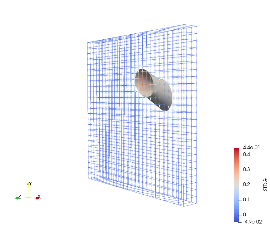
Finally, we highlight a feature of the STDG code that may be of use in certain situations. Since this code returns all points in a given time element (or equivalently, all intermediate RK stages in each time step), these can be visualized using a 3D plotting software, thereby obtaining a space-time visualization of the solution. These stages are usually discarded by ODE solvers for efficiency reasons. The visualization is done for a single time step in Figure 3. Here, the exact solution over the whole space-time domain is also shown for reference.



7.3 Euler Equations
A prime example for evolution equations are the Euler equations of gas dynamics. They are derived from the conservation of mass, momentum, and energy of a compressible inviscid fluid. In Eulerian coordinates they have the form:
| (36) | ||||||
where the vector of the conservative variables has the form
augmented with suitable boundary conditions (which are discussed in detail in [8]). Here, denotes the density of the fluid, the velocity, the internal energy, and the total energy. The convective flux function has for the form
where is the Kronecker delta. For example, choosing and directly using from (7.3) we obtain the three flux functions
We first consider the two-dimensional Euler equations with periodic boundary conditions and vortex initial condition
with vortex strength , Mach number , and .
The numerical solutions obtained by the two codes with are shown in Figure 4. Here, a uniform mesh on the space-time domain is used in space with . Time steps of uniform size are used throughout the simulation. Again, the problem is significantly under-resolved with , leading to a smeared solution. As is increased, this phenomenon is reduced. Some differences can be seen in the numerical results for the two implementations. This is likely caused by the fact that two different solvers, inherent to Assimulo and Dune respectively, are used for the nonlinear systems arising from the discretizations. Due to the differences between these solvers we can in general not expect identical numerical solutions despite the mathematical equivalence of the two algorithms.


To show the potential of our STDG code we present a 3D Euler test case with . We use periodic boundary conditions and a smooth bubble advection initial condition
with , and .
We consider the space-time domain and use a uniform mesh in space with and time steps of uniform size and throughout the simulation. The results have been computed on the LUNARC Aurora cluster at Lund University using Intel Xeon E5-2650 v3 processors and a Newton-GRMES solver with SOR preconditioning based on the PETSc library [3, 4]. On average we observe Newton iterations and about linear iterations per timestep for and about linear iterations per timestep for . The initial condition and the final time element of the density can be seen in Figure 5. They show that some care must be taken for the numerical solution to be properly resolved in time, with a time step size resulting in a smeared out solution with an error of in the last time point. When decreasing the time step to the numerical solution is more accurate with an error of . These results show the potential of the Dune code even for 4D problems. Recently, 4D problems have been taken into consideration [30], but to the best of our knowledge this is the first 4D DG-SEM implementation available publicly.


8 Conclusions
In this paper we have presented a comparison of the theoretical and practical aspects of two different space-time DG-SEM implementations. DG-SEM in time using an upwind numerical flux is equivalent to the Lobatto IIIC family of Runge-Kutta methods in the sense that they yield the same numerical solution when solved exactly. The two methods consequently have identical order, stability and convergence properties. However, since they emanate from different research communities, the terminology used to describe them are different. In this article we have made an effort to bridge this gap and to clarify the mathematical connections between the two methods.
Having two equivalent formulations of the same discretization raises the question of which path to take towards its implementation. Two strategies are immediately obvious: Either use the method of lines with DG-SEM in space and Lobatto IIIC in time (LoDG) or use a space-time DG-SEM approach (STDG). LoDG and STDG have been implemented using Dune-Fem and Assimulo and the codes are available as supplementary material to this paper; see Appendix A for details.
Despite the mathematical equivalence, there are important differences between the approaches. Not only are they described by different terminology in the literature. Additionally, the approaches lead to different systems of linear or nonlinear algebraic equations. When approximating their solutions using iterative methods, the solvers interact with these systems in different ways that are difficult to predict.
On the practical side, the two approaches lead to very different software structures that lend themselves to an assortment of opportunities and challenges. An overview of algorithmic capabilities has been given, that will be useful in different simulation contexts. These include adaptive time-stepping, adaptive mesh refinement, shock capturing, preconditioning, and other computational techniques. Some of these are likely to be more readily available in one implementation than the other, especially when reusing pre-existing code. The choice of an appropriate implementation thus depends on the needs of the user as well as on the software already available.
Several general conclusions about the two implementations can be drawn: For an STDG-type implementation, the code must be able to handle stationary 4D problems. It is desirable that the temporal dimension can be discretized with a different order of accuracy than the spatial dimensions. Further, adaptive time-stepping is nontrivial. On the other hand, this approach opens the door to parallelization in the time domain in ways that are usually not available. For problems in fewer than three spatial dimensions, software packages are already available and likely highly optimized.
For an LoDG-type implementation, black-box time-stepping routines are readily availble that implement Lobatto IIIC. Adaptive time-stepping is thus no issue, and the solution can easily be obtained at any desired intermediate times. There is no extension to 4D necessary and the order of accuracy in time can be set independently of the spatial discretization. On the other hand, this approach requires the coupling of two different codes. Parallelization in time also becomes less flexible.
Appendix A
There exist different ways to install Dune and Assimulo. Here, we only describe the simplest
and most straight forward way to install both, Dune and Assimulo, which is to
use a conda environment. Then the installation is done in the following way:
The space-time DG-SEM code is available online at https://gitlab.maths.lth.se/dune/spacetimelobattocode.
Appendix B
The Butcher tableaus for the -stage Lobatto IIIC methods with can be seen in Table 4.
Appendix C
This patch adds 4D simplex and cuboid reference elements to UFL needed for the
3D simulations. This patch is currently implemented in Dune-Fem and will
be discussed with the UFL community.
Appendix D
For we get
| (43) |
For we get
| (44) |
For we get
| (45) |
References
- [1] M. S. Alnæs, A. Logg, K. B. Ølgaard, M. E. Rognes, and G. N. Wells. Unified Form Language: A Domain-Specific Language for Weak Formulations of Partial Differential Equations. ACM Trans. Math. Softw., 40(2), 2014.
- [2] C. Andersson, C. Führer, and J. Åkesson. Assimulo: A unified framework for ODE solvers. Math. Comput. Simulat., 116(0):26 – 43, 2015.
- [3] S. Balay, S. Abhyankar, M. F. Adams, S. Benson, J. Brown, P. Brune, K. Buschelman, E. Constantinescu, L. Dalcin, A. Dener, V. Eijkhout, W. D. Gropp, V. Hapla, T. Isaac, P. Jolivet, D. Karpeev, D. Kaushik, M. G. Knepley, F. Kong, S. Kruger, D. A. May, L. C. McInnes, R. T. Mills, L. Mitchell, T. Munson, J. E. Roman, K. Rupp, P. Sanan, J. Sarich, B. F. Smith, S. Zampini, H. Zhang, H. Zhang, and J. Zhang. PETSc/TAO users manual. Technical Report ANL-21/39 - Revision 3.16, Argonne National Laboratory, 2021.
- [4] S. Balay, S. Abhyankar, M. F. Adams, S. Benson, J. Brown, P. Brune, K. Buschelman, E. M. Constantinescu, L. Dalcin, A. Dener, V. Eijkhout, W. D. Gropp, V. Hapla, T. Isaac, P. Jolivet, D. Karpeev, D. Kaushik, M. G. Knepley, F. Kong, S. Kruger, D. A. May, L. C. McInnes, R. T. Mills, L. Mitchell, T. Munson, J. E. Roman, K. Rupp, P. Sanan, J. Sarich, B. F. Smith, S. Zampini, H. Zhang, H. Zhang, and J. Zhang. PETSc Web page. https://petsc.org/, 2021.
- [5] P. Bastian, M. Blatt, M. Dedner, N.-A. Dreier, R. Engwer, Ch. Fritze, C. Gräser, C. Grüninger, D. Kempf, R. Klöfkorn, M. Ohlberger, and O. Sander. The Dune framework: Basic concepts and recent developments. Comput. Math. Appl., 81:75–112, 2021.
- [6] M. Behr. Simplex space–time meshes in finite element simulations. Int. J. Numer. Meth. Fl., 57(9):1421–1434, 2008.
- [7] T. A. Bickart. An efficient solution process for implicit Runge–Kutta methods. SIAM J. Numer. Anal., 14(6):1022–1027, 1977.
- [8] P. Birken. Numerical Methods for Unsteady Compressible Flow Problems. CRC Press, Boca Raton, London, New York, 2021.
- [9] P. Birken, G. J. Gassner, and L. M. Versbach. Subcell finite volume multigrid preconditioning for high-order discontinuous Galerkin methods. Int. J. Comput. Fluid. Dyn., 33(9):353–361, 2019.
- [10] P. D. Boom and D. W. Zingg. High-Order Implicit Time-Marching Methods Based on Generalized Summation-by-Parts Operators. SIAM J. Sci. Comput., 37:A2682–A2709, 2015.
- [11] S. Brdar, A. Dedner, and R. Klöfkorn. Compact and stable Discontinuous Galerkin methods for convection-diffusion problems. SIAM J. Sci. Comput., 34(1):263–282, 2012.
- [12] J. C. Butcher. Implicit Runge-Kutta Processes. Math. Comput., 18(85):50–64, 1964.
- [13] J. C. Butcher. On the implementation of implicit Runge-Kutta methods. BIT, 16(3):237–240, 1976.
- [14] P. C. Caplan, R. Haimes, D. L. Darmofal, and M. C. Galbraith. Four-dimensional anisotropic mesh adaptation. Comput. Aided Design, 129:102915, 2020.
- [15] M. H. Carpenter, T. C. Fisher, E. J. Nielsen, and S. H. Frankel. Entropy stable spectral collocation schemes for the Navier–Stokes equations: Discontinuous interfaces. SIAM J. Sci. Comput., 36(5):B835–B867, 2014.
- [16] M. H. Carpenter and D. Gottlieb. Spectral methods on arbitrary grids. J. Comput. Phys., 129(1):74–86, 1996.
- [17] Z. Chen, H. Steeb, and S. Diebels. A space-time discontinuous Galerkin method applied to single-phase flow in porous media. Computat. Geosci., 12(4):525–539, 2008.
- [18] A. Dedner, S. Girke, R. Klöfkorn, and T. Malkmus. The DUNE-FEM-DG module. Archive of Numerical Software, 5(1), 2017.
- [19] A. Dedner and R. Klöfkorn. Extendible and Efficient Python Framework for Solving Evolution Equations with Stabilized Discontinuous Galerkin Method. Comm. App. Math. Comp. Sci., 2021.
- [20] A. Dedner and R. Klöfkorn. The DUNE-FEM tutorial, 2022. https://dune-project.org/sphinx/content/sphinx/dune-fem/.
- [21] A. Dedner, R. Klöfkorn, and M. Nolte. Python bindings for the dune-fem module. Zenodo (Mar 2020), 2020.
- [22] A. Dedner, R. Klöfkorn, M. Nolte, and M. Ohlberger. A Generic Interface for Parallel and Adaptive Scientific Computing: Abstraction Principles and the DUNE-FEM Module. Computing, 90(3–4):165–196, 2010.
- [23] A. Dedner and M. Nolte. Construction of Local Finite Element Spaces Using the Generic Reference Elements. In A. Dedner, B. Flemisch, and R. Klöfkorn, editors, Advances in DUNE, pages 3–16, Berlin, Heidelberg, 2012. Springer Berlin Heidelberg.
- [24] L. T. Diosady and S. M. Murman. Tensor-product preconditioners for higher-order space–time discontinuous Galerkin methods. J. Comput. Phys., 330:296–318, 2017.
- [25] D. C. D. R. Fernández, J. E. Hicken, and D. W. Zingg. Review of summation-by-parts operators with simultaneous approximation terms for the numerical solution of partial differential equations. Comput. Fluids, 95:171–196, 2014.
- [26] T. C. Fisher and M. H. Carpenter. High-order entropy stable finite difference schemes for nonlinear conservation laws: Finite domains. J. Comput. Phys., 252:518–557, 2013.
- [27] T. C. Fisher, M. H. Carpenter, J. Nordström, N. K. Yamaleev, and C. Swanson. Discretely conservative finite-difference formulations for nonlinear conservation laws in split form: Theory and boundary conditions. J. Comput. Phys., 234:353–375, 2013.
- [28] M. Franciolini and S. M. Murman. Multigrid preconditioning for a space-time spectral-element discontinuous-Galerkin solver. In AIAA Scitech 2020 Forum, page 1314, 2020.
- [29] L. Friedrich, G. Schnücke, A. R. Winters, D. C. R. Fernández, G. J. Gassner, and M. H. Carpenter. Entropy Stable Space–Time Discontinuous Galerkin Schemes with Summation-by-Parts Property for Hyperbolic Conservation Laws. J. Sci. Comput., 80(1):175–222, 2019.
- [30] C. V. Frontin, G. S. Walters, F. D. Witherden, C. W. Lee, D. M. Williams, and D. L. Darmofal. Foundations of space-time finite element methods: Polytopes, interpolation, and integration. Appl. Numer. Math., 166:92–113, 2021.
- [31] M. J. Gander. 50 Years of Time Parallel Time Integration. In T. Carraro, M. Geiger, S. Körkel, and R. Rannacher, editors, Multiple Shooting and Time Domain Decomposition Methods, pages 69–113, Cham, 2015. Springer.
- [32] M. J. Gander and M. Neumüller. Analysis of a new space-time parallel multigrid algorithm for parabolic problems. SIAM J. Sci. Comput., 38(4):A2173–A2208, 2016.
- [33] G. J. Gassner. A skew-symmetric discontinuous Galerkin spectral element discretization and its relation to SBP-SAT finite difference methods. SIAM J. Sci. Comput., 35(3):A1233–A1253, 2013.
- [34] G. J. Gassner and A. R. Winters. A novel robust strategy for discontinuous Galerkin methods in computational fluid mechanics: Why? When? What? Where? Front. Phys., page 612, 2021.
- [35] C. Gersbacher. Higher-order discontinuous finite element methods and dynamic model adaptation for hyperbolic systems of conservation laws. Phd thesis, University of Freiburg, 2017.
- [36] E. Hairer, S. P. Nørsett, and G. Wanner. Solving Ordinary Differential Equations I. Springer, Berlin, Heidelberg, 2009.
- [37] E. Hairer and G. Wanner. Solving Ordinary Differential Equations II, volume 14 of Springer Series in Computational Mathematics. Springer, Berlin, Heidelberg, 2010.
- [38] J. S. Hesthaven and T. Warburton. Nodal discontinuous Galerkin methods: algorithms, analysis, and applications. Springer-Verlag New York, 2008.
- [39] J. E. Hicken and D. W. Zingg. Superconvergent functional estimates from summation-by-parts finite-difference discretizations. SIAM J. Sci. Comput., 33(2):893–922, 2011.
- [40] A. C. Hindmarsh, P. N. Brown, K. E. Grant, S. L. Lee, R. Serban, D. E. Shumaker, and C. S. Woodward. SUNDIALS: Suite of nonlinear and differential/algebraic equation solvers. ACM Transactions on Mathematical Software (TOMS), 31(3):363–396, 2005.
- [41] P. Houston and N. Sime. Automatic Symbolic Computation for Discontinuous Galerkin Finite Element Methods. SIAM J. Sci. Comput., 40(3):C327–C357, 2018.
- [42] A. Jameson. Evaluation of fully implicit Runge Kutta schemes for unsteady flow calculations. J. Sci. Comput., 73(2-3):819–852, 2017.
- [43] L. O. Jay. Lobatto methods. In B. Engquist, editor, Encyclopedia of Applied and Computational Mathematics, pages 817–826. Springer, Berlin, Heidelberg, 2015.
- [44] S. Jayasinghe, D. L. Darmofal, N. K. Burgess, M. C. Galbraith, and S. R. Allmaras. A space-time adaptive method for reservoir flows: formulation and one-dimensional application. Computat. Geosci., 22(1):107–123, 2018.
- [45] G. Karniadakis and S. Sherwin. Spectral/hp Element Methods for Computational Fluid Dynamics. Oxford University Press, Oxford, 2013.
- [46] J. Kasimir, L. M. Versbach, P. Birken, G. J. Gassner, and R. Klöfkorn. An Finite Volume Based Multigrid Preconditioner for DG-SEM for Convection-Diffusion. In 14th WCCM-ECCOMAS Congress 2020, volume 600, 2021.
- [47] C. M. Klaij, M. H. van Raalte, H. van der Ven, and J. J. van der Vegt. h-Multigrid for space-time discontinuous Galerkin discretizations of the compressible Navier-Stokes equations. J. Comput. Phys., 227(2):1024–1045, 2007.
- [48] D. A. Kopriva. Implementing Spectral Methods for Partial Differential Equations. Springer, Dordrecht, 2009.
- [49] D. A. Kopriva and G. Gassner. On the quadrature and weak form choices in collocation type discontinuous galerkin spectral element methods. J. Sci. Comput., 44:136–155, 2010.
- [50] D. A. Kopriva, S. L. Woodruff, and M. Y. Hussaini. Computation of electromagnetic scattering with a non-conforming discontinuous spectral element method. Int. J. Numer. Methods. Eng., 53(1):105–122, 2002.
- [51] N. Krais, A. Beck, T. Bolemann, H. Frank, D. Flad, G. Gassner, F. Hindenlang, M. Hoffmann, T. Kuhn, M. Sonntag, et al. Flexi: A high order discontinuous galerkin framework for hyperbolic–parabolic conservation laws. Comput. Math. Appl., 81:186–219, 2021.
- [52] H.-O. Kreiss and G. Scherer. Finite Element and Finite Difference Methods for Hyperbolic Partial Differential Equations. In C. de Boor, editor, Mathematical Aspects of Finite Elements in Partial Differential Equations, pages 195–212. Academic Press, London, 1974.
- [53] E. Lehsten. Implementation of 3 stage Lobatto IIIC into Assimulo package. Bachelor thesis, Lund University, 2021.
- [54] V. Linders. On an eigenvalue property of Summation-By-Parts operators. arXiv preprint arXiv:2201.01193, 2022.
- [55] V. Linders, J. Nordström, and S. H. Frankel. Properties of Runge-Kutta-Summation-By-Parts methods. J. Comput. Phys., 419:109684, 2020.
- [56] T. Lundquist and J. Nordström. The SBP–SAT technique for initial value problems. J. Comput. Phys., 270:86–104, 2014.
- [57] A. Müller, M. A. Kopera, S. Marras, L. C. Wilcox, T. Isaac, and F. X. Giraldo. Strong scaling for numerical weather prediction at petascale with the atmospheric model NUMA. Int. J. High. Perform. Comput. Appl., 33(2):411–426, 2019.
- [58] R. Nair, L. Bao, M. Toy, and R. Klöfkorn. A High-Order Multiscale Global Atmospheric Model. AIAA AVIATION Forum, 2016.
- [59] M. Neumüller. Space-Time Methods, volume 20 of Monograph Series TU Graz: Computation in Engineering and Science. TU Graz, 2013.
- [60] J. Nievergelt. Parallel methods for integrating ordinary differential equations. Commun. ACM, 7(12):731–733, 1964.
- [61] J. Nordström and C. La Cognata. Energy stable boundary conditions for the nonlinear incompressible Navier–Stokes equations. Math. Comput., 88(316):665–690, 2019.
- [62] J. Nordström and T. Lundquist. Summation-by-parts in time. J. Comput. Phys., 251:487–499, 2013.
- [63] W. Pazner and P.-O. Persson. Stage-parallel fully implicit Runge–Kutta solvers for discontinuous Galerkin fluid simulations. J. Comput. Phys., 335:700–717, 2017.
- [64] W. Pazner and P.-O. Persson. Approximate tensor-product preconditioners for very high order discontinuous Galerkin methods. J. Comput. Phys., 354:344–369, 2018.
- [65] H. Ranocha. Some notes on summation by parts time integration methods. Results Appl. Math., 1:100004, 2019.
- [66] H. Ranocha, M. Schlottke-Lakemper, A. R. Winters, E. Faulhaber, J. Chan, and G. Gassner. Adaptive numerical simulations with Trixi.jl: A case study of Julia for scientific computing, 08 2021.
- [67] A. A. Ruggiu and J. Nordström. On pseudo-spectral time discretizations in summation-by-parts form. J. Comput. Phys., 360:192–201, 2018.
- [68] J. Schneid. B-convergence of Lobatto IIIC formulas. Numer. Math., 51(2):229–235, 1987.
- [69] C.-W. Shu. High order WENO and DG methods for time-dependent convection-dominated PDEs: A brief survey of several recent developments. J. Comput. Phys., 316:598 – 613, 2016.
- [70] B. Strand. Summation by parts for finite difference approximations for d/dx. J. Comput. Phys., 110(1):47–67, 1994.
- [71] J. J. Sudirham, J. J. W. van der Vegt, and R. M. J. van Damme. Space-time discontinuous Galerkin method for advection-diffusion problems on time-dependent domains. Appl. Numer. Math., 56(12):1491–1518, 2006.
- [72] M. Svärd and J. Nordström. Review of summation-by-parts schemes for initial–boundary-value problems. J. Comput. Phys., 268:17–38, 2014.
- [73] T. E. Tezduyar and K. Takizawa. Space–time computations in practical engineering applications: A summary of the 25-year history. Comput. Mech., 63(4):747–753, 2019.
- [74] J. J. van der Vegt. Space-time discontinuous Galerkin finite element methods, pages 1–37. Von Karman Institute for Fluid Dynamics, Brussels, 2006.
- [75] L. M. Versbach, P. Birken, V. Linders, and G. Gassner. Local Fourier Analysis of a Space-Time Multigrid Method for DG-SEM for the Linear Advection Equation. arXiv preprint arXiv:2112.03115, 2021.
- [76] M. Yano and D. L. Darmofal. An optimization-based framework for anisotropic simplex mesh adaptation. J. Comput. Phys., 231(22):7626–7649, 2012.
- [77] Q. Zhang and C.-W. Shu. Error estimates to smooth solutions of runge–kutta discontinuous galerkin method for symmetrizable systems of conservation laws. SIAM J. Numer. Anal., 44(4):1703–1720, 2006.