A circuit-level protocol and analysis for twist-based lattice surgery
Abstract
Lattice surgery is a measurement-based technique for performing fault-tolerant quantum computation in two dimensions. When using the surface code, the most general lattice surgery operations require lattice irregularities called twist defects. However, implementing twist-based lattice surgery may require additional resources, such as extra device connectivity, and could lower the threshold and overall performance for the surface code. Here we provide an explicit twist-based lattice surgery protocol and its requisite connectivity layout. We also provide new stabilizer measurement circuits for measuring twist defects which are compatible with our chosen gate scheduling. We undertake the first circuit-level error correction simulations during twist-based lattice surgery using a biased depolarizing noise model. Our results indicate a slight decrease in the threshold for timelike logical failures compared to lattice surgery protocols with no twist defects in the bulk. However, comfortably below threshold (i.e. with CNOT infidelities below ), the performance degradation is mild and in fact preferable over proposed alternative twist-free schemes. Lastly, we provide an efficient scheme for measuring operators along boundaries of surface codes which bypasses certain steps that were required in previous schemes.
I Introduction
The surface code is a quantum error correcting code with a high threshold and which can be realised with two-dimensional hardware Dennis et al. 2002; Fowler et al. 2012. Other codes have been observed to have comparable thresholds for toy noise models Jochym-O’Connor and Laflamme 2014; Yoder et al. 2016; Chamberland et al. 2016; Chamberland et al. 2017; Chamberland et al. 2020a; Beverland et al. 2021, but when considering realistic circuit-level noise their performance (relative to the surface code) drops appreciably. The surface code’s high threshold can be partially attributed to the simplicity of its stabilizers and the circuits used to measure them. Realising the surface code requires measurements of pure -type and -type stabilizers involving no more than four qubits. These measurements can be performed using a depth-four sequence of two-qubit gates; the minimum we can hope for. Furthermore, choosing the right gate schedule can make the stabilizer measurement circuits immune to “hook” errors that effectively reduce the code distance. The moral here is that careful, circuit-level analysis of the microscopic details is crucial for a full understanding of the best route to fault-tolerant quantum computing.
Logical operations in two-dimensional surface code architectures can be performed by code deformation where the code stabilizers change over time, such as through braiding Raussendorf et al. 2006; Fowler et al. 2012 or lattice surgery Horsman et al. 2012; Litinski and Oppen 2018; Vuillot et al. 2019, with the latter being more resource efficient Fowler and Gidney 2018; Litinski 2019. The basic primitive in lattice surgery is a logical multi-qubit Pauli measurement, which when combined with logical ancilla states can be used to fault-tolerantly perform logical Clifford operations in addition to logical non-Clifford gates by teleportation. When measuring logical Paulis composed of and operators, the code is deformed with several surface code patches merged into a large patch, though locally the code stabilizers are unchanged. However, more generally, measurements involving Pauli operators are needed. Such measurements can be realised with twist-based lattice surgery Litinski and Oppen 2018, though this requires some weight-five measurements in addition to long range multi-qubit gates. The proposed twist-based approaches were presented abstractly, ignoring circuit-level implementation details and any related performance impacts.
Our work gives the first proposal for a circuit-level implementation of twist-based lattice surgery and numerically benchmarks the performance. In twist-based lattice surgery, we need to measure some longer range stabilizers that we call elongated rectangles and twist defects. To perform these measurements without increasing the circuit-depth (which would significantly degrade performance), we assume the hardware connectivity illustrated in Fig. 1. We say two qubits are connected when a two-qubit gate can be performed between these qubits. Standard surface code implementations have each qubit connected to four other qubits. In this work, we assume a minimal extension where some qubits are connected to eight other qubits. The cat-qubit based architecture of Ref. Chamberland et al. 2020b naturally provides this connectivity, and it could be produced in other architectures, though at the risk of additional cross-talk. Yoder and Kim proposed a twist-based scheme with lower weight measurements Yoder and Kim 2017, but they required a substantial change to the underlying surface code Yoder and Kim 2017 and did not use a homogeneous (translationally invariant) hardware. We leave open the question of whether twist-based lattice surgery can be realised using less connectivity within a homogeneous two-dimensional architecture.
To benchmark twist-based lattice surgery, we perform Monte Carlo simulations with a minimum-weight perfect matching (MWPM) decoding protocol (following the method of Ref. Chamberland and Campbell 2021) of and measurements. We perform our simulations for biased noise and rectangular surface codes since this enables us to perform larger simulations and these noise models are of recent interest Tuckett et al. 2019; Bonilla Ataides et al. 2021; Tuckett et al. 2020; Darmawan et al. 2021; Higgott and Breuckmann 2021; Chamberland et al. 2020b. We observe that the measurement of a logical operator has a higher logical failure rate relative to a comparable measurement of the same area. We attribute such differences to the presence of twist defects and elongated checks. The logical failure probability of these measurements is exponentially suppressed in the number of stabilizer measurement rounds used. Therefore, we can ask how many more rounds (and therefore time cost) is needed for a measurement to achieve the same logical fidelity as a measurement. We find, well below threshold (), the use of twists incurs only a small multiplicative time cost (less than for one of the studied noise models when ) since the twists are a small fraction of all possible fault locations. However, the twist defects are the weakest point and thus fail with a higher probability compared to other fault locations. Consequently, we find these multiplicative time costs increase as we approach the threshold.
In previous work Chamberland and Campbell 2021, we proposed an alternative twist-free lattice surgery scheme that replicated the computational power of Pauli measurements without the need for twist defects. However, this alternative strategy came with its own time cost. Therefore, a key conclusion of this work is that twist-based approaches outperform twist-free alternatives when operating comfortably below threshold, and under our connectivity assumptions along with the biased noise model used for the simulations. Twist-free lattice surgery may still prove useful in connectivity limited hardware or very close to threshold. Hardware afflicted by a different noise model than considered in this work might also benefit from twist-free lattice surgery.

II Lattice surgery with twist defects in the bulk
In this section, we describe our protocol for performing twist-based lattice surgery. In Section II.1, we provide a gate scheduling that can be used to measure an arbitrary number of Pauli operators using twist defects in the bulk. Fault-tolerant circuits for measuring stabilizers at twist defects are provided in Appendix A. In Section II.2, we will then compare the performance of a lattice surgery protocol for measuring to a protocol that does not require twist defects in the bulk. The Pauli is chosen for comparison since the measurement of both and require domain walls between the logical patches and the routing space. In what follows, the surface code encoding a logical qubit will be referred to as a logical patch. The extra space required to perform lattice surgery will be referred to as the routing space.
II.1 Gate scheduling for twist-based lattice surgery
Recall that in a lattice surgery protocol, mutli-qubit Pauli measurements between logical patches are performed by measuring a set of operators in the routing space between the logical patches. Such measurements (which correspond to gauge fixing Vuillot et al. 2019) merge the logical patches into one large surface code patch, and a subset of the stabilizers of the merged patch encode the parity of the logical multi-qubit Pauli measurement. A simple example for a and measurement is provided in Fig. 2.

Let be a multi-qubit Pauli operator that is to be measured using a lattice surgery protocol. If for all , then the standard surface code gate scheduling can be used to measure all the stabilizers during the lattice surgery protocol Tomita and Svore 2014. For instance, see the scheduling used for a logical measurement performed by lattice surgery in Fig. 2. With such a scheduling, all two-qubit gates can be applied in four time steps thus minimizing the number of idling qubit locations. One of the important features of the standard surface code gate scheduling circuits is that a weight-two error arising from a single fault will be perpendicular to the relevant logical operator thus preserving the surface code distance (i.e. the code will be guaranteed to correct any error arising from at most faults). By relevant logical operator, we mean that if the weight-two data-qubit error arising from a single fault is of the form and the minimum-weight representatives of form vertical strings, then will have support along horizontal strings. Similarly, will have support along vertical strings since the minimum-weight representatives of form horizontal strings.
Now suppose there exists at least one such that . In Fig.2d of Ref Litinski 2019, Litinski proposed measuring the operators as follows. First, logical patches are extended using qubits in the routing space such that the logical operator of the logical patch can be expressed along a horizontal boundary. The logical operator is then given by
| (1) |
where and are the minimum weights of the logical and operators of the logical patch. The operator can then be measured via gauge fixing by performing and -type stabilizer measurements between the extended logical patch and qubits in the routing space. The gauge-fixing step requires the measurement of mixed stabilizers which we refer to as domain walls. In addition, it requires the measurement of a weight-five operator operator containing a physical term. Such weight-five operators are referred to as twist defects. An important feature of our scheme is that when measuring multi-qubit Pauli’s involving operators, such measurements can be done directly, without first extending the logical patches. Using an extension step doubles the implementation time and uses additional routing space, thus making our direct approach more efficient. Further, we show in Appendix C that our direct approach for measuring Pauli operators is fault-tolerant using the gauge fixing formalism of Ref. Vuillot et al. 2019.
The presence of twist defects reduces the set of gate scheduling solutions that can be used for a twist-based lattice surgery protocol with minimal circuit depth. A valid gate scheduling for the measurement of via lattice surgery is shown in Fig. 2. The chosen gate scheduling ensures that all two-qubit gates can be applied in four time steps. Three different gate schedules are used, which are labelled A, B and C. The C schedule is only used in the routing space to the right of the twist defects. Note that the A, B and C schedules must follow a set of rules for how they can be tilled on the lattice in order to avoid scheduling conflicts or invalid schedules for performing the stabilizer measurements11 1 A valid schedule is one where all stabilizers are guaranteed to be measured as in the absence of faults. Further, if an error anticommutes with a stabilizer , then is guaranteed to be measured as .. For instance, a stabilizer measured using an A schedule cannot be adjacent to a stabilizer measured using a C schedule in the horizontal direction. If they were, qubits shared by both stabilizers would interact with two-qubit gates in the same time steps. On the other hand, C and A schedules can be adjacent to each other in the vertical direction (see the legend at the bottom of Fig. 2).

Unlike the standard surface code gate scheduling where all -type stabilizers use the A schedule and -type stabilizers use the B schedule (or vice-versa), the gate scheduling for measuring includes some regions where the A schedule is applied uniformly. Consequently, there will be single failures resulting in weight-two data qubit errors which are parallel to the logical or operators of the merged patch. For a given quantum algorithm, the and distances of logical patches are chosen such that a single logical data qubit error is very unlikely during the course of the entire computation. It is important to note that the merged lattices of a twist-based protocol with distances and for measuring operators will have and . In other words, the distances of the merged patches will be larger than the distances required for the logical patches prior to the merged. Therefore, even though our gate scheduling has the property that some weight-two errors arising from single failures will be parallel to or logical operators, the increased effective distances during lattice surgery protocols will ensure that and distances of the un-merged logical patches remain unchanged when performing twist-based lattice surgery, which we observe numerically. There are, however, some subtleties when performing twist-based lattice surgery that affect the minimum required value of (see Appendix B for details).
We now provide a generalization of the gate scheduling shown in Fig. 2 used for twist-based lattice surgery. In Fig. 3, we illustrate the gate scheduling required to measure the logical Pauli operator . The inclusion of a second pair of operators has the feature that all stabilizers of the merged patch in the routing space between the four twist defects are measured using the C schedule. As was the case in Fig. 2, the presence of twist defects requires the measurement of elongated stabilizers along vertical strips located between the twist defects in the routing space. In order to respect the nearest neighbor connectivity constraints imposed by many quantum hardware architectures, additional ancilla qubits need to be used to measure the elongated stabilizers and weight-five operators. However, an important feature of the circuit in Fig. 3 is that the gate scheduling imposes the need for different syndrome measurement circuits for the twist defects on the left strip compared to those on the right strip. More details are provided in Appendix A with the circuits shown in Fig. 7.
We remark that the gate scheduling shown in Fig. 3 can be extended to measure arbitrary multi-qubit Pauli operators such as the one shown in Fig. 4. In particular, Fig. 4 provides the minimal routing space requirements to perform arbitrary multi-qubit Pauli measurements for logical patches placed on a two-dimensional grid with qubits afflicted by a biased noise model. We assess the routing overhead by considering an individual unit cell of 4 logical patches shown in Fig. 4. Each unit cell uses physical qubits (which includes yellow and grey vertices) for the four logical patches and contains a total of physical qubits. The factor is the height of the unit cell. The factor is the width of the unit cell. Note with the width factor needs to account for the two patches and for the routing space between patches. It suffices to use a distance proportional to (rather than ) because when merging our lattice surgery patches, the effective distance is maintained. This leads to a multiplicative routing overhead of
| (2) |
where the approximation holds for large asymmetric codes . Eq. 2 corresponds to the asymptotic routing overhead since there is extra routing space required shown as green edge padding in Fig. 4. However, the cost of edge padding (as a fraction of total costs) vanishes with the number of logical qubits. The routing overhead can be reduced further if not every logical qubit is ready to participate in lattice surgery (e.g. see the core-cache model of Ref. Chamberland and Campbell 2021).
II.2 Performance comparison between twist-based and twist-free lattice surgery
Suppose we wish to measure a multi-qubit Pauli operator using lattice surgery. The parity of the multi-qubit Pauli measurement is given by a product of stabilizers in the routing space. For instance, for the measurement in Fig. 3, the parity of the measurement is given by the product of all -type stabilizers and twist defects in the routing space, in addition to domain wall stabilizers with the -component of the operator incident to the routing space. In what follows, we will refer to timelike failures as a collection of failure mechanisms which can result in the wrong parity outcome of a multi-qubit Pauli measurement implemented via lattice surgery. A logical timelike failure occurs when the incorrect parity of a multi-qubit Pauli is obtained after performing error correction over the full syndrome history of a lattice surgery protocol.
Due to timelike failures in addition to spacelike failures resulting in data qubit errors which anticommute with , the measurement of stabilizers in the routing space needs to be repeated times where is determined from the noise model and size of the computation. In particular, in a Pauli-based computation requiring the measurement of multi-qubit Pauli operators , in Ref.Chamberland and Campbell 2021 it was shown that can be chosen to satisfy where we require each multi-qubit Pauli measurement to fail with probability no greater than . Here is the worst case area of the routing space used for lattice surgery, are constants and quantifies the failure probability of all physical operations on the qubits.
The goal of this section is to quantify the relative performance of twist-based lattice surgery to a lattice surgery protocol free of twist defects. Such a comparison will allow us to quantify the extra algorithm runtime costs associated with twist defects. In particular, the weight-five stabilizers and elongated stabilizers have more fault locations compared to the weight-four stabilizers of the surface code and will thus make timelike failures more likely when measuring multi-qubit Pauli operators containing terms. In performing the comparison, we use the following biased circuit-level depolarizing noise model
- 1.
Each single-qubit gate location is followed by a Pauli error with probability and Pauli and errors each with probability .
- 2.
Each two-qubit gate is followed by a error with probability each, and a each with probability .
- 3.
With probability , the preparation of the state is replaced by . Similarly, with probability , the preparation of the state is replaced by .
- 4.
With probability , a single-qubit basis measurement outcome is flipped. With probability , a single-qubit -basis measurement outcome is flipped.
- 5.
Lastly, each idle gate location is followed by a Pauli with probability , and a error each with probability .
In performing our simulations, we consider two regimes for -basis measurement errors. The first is for and the second is for . All simulations are performed using , so that errors are one hundred times more likely than and errors. In what follows, we use a MWPM algorithm Edmonds 1965 on graphs with weighted edges to correct errors arising on the logical patches and in the routing space during a lattice surgery protocol. In particular, we use the decoding algorithm described in Section III of Ref.Chamberland and Campbell 2021.
For the twist-free simulation of lattice surgery, we consider a measurement due to the presence of domain walls at the boundaries of the logical patches and routing space. To gain some intuition on the expected scaling of the timelike logical failure rate (i.e. failures which result in the wrong interpretation of the parity of the measurement), suppose that the stabilizers of the merged patch for measuring via lattice surgery are measured times. Suppose further that starting in the first syndrome measurement round of the merged patch, a string of consecutive measurement errors occur on one of the stabilizers in the routing space encoding the parity of the measurement. Since the series of measurement errors begin in the first round, the inferred parity of the will be incorrect. Further, the minimum-weight path connecting the highlighted vertices22 2 A vertex of the matching graph used to perform MWPM encodes the parity of the measurement outcome of a given stabilizer in round . The vertex is highlighted if the measurement outcome of changes between consecutive syndrome measurement rounds and . will not pass through the parity vertices in the first syndrome round thus resulting in a logical timelike failure (see Ref.Chamberland and Campbell 2021 for more details). Additionally, the number of fault locations where timelike failures can occur is proportional to the area of the qubits in the routing space. As such, we propose the following ansatz for the timelike logical failure rate of a measurement:
| (3) |
where is the area of the routing space between the two domain walls (see Fig. 2), and are constants.
For the measurement of the operator , we expect a similar scaling to the one provided in Eq. 3. However, as can be seen in Figs. 2 and 3, measuring logical operators using twist defects results in narrow vertical strips of length which contain elongated stabilizers. Given the extra fault locations of both twist defects and elongated stabilizers, we consider the following ansatz for timelike logical failures
| (4) |
In Eq. 4, is given by Eq. 3 with replaced by the area of the routing space used for the measurement. In other words, the additional “cost” of performing twist-based lattice surgery is an additive error contribution proportional to the height containing twist defects and elongated stabilizers. For a multi-qubit Pauli measurement containing terms, we expect the timelike failure probability to scale as
| (5) |
for some constants where . In Eq. 5, we assume that the merged surface code patch for the measurement has the same area as the merged surface code patch for the measurement.
Performing full circuit-level simulations using the biased noise model and decoding algorithm described above, we obtained the following best fit polynomials describing the timelike logical failure rates using the ansatzes of Eqs. 3 and 4
| (6) |
and
| (7) |
The first term in Eqs. 6 and 7 can be used to extract the best fit polynomials for lattice surgery with a routing space area given by . In Fig. 5, we show how the polynomial in Eq. 6 fits the data obtained from our Monte Carlo simulations for various values of , and (with fixed ).
Now suppose that we wish to implement a quantum algorithm so that all lattice surgery operations fail with probability no more than . Hence we must have that which will fix the required value of for each multi-qubit Pauli measurement. Using the results of Eqs. 6 and 7, in Fig. 6, we plot the ratios for and . Here corresponds to the minimum value of such that . Note that in computing , the extension of the logical patch to obtain a horizontal boundary is done simultaneously with the gauge fixing step as explained in Appendix C. As such, counts all syndrome measurement rounds from the gauge fixing step until the round when the patches are split. Similarly, corresponds to the minimum value of such that for a lattice surgery patch where the routing space has the same area as the one used for a measurement. Hence, the ratio allows us to quantify the extra multiplicative time cost of measuring via lattice surgery using twist defects compared to a lattice surgery protocol for measuring which does not require the use of twist defects. A few remarks are in order.
First, the ratio is highly insensitive to the chosen values of , and . As such, the plots in Fig. 6 were obtained by fixing and . We chose the value since for the biased noise model considered here, it was shown in Ref.Chamberland and Campbell 2021 that was sufficient to implement the Hubbard model Hubbard 1963; Campbell 2021 for lattice sizes .
Second, comparing the results in Fig. 6a to those in Fig. 6b, it can be seen that higher measurement failure rates increase the runtime for performing lattice surgery with twist defects. Further, for physical noise rates , the ratio when . However, increases fairly quickly as approaches the regime which is near the threshold for logical timelike failures.
It can be seen in Fig. 6b that the ratio for increases when going from to . The absolute values of and are larger when . However, for both values of , we only require to achieve the desired target logical failure rates. As such, the fraction is larger when the absolute values of and decrease.
Lastly, we remark that for multi-qubit Pauli measurements requiring more than two terms, the ratios obtained in Fig. 6 would only increase in a meaningful way for very large values of when using the result of Eq. 5 due to the exponential scaling of the second term. As such, for the noise rates considered in Fig. 6, there could be rare cases where a multi-qubit Pauli measurement containing a very large number of terms would benefit from a twist-free approach such as the one considered in Chamberland and Campbell 2021.
III Conclusion
In Ref.Chamberland and Campbell 2021, the twist-free scheme for measuring multi-qubit Pauli operators containing terms results in an approximately slowdown in algorithm runtime due to the need to sequentially measure multi-qubit Pauli operators containing pure terms, followed by a multi-qubit Pauli measurement containing pure terms. Our results thus suggest that, assuming a hardware architecture satisfying the connectivity constraints described in Fig. 1, twist-based lattice surgery will outperform the twist-free version for physical noise rates . However, for noise rates close to the threshold value , we expect twist-free based lattice surgery to achieve lower algorithm runtime relative to lattice surgery protocols using twist defects to measure operators. An open question is whether high threshold surface code implementations are possible using homogeneous architectures and less connectivity as was assumed in Fig. 1.
The above conclusions also depend on the noise model. For instance, comparing Figs. 6a and 6b, it is clear that higher measurement failure rates results in longer measurements compared to measurements with an identical area. As such, for noise models where measurement and two-qubit gate failures are very high relative to other failure mechanisms, runtimes of twist-free lattice surgery protocols could potentially be smaller compared twist-based lattice surgery protocols.
Appendix A Stabilizer measurement circuits for twist defects in the bulk
In this appendix, we describe the two types of circuits used to measure elongated checks and the weight-five stabilizers corresponding to twist defects on both the left and right vertical strips in the routing space of Fig. 3. We presented one such example in Fig. 1 and here give a more general procedure. Such circuits are shown in Figs. 7a and 7b, where is the encoded state protecting the data during lattice surgery. and are Pauli operators with corresponding to the stabilizer being measured.
Without loss of generality, assume the data qubits is in an eigenstate of so that . For the circuit in Fig. 7a, it is straightforward to show that the state prior to the measurements is given by . The ancilla state is a eigenstate of with eigenvalue . As such, the product of the two -basis measurement outcomes of the ancilla qubits gives the stabilizer measurement outcome.
For the circuit in Fig. 7b, the state prior to the measurement is given by
| (8) |
which we can express as
| (9) |
Therefore, measuring the second ancilla qubit in the basis will reveal the desired eigenvalue. However, we also have a Pauli correction required depending on the value of the first ancilla qubit measured the basis.
Lastly, we point out that using flag based methods Chao and Reichardt 2018a; Chao and Reichardt 2018b; Chamberland and Beverland 2018; Tansuwannont et al. 2020; Reichardt 2020; Chamberland and Cross 2019; Chamberland and Noh 2020; Chamberland et al. 2020c; Chamberland et al. 2020a; Chao and Reichardt 2020; Tansuwannont and Leung 2021; Prabhu and Reichardt 2021; Postler et al. 2021; Tansuwannont and Leung 2021 to measure the elongated checks and weight-five twist defects would require an extra two-qubit gate between the ancillas instead of a single CNOT. As such, an extra idling time would be required resulting in slower algorithm runtimes.
Appendix B Minimum distance requirement of twist-based lattice surgery
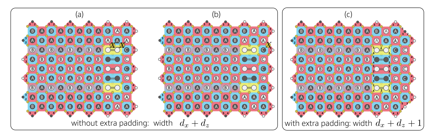
In this appendix, we show that twist-based lattice surgery protocols require extra padding to correct arbitrary errors arising from failures.
An example of a weight-one error being indistinguishable from a weight-two error (both arising from a single failure with probabilities proportional to ) for a lattice surgery protocol measuring is shown in Fig. 8. The lattices in Fig. 8(a) and (b) have width where and . The lattice in Fig. 8(c) has extra padding making its width . For the figure containing the lattices of width , consider first the lattice in Fig. 8(a). A weight-two data qubit error occurs during the first syndrome measurement round of the merged patch (i.e. the first syndrome measurement round when gauge fixing) due to a controlled- gate failure used for measuring the top twist defect. The error anticommutes with the weight-five yellow plaquette in addition to a blue weight-four -type stabilizer. However, the measurement outcome of the weight-five operator is random in the first round of the merge, and no change in measurement outcomes are observed in subsequent syndrome measurement rounds. As such, only the vertex associated with the weight-four -type stabilizer in the first round of the merge is highlighted. The observed syndrome measurement outcome is identical to the one that would be obtained if a weight-one error, as shown in Fig. 8(b), occurred during the first round of the merge. Since both a weight-one and weight-two errors result in the same syndrome measurement history, and , this example shows that a single failure occurring during the first syndrome measurement round when merging the surface code patches to measure can lead to a logical failure. However, by increasing the distance by one using extra padding, as shown in Fig. 8(c), such failure mechanisms can be distinguished.
More generally, suppose we perform lattice surgery using twist defects to measure operators and the initial logical patches prior to the merge have odd distance . In such settings, fewer than failures occurring during the first syndrome measurement round of the merged patch can result in a logical error. To ensure that up to failures never result in a logical failure, the logical patches can always be padded with an extra column of stabilizers thus increasing their distance by one. Depending on the noise bias and size of the quantum algorithm, the extra padding might not be necessary. For instance, the simulations performed in Section II.2 with a noise bias of used the odd distance which is sufficient for implementing the Hubbard model with lattice sizes . Further, even though for odd distances the logical failure probability scales as , the combinatorial coefficient is very small relative to the combinatorial coefficient of higher order failure mechanisms since only failures in the first round of the merged patch at very specialized regions near the twist defects can lead to a logical failure.

Appendix C Fault tolerance proof
Given a rectangular logical patch, in Ref. Litinski 2019 Litinski showed that the Pauli operator can be measured in several steps. We start with two separate surface code patches, the patch to be measured and a ancilla. The next step is to extend the patch by moving the corner to express a minimum weight representative of the logical operator along a straight line. Afterwords, a twist defect is used to measure with an ancilla prepared in a logical state. The last step implements destructive measurements on qubits in the ancilla region in order to return to the original code space. Litinski argued that the first and second steps require rounds of error correction, and all other steps require effectively zero time. We will refer to the second step as the extension step. If the extension step is required for a single logical measurement, it would seem natural to prefer this for and more general logical measurements. However, the extension step effectively doubles the execution time for lattice surgery and also demands additional routing space.
Here we argue that the extension step can be skipped while retaining all the fault-tolerance properties of lattice surgery at the phenomenological level. We borrow the gauge-fixing ideas of Ref. Vuillot et al. 2019 and apply them to the example of a measurement as sketched in Fig. 9.
The initial state of Fig. 9(a) has some set of stabilizers that includes all the stabilizer generators for the two logical patches. Note the data qubits in the routing space prepared in the state. Unconventionally, but crucial to our proof, we regard the Pauli for each qubit as being part of the stabilizer . This further allows us to choose an unusual representative for the and logical operators (each differs by a from relative to the standard representatives for and ).
The merged state of Fig. 9(b) illustrates the stabilizers during the merge step (having skipped any extension step). Multiplying the stabilizers with white vertices gives our representative for from the initial configuration and therefore these lattice surgery operations do measure the desired logical operator. If we had not included the single-qubit operators in , we would not have measured , so this is the key formal trick to prove fault-tolerance.
Lastly, Ref. Vuillot et al. 2019 prescribes that we consider the sub-system code with stabilizer and gauge group . The protocol is then (phenomenologically) fault-tolerant provided that this sub-system code retains the distance of the initial code. We illustrate the local generators for in Fig. 9(c). The logical operators for the sub-system code must commute with the stabilizer group and not be contained in the gauge group. Examining Fig. 9(c) one finds that the code distance is indeed maintained at for pure errors and at least for all other types of errors.
References
- Dennis et al. (2002) E. Dennis, A. Kitaev, A. Landahl, and J. Preskill, Topological quantum memory, Journal of Mathematical Physics 43, 4452 (2002).
- Fowler et al. (2012) A. G. Fowler, M. Mariantoni, J. M. Martinis, and A. N. Cleland, Surface codes: Towards practical large-scale quantum computation, Physical Review A 86, 032324 (2012).
- Jochym-O’Connor and Laflamme (2014) T. Jochym-O’Connor and R. Laflamme, Using concatenated quantum codes for universal fault-tolerant quantum gates, Phys. Rev. Lett. 112, 010505 (2014).
- Yoder et al. (2016) T. J. Yoder, R. Takagi, and I. L. Chuang, Universal fault-tolerant gates on concatenated stabilizer codes, Phys. Rev. X 6, 031039 (2016).
- Chamberland et al. (2016) C. Chamberland, T. Jochym-O’Connor, and R. Laflamme, Thresholds for universal concatenated quantum codes, Phys. Rev. Lett. 117, 010501 (2016).
- Chamberland et al. (2017) C. Chamberland, T. Jochym-O’Connor, and R. Laflamme, Overhead analysis of universal concatenated quantum codes, Phys. Rev. A 95, 022313 (2017).
- Chamberland et al. (2020a) C. Chamberland, A. Kubica, T. J. Yoder, and G. Zhu, Triangular color codes on trivalent graphs with flag qubits, New Journal of Physics 22, 023019 (2020a).
- Beverland et al. (2021) M. E. Beverland, A. Kubica, and K. M. Svore, Cost of universality: A comparative study of the overhead of state distillation and code switching with color codes, PRX Quantum 2, 020341 (2021).
- Raussendorf et al. (2006) R. Raussendorf, J. Harrington, and K. Goyal, A fault-tolerant one-way quantum computer, Annals of Physics 321, 2242 (2006).
- Horsman et al. (2012) C. Horsman, A. G. Fowler, S. Devitt, and R. Van Meter, Surface code quantum computing by lattice surgery, New J. Phys. 14, 123011 (2012).
- Litinski and Oppen (2018) D. Litinski and F. v. Oppen, Lattice Surgery with a Twist: Simplifying Clifford Gates of Surface Codes, Quantum 2, 62 (2018).
- Vuillot et al. (2019) C. Vuillot, L. Lao, B. Criger, C. G. Almudéver, K. Bertels, and B. M. Terhal, Code deformation and lattice surgery are gauge fixing, New J. Phys. 21, 033028 (2019).
- Fowler and Gidney (2018) A. G. Fowler and C. Gidney, Low overhead quantum computation using lattice surgery, arXiv preprint arXiv:1808.06709 (2018).
- Litinski (2019) D. Litinski, A Game of Surface Codes: Large-Scale Quantum Computing with Lattice Surgery, Quantum 3, 128 (2019).
- Chamberland et al. (2020b) C. Chamberland, K. Noh, P. Arrangoiz-Arriola, E. T. Campbell, C. T. Hann, J. Iverson, H. Putterman, T. C. Bohdanowicz, S. T. Flammia, A. Keller, G. Refael, J. Preskill, L. Jiang, A. H. Safavi-Naeini, O. Painter, and F. G.S.L. Brandao, Building a fault-tolerant quantum computer using concatenated cat codes, arXiv preprint arXiv:2012.04108 (2020b).
- Yoder and Kim (2017) T. J. Yoder and I. H. Kim, The surface code with a twist, Quantum 1, 2 (2017).
- Chamberland and Campbell (2021) C. Chamberland and E. T. Campbell, Universal quantum computing with twist-free and temporally encoded lattice surgery, arXiv e-prints (2021), arXiv:2109.02746 .
- Tuckett et al. (2019) D. K. Tuckett, A. S. Darmawan, C. T. Chubb, S. Bravyi, S. D. Bartlett, and S. T. Flammia, Tailoring surface codes for highly biased noise, Phys. Rev. X 9, 041031 (2019).
- Bonilla Ataides et al. (2021) J. P. Bonilla Ataides, D. K. Tuckett, S. D. Bartlett, S. T. Flammia, and B. J. Brown, The XZZX surface code, Nature Communications 12, 2172 (2021).
- Tuckett et al. (2020) D. K. Tuckett, S. D. Bartlett, S. T. Flammia, and B. J. Brown, Fault-tolerant thresholds for the surface code in excess of under biased noise, Phys. Rev. Lett. 124, 130501 (2020).
- Darmawan et al. (2021) A. S. Darmawan, B. J. Brown, A. L. Grimsmo, D. K. Tuckett, and S. Puri, Practical quantum error correction with the XZZX code and Kerr-cat qubits, arXiv e-prints (2021), 2104.09539 [quant-ph] .
- Higgott and Breuckmann (2021) O. Higgott and N. P. Breuckmann, Subsystem codes with high thresholds by gauge fixing and reduced qubit overhead, Phys. Rev. X 11, 031039 (2021).
- Tomita and Svore (2014) Y. Tomita and K. M. Svore, Low-distance surface codes under realistic quantum noise, Phys. Rev. A 90, 062320 (2014).
- Edmonds (1965) J. Edmonds, Paths, trees, and flowers, Canadian Journal of mathematics 17, 449 (1965).
- Hubbard (1963) J. Hubbard, Electron correlations in narrow energy bands, Proc. R. Soc. Lond. , A276238–257 (1963).
- Campbell (2021) E. T. Campbell, Early fault-tolerant simulations of the hubbard model, Quantum Science and Technology 7, 015007 (2021).
- Chao and Reichardt (2018a) R. Chao and B. W. Reichardt, Quantum error correction with only two extra qubits, Phys. Rev. Lett. 121, 050502 (2018a).
- Chao and Reichardt (2018b) R. Chao and B. W. Reichardt, ault-tolerant quantum computation with few qubits, npj Quantum Information 4, 2056 (2018b).
- Chamberland and Beverland (2018) C. Chamberland and M. E. Beverland, Flag fault-tolerant error correction with arbitrary distance codes, Quantum 2, 53 (2018).
- Tansuwannont et al. (2020) T. Tansuwannont, C. Chamberland, and D. Leung, Flag fault-tolerant error correction, measurement, and quantum computation for cyclic calderbank-shor-steane codes, Phys. Rev. A 101, 012342 (2020).
- Reichardt (2020) B. W. Reichardt, Quantum Sci. Technol. 6, 015007 (2020).
- Chamberland and Cross (2019) C. Chamberland and A. W. Cross, Fault-tolerant magic state preparation with flag qubits, Quantum 3, 143 (2019).
- Chamberland and Noh (2020) C. Chamberland and K. Noh, Very low overhead fault-tolerant magic state preparation using redundant ancilla encoding and flag qubits, npj Quantum Information 6, 91 (2020).
- Chamberland et al. (2020c) C. Chamberland, G. Zhu, T. J. Yoder, J. B. Hertzberg, and A. W. Cross, Topological and subsystem codes on low-degree graphs with flag qubits, Phys. Rev. X 10, 011022 (2020c).
- Chao and Reichardt (2020) R. Chao and B. W. Reichardt, Flag fault-tolerant error correction for any stabilizer code, PRX Quantum 1, 010302 (2020).
- Tansuwannont and Leung (2021) T. Tansuwannont and D. Leung, Fault-tolerant quantum error correction using error weight parities, Phys. Rev. A 104, 042410 (2021).
- Prabhu and Reichardt (2021) P. Prabhu and B. W. Reichardt, Fault-tolerant syndrome extraction and cat state preparation with fewer qubits, arXiv e-prints , arXiv:2108.02184 (2021).
- Postler et al. (2021) L. Postler, S. Heußen, I. Pogorelov, M. Rispler, T. Feldker, M. Meth, C. D. Marciniak, R. Stricker, M. Ringbauer, R. Blatt, P. Schindler, M. Müller, and T. Monz, Demonstration of fault-tolerant universal quantum gate operations, arXiv e-prints , arXiv:2111.12654 (2021).
- Tansuwannont and Leung (2021) T. Tansuwannont and D. Leung, Achieving fault tolerance on capped color codes with few ancillas, arXiv e-prints , arXiv:2106.02649 (2021).