跳到论文正文
W Papers独立论文阅读器 arXiv:2201.05652 论文正文 计算阅读时间 · 0%
引用这篇论文根据当前论文元数据生成,正式投稿前建议核对。


License: CC BY 4.0
arXiv:2201.05652v2 [hep-ph] 15 Jul 2022

Reconciling LSND and super-Kamiokande data through the dynamical Lorentz symmetry breaking in a four-Majorana fermion model

Y. M. P. Gomes Email: yurimullergomes@gmail.com Affiliation: Departamento de Física Teórica, Universidade do Estado do Rio de Janeiro, 20550-013 Rio de Janeiro, Brazil    M. J. Neves Email: mariojr@ufrrj.br Affiliation: Departamento de Física, Universidade Federal Rural do Rio de Janeiro, BR 465-07, 23890-971, Seropédica, Rio de Janeiro, Brazil
Abstract

We propose a model of Majorana fermions with quartic self-couplings. These Majorana fermions acquire masses via a type II seesaw mechanism in which the physical eigenstates are identified as a light Majorana fermion and another heavy Majorana fermion. On a physical basis, the quartic self-couplings involve axial currents of these Majorana fermions, and also the interaction of the axial current for the light particle with the heavy particle one. We introduce two auxiliaries gauge fields in this model, and we study the stability conditions of the correspondent effective potential of the model. The ground state of the effective potential introduces two 4-vectors as scales of vacuum expected values, and consequently, the dynamical Lorentz symmetry breaking (DLSB) emerges in the model. We use the expansion of the effective action to calculate the effective Lagrangian up to second order in the auxiliary fields as fluctuations around the ground state. This mechanism generates dynamics for the auxiliary gauge fields, mixed mass terms, longitudinal propagation, and Chern-Simons term through radiative corrections. After the diagonalization, the two gauge fields gain masses through an analogous type II seesaw mechanism in which a gauge boson has a light mass, and the other one acquires a heavy mass. In this scenario of Lorentz symmetry breaking, we obtain the correspondent dispersion relations for the Majorana fermions and the gauge boson fields. Posteriorly, we analyze the neutrino’s oscillations in the presence of a DLSB parameter, in the transition νe→νμ\nu_{e}\rightarrow\nu_{\mu}. We discuss the parameter space of this transition and show that the DLSB can conciliate the LSND and super-Kamiokande results.

Keywords:
Majorana fermions, Dynamical Lorentz symmetry breaking, Neutrino oscillations.
pacs
14.60.Pq , 13.15.+g , 11.30.Cp, 11.15.Ex, 14.70.-e

I Introduction

The Standard Model (SM) is the most successful framework to describe the interaction among the elementary particles at the electroweak (EW) scale. However, many experimental features indicate the SM as an effective theory and it must be part of a more fundamental theory. The neutrino’s oscillation phenomena measure the squared difference of the neutrinos masses and indicate that the SM needs to be extended to include masses for the neutrinos [1]. The difference squared of neutrino’s masses is associated with the observed probability transition νμ→νe\nu_{\mu}\rightarrow\nu_{e} reported by the LSND experiment [2, 3].

Several mechanisms to generate masses to the neutrinos are known in the literature [10, 11, 12, 13, 14, 15]. The most famous is the seesaw mechanism in which right-handed neutrinos are introduced in models beyond the SM to provide the largest particle content with a rich phenomenology that can be detected in accelerators in the future. In these extended models, the scalar sector after the spontaneous symmetry breaking (SSB) yields masses to the left-handed neutrinos (light mass), and the right-handed neutrinos (heavy mass). This is known as a type-II seesaw mechanism. Some phenomenological models involving Lorentz symmetry breaking have been proposed as well [17, 18, 19].

In the context of Majorana particles, is well known that the possibilities for built fermionic bilinears are constrained due to Majorana conditions. For instance, with one Majorana spinor, there are only three possibilities, which are the scalar, pseudoscalar, and pseudo-vectorial (axial) bilinears [16]. One can use these bilinears to form quartic interactions, and through both perturbative and non-perturbative approaches, one can show that these models are a rich environment to dynamical symmetry breaking (DSB) occurs [20, 21, 22, 23, 24]. Interestingly, one can analyze one special four-fermion interaction for Majorana particles - the axial one. As can be seen in refs. [25, 26, 27, 28, 29, 30] the axial four-fermion interaction can dynamically generate the breaking of the Lorentz symmetry by the non-null vacuum expected value (VEV) of the axial bilinear ⟨ψ¯​γμ​γ5​ψ⟩≠0\langle\overline{\psi}\gamma^{\mu}\gamma_{5}\psi\rangle\neq 0, and therefore the vacuum state of the model violates the Lorentz symmetry, and also the CP and CPT symmetries.

In this paper, we propose a model with two Majorana fermions that couple through the quartic interactions. After a type-II seesaw mechanism, in the physical field basis, one Majorana fermion acquires a light mass (that can describe a light neutrino), while the other one has a heavy mass that can be fixed at a high energy scale. On a physical basis, the Majorana fermions have two axial quartic self-coupling, and the third coupling involves the axial current of the light fermion contracted with the axial current of the heavy-fermion at the tree level. This model is an extension of the 4D Thirring model with a light fermion and another heavy-fermion that couple between itself through quartic interactions. However, this model is not renormalizable. It must be thought of as a low-energy effective theory and as part of a more fundamental theory. In this sense, the proposal is analogous to the Nambu-Jona-Lasinio (NJL) model for QCD [24].

We introduce two auxiliaries gauge fields to obtain the effective potential of the model. The ground state of the model is obtained in terms of two constant 44-vectors where the effective potential is minimized. We examine the behavior of the model around these two vacuum expected values (VEVs) to generate radiative contributions to the action. We calculate the radiative corrections up to second-order to obtain the propagation terms for the auxiliaries gauge bosons. The massive terms generated are mixed and depend on the Majorana masses from the seesaw mechanism: one gauge field has a light mass, while another one has a heavy mass. Since the mixing is very weak, a term Chern-Simons term appears associated with the heavy gauge field. As a consequence of these radiative corrections, the Lorentz and CPT symmetry is broken spontaneously. Therefore, we obtain the correspondent dispersion relations for the Majorana fermions and gauge bosons comparing them with the results already known in the literature. As an application of the seesaw mechanism, we also examine the neutrino oscillations calculating the transition probability of νe→νμ\nu_{e}\rightarrow\nu_{\mu}, and the oscillation length in the strong quartic coupling limit. We discuss the influence of the DLSB in the parameter space of this transition.

The paper is organized as follows. In section II, we review the type-II seesaw mechanism and propose the most general quartic couplings for two Majorana fermions. Section III focuses on the effective model in which are introduced two auxiliaries gauge fields, and we obtain the effective potential and the dispersion relations for the Majorana fermions with an LSV scenario. In section IV, we calculate the effective Lagrangian up to second-order and the dispersion relations for the gauge bosons induced by the field fluctuations around the ground state of the model. Section V is dedicated to the application of the neutrino’s oscillations in which we examine the probability in the transition νe→νμ\nu_{e}\rightarrow\nu_{\mu} and we obtain the parameter space. Our conclusions and final remarks are cast in Section VI.

We adopt the convention for the metric ημ​ν=diag​(+1,−1,−1,−1)\eta^{\mu\nu}=\mbox{diag}\left(+1,-1,-1,-1\right), and we work with the natural units: ℏ=c=1\hbar=c=1.

II The description of the four-Majorana model

In many models with Majorana neutrinos in the literature, the mass sector with left-handed neutrinos (νL)(\nu_{L}) and right-handed neutrinos (NR)(N_{R}) is given by

−ℒm​a​s​s=M​ν¯L​NR+ML​νLc¯​νL+MR​NRc¯​NR+h. c.,-{\cal L}_{mass}=M\,\overline{\nu}_{L}\,N_{R}+M_{L}\,\overline{\nu_{L}^{c}}\,\nu_{L}+M_{R}\,\overline{N_{R}^{c}}\,N_{R}+\mbox{h. c.}\;, (1)

where MM are 3×33\times 3 matrix elements of Dirac mass term, MLM_{L} are 3×33\times 3 matrix elements of a Majorana mass term for LHNs, and MRM_{R} is the correspondent one to RHNs. The νL\nu_{L} sets a column of three LHNs, i. e., {νe​L,νμ​L,ντ​L}\left\{\,\nu_{eL}\,,\,\nu_{\mu L}\,,\,\nu_{\tau L}\,\right\}, and NRN_{R} is the similar column vector for the RHNs. For a brief review, a four-component Majorana fermion is defined as a spinor ψ\psi which obeys the identity ψ≡ψc=i​γ2​ψ∗\psi\equiv\psi^{c}=i\gamma^{2}\psi^{\ast}. The counterpart ψc¯\overline{\psi^{c}} is given by ψc¯=ψt​C\overline{\psi^{c}}=\psi^{t}\,C, where C=i​γ0​γ2C=i\,\gamma^{0}\,\gamma^{2} is the unitary charge conjugation matrix C†=C−1C^{\dagger}=C^{-1}, ψt\psi^{t} means the transpose column matrix for the ψ\psi-spinor, and {γ0,γ2}\left\{\,\gamma^{0}\,,\,\gamma^{2}\,\right\} are two Dirac matrices. Backing to the mass sector (1), it is defined the variables η:=νL+νLc\eta\mathrel{\mathop{\ordinarycolon}}=\nu_{L}+\nu_{L}^{c} and χ:=NR+NRc\chi\mathrel{\mathop{\ordinarycolon}}=N_{R}+N_{R}^{c}, the massive lagrangian can be written in terms of the two four-component Majorana spinors η\eta and χ\chi :

−ℒm​a​s​s\displaystyle-\mathcal{L}_{mass}\!\! =\displaystyle= M2​(η¯​χ+χ¯​η)+ML​η¯​η+MR​χ¯​χ\displaystyle\!\!\frac{M}{2}\left(\,\overline{\eta}\,\chi+\overline{\chi}\,\eta\,\right)+M_{L}\,\overline{\eta}\,\eta+M_{R}\,\overline{\chi}\,\chi
=\displaystyle= (η¯χ¯)​[MLM/2M/2MR]​(ηχ).\displaystyle\!\!\left(\begin{array}[]{cc}\overline{\eta}&\;\;\;\overline{\chi}\\ \end{array}\right)\left[\begin{array}[]{cc}M_{L}&M/2\\ \\ M/2&M_{R}\\ \end{array}\right]\left(\begin{array}[]{c}\eta\\ \\ \chi\\ \end{array}\right)\,.

The mass eigenstates, that we denote by ψi​(i=1,2)\psi_{i}\,(i=1,2), are obtained by the diagonalization of the mass matrix :

ψ1\displaystyle\psi_{1} =\displaystyle= cos⁡θ​η−sin⁡θ​χ,\displaystyle\cos\theta\,\eta-\sin\theta\,\chi\;, (10a)
ψ2\displaystyle\psi_{2} =\displaystyle= sin⁡θ​η+cos⁡θ​χ,\displaystyle\sin\theta\,\eta+\cos\theta\,\chi\;, (10b)

where tan⁡2​θ=MML−MR\tan 2\theta=\frac{M}{M_{L}-M_{R}}, and the correspondent eigenvalues are given by :

m1=12​(ML+MR)−12​(ML−MR)2+M2,\displaystyle m_{1}\!=\!\frac{1}{2}\left(M_{L}+M_{R}\right)-\frac{1}{2}\sqrt{(M_{L}-M_{R})^{2}+M^{2}}\;,\;\;\; (11a)
m2=12​(ML+MR)+12​(ML−MR)2+M2.\displaystyle m_{2}\!=\!\frac{1}{2}\left(M_{L}+M_{R}\right)+\frac{1}{2}\sqrt{(M_{L}-M_{R})^{2}+M^{2}}\;.\;\;\; (11b)

The condition MR≫ML≫MM_{R}\gg M_{L}\gg M is applied for the neutrino’s case. Under this consideration, the previous eigenvalues are read below :

m1\displaystyle m_{1} ≃\displaystyle\simeq ML−M24​MR≃ML,\displaystyle M_{L}-\frac{M^{2}}{4M_{R}}\simeq M_{L}\;, (12a)
m2\displaystyle m_{2} ≃\displaystyle\simeq MR+M24​MR≃MR,\displaystyle M_{R}+\frac{M^{2}}{4M_{R}}\simeq M_{R}\;, (12b)

and the mixing angle is very small θ≃−M/(2MR)≪1\theta\simeq-M/(2M_{R})\ll 1, where we can write cos⁡θ≃1\cos\theta\simeq 1 and sin⁡θ≃0\sin\theta\simeq 0 in (10a) and (10b). Thereby, ψ1\psi_{1} is identified as a light Majorana fermion (left-handed neutrinos), and ψ2\psi_{2} is a heavy Majorana fermion that describes a right-handed neutrino with mass defined on the TeV scale or higher.

For one Majorana ψ\psi-spinor, the non-trivial bilinears which can be formed are : ψ¯​ψ,ψ¯​γ5​ψ,ψ¯​γμ​γ5​ψ\overline{\psi}\,\psi\,,\,\overline{\psi}\,\gamma_{5}\,\psi\,,\,\overline{\psi}\,\gamma^{\mu}\,\gamma_{5}\,\psi. Otherwise, any bilinear combination is null. Using the properties of the Majorana spinors, the non-trivial bilinear involving η\eta and χ\chi are the combinations below :

η¯​γμ​γ5​η,χ¯​γμ​γ5​χ,χ¯​γμ​γ5​η+η¯​γμ​γ5​χ,\displaystyle\overline{\eta}\,\gamma^{\mu}\,\gamma_{5}\,\eta\;,\;\overline{\chi}\,\gamma^{\mu}\,\gamma_{5}\,\chi\;,\;\overline{\chi}\,\gamma^{\mu}\,\gamma_{5}\,\eta+\overline{\eta}\,\gamma^{\mu}\,\gamma_{5}\,\chi\;,\;
η¯​γμ​χ−χ¯​γμ​η.\displaystyle\overline{\eta}\,\gamma^{\mu}\,\chi-\overline{\chi}\,\gamma^{\mu}\,\eta\;. (13)

Following these combinations, we propose the most general pseudo-vector quartic self-interaction for the Majorana fermions η\eta and χ\chi :

ℒi​n​t\displaystyle\mathcal{L}^{int}\! =\displaystyle= G12​(η¯​γμ​γ5​η)2+G22​(χ¯​γμ​γ5​χ)2\displaystyle\!\frac{G_{1}}{2}\left(\,\overline{\eta}\,\gamma_{\mu}\,\gamma_{5}\,\eta\,\right)^{2}+\frac{G_{2}}{2}\left(\overline{\chi}\,\gamma_{\mu}\,\gamma_{5}\,\chi\right)^{2} (14)
+G32​(η¯​γμ​γ5​χ+η¯​γμ​γ5​χ)2\displaystyle\hskip-8.5359pt+\frac{G_{3}}{2}\left(\overline{\eta}\,\gamma_{\mu}\,\gamma_{5}\,\chi+\overline{\eta}\,\gamma_{\mu}\,\gamma_{5}\,\chi\right)^{2}
+G42​(η¯​γμ​χ−χ¯​γμ​η)2,\displaystyle\hskip-8.5359pt+\frac{G_{4}}{2}\left(\overline{\eta}\,\gamma_{\mu}\,\chi-\overline{\chi}\,\gamma_{\mu}\,\eta\right)^{2}\;,

where Gi​(i=1,2,3,4)G_{i}\,(i=1,2,3,4) are coupling constants with length dimension squared. Using the Fierz identities

14​(η¯​γμ​χ−χ¯​γμ​η)2=(η¯​η)​(χ¯​χ)\displaystyle\frac{1}{4}\left(\,\overline{\eta}\,\gamma_{\mu}\,\chi-\overline{\chi}\,\gamma_{\mu}\,\eta\right)^{2}=\left(\overline{\eta}\,\eta\right)\left(\overline{\chi}\,\chi\right)
−(η¯​γ5​η)​(χ¯​γ5​χ)−12​(η¯​γμ​γ5​η)​(χ¯​γμ​γ5​χ),\displaystyle-\left(\overline{\eta}\,\gamma_{5}\,\eta\right)\left(\overline{\chi}\,\gamma_{5}\,\chi\right)-\frac{1}{2}\left(\overline{\eta}\,\gamma_{\mu}\,\gamma_{5}\,\eta\right)\left(\overline{\chi}\,\gamma^{\mu}\,\gamma_{5}\,\chi\right)\,,\hskip 17.07182pt (15a)
14​(η¯​γμ​γ5​χ+η¯​γμ​γ5​χ)2=−(η¯​η)​(χ¯​χ)\displaystyle\frac{1}{4}\left(\overline{\eta}\,\gamma_{\mu}\,\gamma_{5}\,\chi+\overline{\eta}\,\gamma_{\mu}\,\gamma_{5}\,\chi\right)^{2}=-\left(\overline{\eta}\,\eta\right)\left(\,\overline{\chi}\,\chi\,\right)
+(η¯​γ5​η)​(χ¯​γ5​χ)−12​(η¯​γμ​γ5​η)​(χ¯​γμ​γ5​χ),\displaystyle+\left(\overline{\eta}\,\gamma_{5}\,\eta\right)\left(\overline{\chi}\,\gamma_{5}\,\chi\right)-\frac{1}{2}\left(\overline{\eta}\,\gamma_{\mu}\,\gamma_{5}\,\eta\right)\left(\overline{\chi}\,\gamma^{\mu}\,\gamma_{5}\,\chi\right)\,,\hskip 17.07182pt (15b)

the couplings from (14) are written in the physical eigenstates basis {ψ1,ψ2}\left\{\,\psi_{1}\,,\,\psi_{2}\,\right\} as :

ℒi​n​t\displaystyle\mathcal{L}^{int}\! =\displaystyle= −G12​(ψ¯1​γμ​γ5​ψ1)2−G22​(ψ¯2​γμ​γ5​ψ2)2\displaystyle\!-\frac{G_{1}}{2}\,(\overline{\psi}_{1}\,\gamma_{\mu}\,\gamma_{5}\,\psi_{1})^{2}-\frac{G_{2}}{2}\,(\overline{\psi}_{2}\,\gamma_{\mu}\,\gamma_{5}\,\psi_{2})^{2} (16)
+12​(G3+G4)​(ψ¯1​γμ​γ5​ψ1)​(ψ¯2​γμ​γ5​ψ2)\displaystyle\hskip-42.67912pt+\frac{1}{2}\left(G_{3}+G_{4}\right)\,(\overline{\psi}_{1}\,\gamma_{\mu}\,\gamma_{5}\,\psi_{1})(\overline{\psi}_{2}\,\gamma^{\mu}\,\gamma_{5}\,\psi_{2})
−(G3−G4)​[(ψ¯1​ψ1)​(ψ¯2​ψ2)−(ψ¯1​γ5​ψ1)​(ψ¯2​γ5​ψ2)].\displaystyle\hskip-42.67912pt-(G_{3}-G_{4})\left[(\overline{\psi}_{1}\psi_{1})(\overline{\psi}_{2}\psi_{2})\!-\!(\overline{\psi}_{1}\gamma_{5}\psi_{1})(\overline{\psi}_{2}\gamma_{5}\psi_{2})\right].\;\;\;\;\;

where we have considered the small mixing angle. We choose the case in which G3=G4G_{3}=G_{4}, such that the NJL-like terms that could contribute with the dynamically generated masses can be eliminated, and we will focus just in the terms with the axial currents of ψ1\psi_{1} and ψ2\psi_{2}. In this particular case, the couplings are read :

ℒi​n​t\displaystyle\mathcal{L}^{int}\!\! =\displaystyle= −G12​(ψ¯1​γμ​γ5​ψ1)2−G22​(ψ¯2​γμ​γ5​ψ2)2\displaystyle\!\!-\frac{G_{1}}{2}\,(\overline{\psi}_{1}\,\gamma_{\mu}\,\gamma_{5}\,\psi_{1})^{2}-\frac{G_{2}}{2}\,(\overline{\psi}_{2}\,\gamma_{\mu}\,\gamma_{5}\,\psi_{2})^{2} (17)
+G3​(ψ¯1​γμ​γ5​ψ1)​(ψ¯2​γμ​γ5​ψ2).\displaystyle\hskip-14.22636pt+\,G_{3}\,(\overline{\psi}_{1}\,\gamma_{\mu}\,\gamma_{5}\,\psi_{1})(\overline{\psi}_{2}\,\gamma^{\mu}\,\gamma_{5}\,\psi_{2})\;.

Therefore, the model contains axial couplings for description of the processes ψ1​ψ1→ψ1​ψ1\psi_{1}\,\psi_{1}\,\rightarrow\,\psi_{1}\,\psi_{1}, ψ2​ψ2→ψ2​ψ2\psi_{2}\,\psi_{2}\,\rightarrow\,\psi_{2}\,\psi_{2}, and ψ1​ψ1→ψ2​ψ2\psi_{1}\,\psi_{1}\,\rightarrow\,\psi_{2}\,\psi_{2} at tree level. This is an extension of the model studied in ref. [25], in which we will investigate the dynamical symmetry breaking.

III The effective potential and the dispersion relations for the Majorana fermions

We consider in this section the model with the two Majorana fermions and their quartic self-interactions through the axial currents :

ℒm​o​d​e​l\displaystyle{\cal L}_{model}\!\! =\displaystyle= ψ¯1(i/∂−m1)ψ1−G12(ψ¯1γμγ5ψ1)2\displaystyle\!\!\overline{\psi}_{1}(\,i\,/\penalty{\!\!\!\partial}-m_{1}\,)\psi_{1}-\frac{G_{1}}{2}\,(\overline{\psi}_{1}\,\gamma_{\mu}\,\gamma_{5}\,\psi_{1})^{2} (18)
+ψ¯2(i/∂−m2)ψ2−G22(ψ¯2γμγ5ψ2)2\displaystyle\hskip-19.91684pt+\,\overline{\psi}_{2}(\,i\,/\penalty{\!\!\!\partial}-m_{2}\,)\psi_{2}-\frac{G_{2}}{2}\,(\overline{\psi}_{2}\,\gamma_{\mu}\,\gamma_{5}\,\psi_{2})^{2}
+G3​(ψ¯1​γμ​γ5​ψ1)​(ψ¯2​γμ​γ5​ψ2).\displaystyle\hskip-19.91684pt+\,G_{3}\,(\overline{\psi}_{1}\,\gamma_{\mu}\,\gamma_{5}\,\psi_{1})(\overline{\psi}_{2}\,\gamma^{\mu}\,\gamma_{5}\,\psi_{2})\;.

This Lagrangian is equivalent to

ℒm​o​d​e​l\displaystyle{\cal L}_{model}\! =\displaystyle= ψ¯1(i/∂−g/Aγ5−m1)ψ1\displaystyle\!\overline{\psi}_{1}\left(\,i\,/\penalty{\!\!\!\partial}-g\,\,/\penalty{\!\!\!\!A}\,\gamma_{5}-m_{1}\,\right)\psi_{1} (19)
+ψ¯2(i/∂−g′/Bγ5−m2)ψ2\displaystyle\hskip-22.76228pt+\,\overline{\psi}_{2}\left(\,i\,/\penalty{\!\!\!\partial}-g^{\prime}\,\,/\penalty{\!\!\!\!B}\,\gamma_{5}-m_{2}\,\right)\psi_{2}
+12​g12​Aμ​Aμ+12​g22​Bμ​Bμ+g32​Aμ​Bμ,\displaystyle\hskip-22.76228pt+\,\frac{1}{2}\,g_{1}^{2}\,A_{\mu}A^{\mu}+\frac{1}{2}\,g_{2}^{2}\,B_{\mu}B^{\mu}+g_{3}^{2}\,A_{\mu}B^{\mu}\,,\hskip 14.22636pt

where the auxiliary fields AμA^{\mu} and BμB^{\mu}, using the motion equations, satisfy the constraints

Aμ=g22g12​g22−g34​[g​ψ¯1​γμ​γ5​ψ1−g32g22​g′​ψ¯2​γμ​γ5​ψ2],\displaystyle A^{\mu}\!=\!\frac{g_{2}^{2}}{g_{1}^{2}g_{2}^{2}-g_{3}^{4}}\!\left[g\,\overline{\psi}_{1}\gamma^{\mu}\gamma_{5}\psi_{1}-\frac{g_{3}^{2}}{g_{2}^{2}}\,g^{\prime}\,\overline{\psi}_{2}\gamma^{\mu}\gamma_{5}\psi_{2}\right],
(20a)
Bμ=g12g12​g22−g34​[g′​ψ¯2​γμ​γ5​ψ2−g32g12​g​ψ¯1​γμ​γ5​ψ1],\displaystyle B^{\mu}\!=\!\frac{g_{1}^{2}}{g_{1}^{2}g_{2}^{2}-g_{3}^{4}}\!\left[g^{\prime}\,\overline{\psi}_{2}\gamma^{\mu}\gamma_{5}\psi_{2}-\frac{g_{3}^{2}}{g_{1}^{2}}\,g\,\overline{\psi}_{1}\gamma^{\mu}\gamma_{5}\psi_{1}\right],

and the coupling constants Gi​(i=1,2,3)G_{i}\,(i=1,2,3) are parameterized by

G1:=g2​g22g12​g22−g34,G2:=g2​g12g12​g22−g34\displaystyle G_{1}\mathrel{\mathop{\ordinarycolon}}=\frac{g^{2}\,g_{2}^{2}}{g_{1}^{2}g_{2}^{2}-g_{3}^{4}}\hskip 8.5359pt,\hskip 8.5359ptG_{2}\mathrel{\mathop{\ordinarycolon}}=\frac{g^{2}\,g_{1}^{2}}{g_{1}^{2}g_{2}^{2}-g_{3}^{4}}
and​G3:=g​g′​g32g12​g22−g34.\displaystyle\hskip 8.5359pt\mbox{and}\hskip 8.5359ptG_{3}\mathrel{\mathop{\ordinarycolon}}=\frac{g\,g^{\prime}\,g_{3}^{2}}{g_{1}^{2}g_{2}^{2}-g_{3}^{4}}\;. (21)

Notice also that the constants gi​(i=1,2,3)g_{i}\,(i=1,2,3) have mass dimension, while that gg and g′g^{\prime} are dimensionless coupling constants of the fermions ψ1\psi_{1} and ψ2\psi_{2}, with the auxiliary gauge fields AμA^{\mu} and BμB^{\mu}, respectively. The perturbative formalism allow us to define the functional integration

Z=∫𝒟​Aμ​𝒟​Bμ​𝒟​ψ¯1​𝒟​ψ1​𝒟​ψ¯2​𝒟​ψ2​ei​∫d4​x​ℒm​o​d​e​l\displaystyle Z=\int{\cal D}A^{\mu}{\cal D}B^{\mu}{\cal D}\overline{\psi}_{1}{\cal D}\psi_{1}{\cal D}\overline{\psi}_{2}{\cal D}\psi_{2}\,e^{i\int d^{4}x\,{\cal L}_{model}}
=∫𝒟​Aμ​𝒟​Bμ​ei​Se​f​f​(A,B),\displaystyle=\int{\cal D}A^{\mu}{\cal D}B^{\mu}\,e^{iS_{eff}(A,B)}\;,\hskip 11.38092pt (22)

where, after the fermion integrations, we obtain the effective action

Se​f​f​(A,B)\displaystyle S_{eff}(A,B)\!\! =\displaystyle= ∫d4​x​[12​g12​A2+12​g22​B2+g32​A⋅B]\displaystyle\!\!\!\int\!d^{4}x\!\left[\frac{1}{2}\,g_{1}^{2}\,A^{2}+\frac{1}{2}\,g_{2}^{2}\,B^{2}+g_{3}^{2}\,A\cdot B\right] (23)
−iTrln(i/∂−g/Aγ5−m1)\displaystyle-i\,\mbox{Tr}\ln\left(i\,/\penalty{\!\!\!\partial}-g\,/\penalty{\!\!\!\!A}\gamma_{5}-m_{1}\right)
−iTrln(i/∂−g′/Bγ5−m2),\displaystyle-i\,\mbox{Tr}\ln\left(i\,/\penalty{\!\!\!\partial-g^{\prime}\,/\penalty{\!\!\!\!B}\gamma_{5}}-m_{2}\right)\;,

and Tr means the trace on the Dirac matrices and on the coordinate, or on the momentum space. The correspondent effective potential is

Ve​f​f​(A,B)\displaystyle V_{eff}(A,B)\!\! =\displaystyle= −12​g12​A2−12​g22​B2−g32​A⋅B\displaystyle\!\!-\frac{1}{2}\,g_{1}^{2}\,A^{2}-\frac{1}{2}\,g_{2}^{2}\,B^{2}-g_{3}^{2}\,A\cdot B (24)
+i∫d4​p(2​π)4tr[ln(/p−m1−g/Aγ5)]\displaystyle\hskip-36.98866pt+\,i\int\frac{d^{4}p}{(2\pi)^{4}}\,\mbox{tr}\left[\ln\left(\,/\penalty{\!\!\!p}-m_{1}-g\,/\penalty{\!\!\!\!A}\gamma_{5}\,\right)\right]
+i∫d4​p(2​π)4tr[ln(/p−m2−g′/Bγ5)].\displaystyle\hskip-36.98866pt+\,i\int\frac{d^{4}p}{(2\pi)^{4}}\,\mbox{tr}\left[\ln\left(\,/\penalty{\!\!\!p}-m_{2}-g^{\prime}\,/\penalty{\!\!\!\!B}\gamma_{5}\,\right)\right].\hskip 17.07182pt

This potential has two non-trivial minimal :

∂Ve​f​f∂Aμ|A=α,B=β\displaystyle\left.\frac{\partial V_{eff}}{\partial A_{\mu}}\right|_{A=\alpha,B=\beta}\!\!\! =\displaystyle= −g12​αμ−g32​βμ+i​Π1μ=0,\displaystyle\!\!\!-g_{1}^{2}\,\alpha^{\mu}-g_{3}^{2}\,\beta^{\mu}+i\,\Pi_{1}^{\mu}=0\,,\hskip 22.76228pt (25a)
  and  
∂Ve​f​f∂Bμ|A=α,B=β\displaystyle\left.\frac{\partial V_{eff}}{\partial B_{\mu}}\right|_{A=\alpha,B=\beta}\!\!\! =\displaystyle= −g22​βμ−g32​αμ+i​Π2μ=0,\displaystyle\!\!\!-g_{2}^{2}\,\beta^{\mu}-g_{3}^{2}\,\alpha^{\mu}+i\,\Pi_{2}^{\mu}=0\,,\hskip 22.76228pt (25b)

where

Π1μ=∫d4​p(2​π)4​tr​[1/p−m1−/aγ5​(−g)​γμ​γ5],\displaystyle\Pi_{1}^{\mu}=\int\frac{d^{4}p}{(2\pi)^{4}}\,\mbox{tr}\left[\frac{1}{/\penalty{\!\!\!p}-m_{1}-/\penalty{\!\!\!a}\,\gamma_{5}}\,(-g)\gamma^{\mu}\gamma_{5}\right]\;,\hskip 14.22636pt (26a)
Π2μ=∫d4​p(2​π)4​tr​[1/p−m2−/bγ5​(−g′)​γμ​γ5],\displaystyle\Pi_{2}^{\mu}=\int\frac{d^{4}p}{(2\pi)^{4}}\,\mbox{tr}\left[\frac{1}{/\penalty{\!\!\!p}-m_{2}-/\penalty{\!\!\!b}\,\gamma_{5}}\,(-g^{\prime})\gamma^{\mu}\gamma_{5}\right]\;,\hskip 14.22636pt (26b)

and we have defined aμ=g​αμa^{\mu}=g\alpha^{\mu}, e bμ=g′​βμb^{\mu}=g^{\prime}\beta^{\mu}. Both integrals are like the tadpole diagrams and diverge in the ultraviolet limit. We introduce the dimensional regularization (with a DD regulator parameter) to calculate these integrals, and consequently, we can isolate the divergent terms. The coupling constants gg and g′g^{\prime} are replaced by g→g​(μ2)1−d/2g\rightarrow g\,(\mu^{2})^{1-d/2} and g′→g′​(μ2)1−d/2g^{\prime}\rightarrow g^{\prime}\,(\mu^{2})^{1-d/2}, where μ\mu is an arbitrary energy scale. After some manipulations, the trace calculus yields the regularized integrals

Π1μ(D)=−4g(μ2)1−d/2∫dD​p(2​π)D×\displaystyle\Pi_{1}^{\mu}(D)=-4g\left(\mu^{2}\right)^{1-d/2}\int\frac{d^{D}p}{(2\pi)^{D}}\times
×2​[−p2​aμ+(p⋅a)​pμ]+(p2−m12−a2)​aμ(p2−m12−a2)2+4​[p2​a2−(p⋅a)2],\displaystyle\hskip-14.22636pt\times\,\frac{2[-p^{2}a^{\mu}+(p\cdot a)p^{\mu}]+(p^{2}-m_{1}^{2}-a^{2})a^{\mu}}{(p^{2}-m_{1}^{2}-a^{2})^{2}+4[p^{2}a^{2}-(p\cdot a)^{2}]}\,,\hskip 14.22636pt (27)
Π2μ(D)=−4g′(μ2)1−d/2∫dD​p(2​π)D×\displaystyle\Pi_{2}^{\mu}(D)=-4g^{\prime}\left(\mu^{2}\right)^{1-d/2}\int\frac{d^{D}p}{(2\pi)^{D}}\times
×2​[−p2​bμ+(p⋅b)​pμ]+(p2−m22−b2)​bμ(p2−m22−b2)2+4​[p2​b2−(p⋅b)2].\displaystyle\hskip-14.22636pt\times\,\frac{2[-p^{2}b^{\mu}+(p\cdot b)p^{\mu}]+(p^{2}-m_{2}^{2}-b^{2})b^{\mu}}{(p^{2}-m_{2}^{2}-b^{2})^{2}+4[p^{2}b^{2}-(p\cdot b)^{2}]}\,. (28)

Using the approximation {m12,m22}≫{a2,b2}\left\{\,m_{1}^{2}\,,\,m_{2}^{2}\,\right\}\gg\left\{\,a^{2}\,,\,b^{2}\,\right\}, we expand the previous integral into the aa and bb-parameters to obtain the results

i​Π1μ\displaystyle i\Pi_{1}^{\mu}\!\! =\displaystyle= g​aμ​[m12π2​ϵ−m12π2​ln⁡(m1Λ)+a23​π2],\displaystyle\!\!g\,a^{\mu}\left[\frac{m_{1}^{2}}{\pi^{2}\epsilon}-\frac{m_{1}^{2}}{\pi^{2}}\ln\left(\frac{m_{1}}{\Lambda}\right)+\frac{a^{2}}{3\pi^{2}}\right]\,,\hskip 14.22636pt (29a)
i​Π2μ\displaystyle i\Pi_{2}^{\mu}\!\! =\displaystyle= g′​bμ​[m22π2​ϵ−m22π2​ln⁡(m2Λ)+b23​π2],\displaystyle\!\!g^{\prime}\,b^{\mu}\left[\frac{m_{2}^{2}}{\pi^{2}\epsilon}-\frac{m_{2}^{2}}{\pi^{2}}\ln\left(\frac{m_{2}}{\Lambda}\right)+\frac{b^{2}}{3\pi^{2}}\right]\,,\hskip 19.91684pt (29b)

where we have used the physical dimension in D=4−ϵD=4-\epsilon, and Λ2:=4​π​μ2​e−γ\Lambda^{2}\mathrel{\mathop{\ordinarycolon}}=4\pi\mu^{2}\,e^{-\gamma}, in which γ=0.577\gamma=0.577 is the Euler-Mascheroni constant. Therefore, we substitute these results in (25a) and (25b), respectively, and we obtain the relations :

g32g​g′​bμ=aμ​[−g12g2+m12π2​ϵ−m12π2​ln⁡(m1Λ)+a23​π2],\displaystyle\frac{g_{3}^{2}}{gg^{\prime}}\,b^{\mu}=a^{\mu}\!\left[-\frac{g_{1}^{2}}{g^{2}}+\frac{m_{1}^{2}}{\pi^{2}\epsilon}-\frac{m_{1}^{2}}{\pi^{2}}\ln\left(\frac{m_{1}}{\Lambda}\right)+\frac{a^{2}}{3\pi^{2}}\right]\;,\hskip-14.22636pt
(30a)
g32g​g′​aμ=bμ​[−g22g′2+m22π2​ϵ−m22π2​ln⁡(m2Λ)+b23​π2].\displaystyle\frac{g_{3}^{2}}{gg^{\prime}}\,a^{\mu}=b^{\mu}\!\left[-\frac{g_{2}^{2}}{g^{\prime 2}}+\frac{m_{2}^{2}}{\pi^{2}\epsilon}-\frac{m_{2}^{2}}{\pi^{2}}\ln\left(\frac{m_{2}}{\Lambda}\right)+\frac{b^{2}}{3\pi^{2}}\right]\,.\hskip-14.22636pt

From the above equations, we have two non-trivial solutions :

  1. 1.

    Phase I - The case of bμ=0b^{\mu}=0, the solution for aμ≠0a^{\mu}\neq 0 is given by

    −g1​R2g2−m12π2​ln⁡(m1Λ)+a23​π2=0.\displaystyle-\frac{g_{1R}^{2}}{g^{2}}-\frac{m_{1}^{2}}{\pi^{2}}\ln\left(\frac{m_{1}}{\Lambda}\right)+\frac{a^{2}}{3\pi^{2}}=0\;. (31)
  2. 2.

    Phase II - For the case of aμ=0a^{\mu}=0 and bμ≠0b^{\mu}\neq 0, the solution is

    −g2​R2g′2−m22π2​ln⁡(m2Λ)+b23​π2=0.\displaystyle-\frac{g_{2R}^{2}}{g^{\prime 2}}-\frac{m_{2}^{2}}{\pi^{2}}\ln\left(\frac{m_{2}}{\Lambda}\right)+\frac{b^{2}}{3\pi^{2}}=0\;. (32)

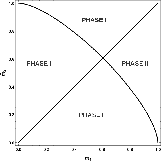
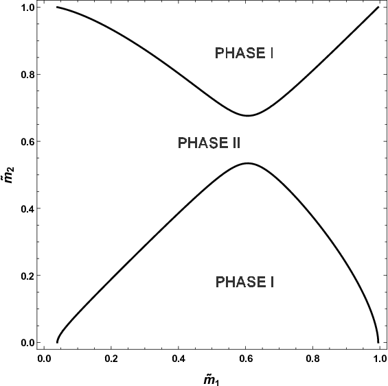
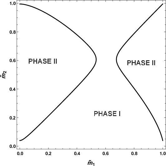
The phase space is illustrated in the figure (1) including the three cases : G2>G1G_{2}>G_{1} (right panel), G2=G1G_{2}=G_{1} (middle panel) and G1>G2G_{1}>G_{2} (right panel). We use G3≠0G_{3}\neq 0 in all plots. The masses (m~1,m~2)(\tilde{m}_{1},\tilde{m}_{2}) are normalized by the energy scale (μ)(\mu), i.e., m~i≡mi/μ⁡(i=1,2)\tilde{m}_{i}\equiv m_{i}/\mu\,(i=1,2).

Refer to caption
Refer to caption
Refer to caption
Figure 1: The phase diagram of the model for G3≠0G_{3}\neq 0, with the conditions G2>G1G_{2}>G_{1} (left panel), G1=G2G_{1}=G_{2} (middle panel) and G1>G2G_{1}>G_{2} (right panel), respectively. The phase I refers to the region in which βμ=0\beta^{\mu}=0 and αμ≠0\alpha^{\mu}\neq 0, while the phase II region correspond to αμ=0\alpha^{\mu}=0 and βμ≠0\beta^{\mu}\neq 0. The masses are normalized in energy scale unit.

It is important to highlight that only in the case g3=0g_{3}=0, both pseudo-vectors can acquire non-null vacuum expected values. Notice that, in both solutions, we have defined the renormalizable coupling constants

g1​R2g2=g12g2−m12π2​ϵ​and​g2​R2g′2=g22g′2−m22π2​ϵ.\displaystyle\frac{g_{1R}^{2}}{g^{2}}=\frac{g_{1}^{2}}{g^{2}}-\frac{m_{1}^{2}}{\pi^{2}\epsilon}\hskip 8.5359pt\mbox{and}\hskip 8.5359pt\frac{g_{2R}^{2}}{g^{\prime 2}}=\frac{g_{2}^{2}}{g^{\prime 2}}-\frac{m_{2}^{2}}{\pi^{2}\epsilon}\;. (33)

The true solution of the gap equation is defined by the global minimum of the potential. Integrating the gap equations, we obtain the effective potential:

Ve​f​f​(A,B)=g212​π2​(A2−a2)2+\displaystyle V_{eff}(A,B)=\frac{g^{2}}{12\pi^{2}}\left(A^{2}-a^{2}\right)^{2}+
+g′ 212​π2​(B2−b2)2−g32​A⋅B.\displaystyle+\,\frac{g^{\prime\,2}}{12\pi^{2}}\left(B^{2}-b^{2}\right)^{2}-g_{3}^{2}\,A\cdot B\;. (34)

Thereby, true minimum of the potential is at the points

a2\displaystyle a^{2}\!\! =\displaystyle= 3​π2​[g1​R2g2+m12π2​ln⁡(m1Λ)]​and​bμ=0,\displaystyle\!\!3\pi^{2}\left[\frac{g_{1R}^{2}}{g^{2}}+\frac{m_{1}^{2}}{\pi^{2}}\ln\left(\frac{m_{1}}{\Lambda}\right)\right]\hskip 4.26773pt\mbox{and}\hskip 4.26773ptb^{\mu}=0\;,
b2\displaystyle b^{2}\!\! =\displaystyle= 3​π2​[g2​R2g′2+m22π2​ln⁡(m2Λ)]​and​aμ=0.\displaystyle\!\!3\pi^{2}\left[\frac{g_{2R}^{2}}{g^{\prime 2}}+\frac{m_{2}^{2}}{\pi^{2}}\ln\left(\frac{m_{2}}{\Lambda}\right)\right]\hskip 4.26773pt\mbox{and}\hskip 4.26773pta^{\mu}=0\;.

If we consider a very small mass for ψ1\psi_{1}-majorana fermion, the first minimum point is determinate by the renormalized coupling constant g1​Rg_{1R}, i. e., a2=3​π2​g1​R2/g2a^{2}=3\pi^{2}g_{1R}^{2}/g^{2}. The effective potential has a nontrivial minimal in which ⟨Aμ⟩=αμ\langle A^{\mu}\rangle=\alpha^{\mu} and ⟨Bμ⟩=βμ\langle B^{\mu}\rangle=\beta^{\mu} are two scales of VEVs that break the Lorentz symmetry.

As consequence, the modified dispersion relations for the Majorana fermions are read below. In the phase I :

(p2−m12−a2)2+4​[p2​a2−(p⋅a)2]=0,\displaystyle(p^{2}-m_{1}^{2}-a^{2})^{2}+4\left[p^{2}\,a^{2}-(p\cdot a)^{2}\right]=0\;,\hskip 28.45274pt (36a)
p2=m22,\displaystyle p^{2}=m_{2}^{2}\;, (36b)

and in the phase II:

p2=m12,\displaystyle p^{2}=m_{1}^{2}\;,\penalty\ \penalty\ (37a)
(p2−m22−b2)2+4​[p2​b2−(p⋅b)2]=0.\displaystyle(p^{2}-m_{2}^{2}-b^{2})^{2}+4\left[p^{2}\,b^{2}-(p\cdot b)^{2}\right]=0\;.\hskip 28.45274pt (37b)

These dispersion relations are analogous to Carroll-Field-Jackiw-Proca electrodynamics [31]. The frequency solutions from (36a) and (37b) are hard to obtain in this present form. Thus, we can consider the particular cases of a time-like and space-like DLSB parameter. For a time-like case, in which aμ=(a0,𝟎)a^{\mu}=(a^{0},{\bf 0}) and bμ=(b0,𝟎)b^{\mu}=(b^{0},{\bf 0}), the frequency solutions are read below :

ω1(±)​(𝐩)\displaystyle\omega_{1}^{(\pm)}({\bf p})\!\! =\displaystyle= (|𝐩|±a0)2+m12\displaystyle\!\!\sqrt{(|{\bf p}|\pm a_{0})^{2}+m_{1}^{2}} (38)
≃\displaystyle\simeq ||𝐩|±a0|+m122​||𝐩|±a0|,\displaystyle\!\!||{\bf p}|\pm a_{0}|+\frac{m_{1}^{2}}{2||{\bf p}|\pm a_{0}|}\;,

and

ω2(±)​(𝐩)\displaystyle\omega_{2}^{(\pm)}({\bf p})\!\! =\displaystyle= (|𝐩|±b0)2+m22\displaystyle\!\!\sqrt{(|{\bf p}|\pm b_{0})^{2}+m_{2}^{2}} (39)
≃\displaystyle\simeq m2+(|𝐩|±b0)22​m2.\displaystyle\!\!m_{2}+\frac{(|{\bf p}|\pm b_{0})^{2}}{2m_{2}}\;.

For the space-like case, where aμ=(0,𝐚)a^{\mu}=(0,{\bf a}) and bμ=(0,𝐛)b^{\mu}=(0,{\bf b}), the frequency solutions are given by

ω1(±)​(𝐩)\displaystyle\omega_{1}^{(\pm)}({\bf p})\!\! =\displaystyle= 𝐩2+m12+𝐚2±2​|𝐚|​m12+(𝐩⋅𝐚^)2\displaystyle\!\!\sqrt{{\bf p}^{2}+m_{1}^{2}+{\bf a}^{2}\pm 2|{\bf a}|\sqrt{m_{1}^{2}+({\bf p}\cdot\hat{{\bf a}})^{2}}} (40)
≃\displaystyle\simeq |𝐩±𝐚|+m122​|𝐩±𝐚|,\displaystyle\!\!|{\bf p}\pm{\bf a}|+\frac{m_{1}^{2}}{2|{\bf p}\pm{\bf a}|}\;,

and

ω2(±)​(𝐩)\displaystyle\omega_{2}^{(\pm)}({\bf p})\!\! =\displaystyle= 𝐩2+m22+𝐛2±2​|𝐛|​m22+(𝐩⋅𝐛^)2\displaystyle\!\!\sqrt{{\bf p}^{2}+m_{2}^{2}+{\bf b}^{2}\pm 2|{\bf b}|\sqrt{m_{2}^{2}+({\bf p}\cdot\hat{{\bf b}})^{2}}} (41)
≃\displaystyle\simeq m2±|𝐛|+𝐩22​m2.\displaystyle\!\!m_{2}\pm|{\bf b}|+\frac{{\bf p}^{2}}{2m_{2}}\;.

We have considered the condition from the seesaw mechanism m2≫m1m_{2}\gg m_{1} in the previous approximation. For the massless case, for example, if we consider ψ1\psi_{1} a Majorana fermion with a very small mass in which we can neglect it m1≈0m_{1}\approx 0 with a generic DLSB parameter, the frequencies are given by

ω1±​(𝐩)\displaystyle\omega_{1}^{\pm}({\bf p})\!\! =\displaystyle= −a0±|𝐩+𝐚|,\displaystyle\!\!-a_{0}\,\pm\,|{\bf p}+{\bf a}|\;,\hskip 22.76228pt (42a)
ω2±​(𝐩)\displaystyle\omega_{2}^{\pm}({\bf p})\!\! =\displaystyle= a0±|𝐩−𝐚|.\displaystyle\!\!a_{0}\,\pm\,|{\bf p}-{\bf a}|\;.\hskip 22.76228pt (42b)

The usual RDs are recovered when aμ→0a^{\mu}\rightarrow 0. Other important point is that the results (42a) reproduce asymmetric frequencies and it depend on the direction of the vector 𝐚{\bf a} with a propagation direction 𝐩^\hat{{\bf p}}.

IV The effective action

The vacuum properties of the model help us to understand the dynamics of the fluctuations dictated by the auxiliary fields AμA^{\mu} and BμB^{\mu}. Thereby, we expand these auxiliary fields around the vacuum minimal as : Aμ​(x)=αμ+Xμ​(x)A^{\mu}(x)=\alpha^{\mu}+X^{\mu}(x) and Bμ​(x)=βμ+Yμ​(x)B^{\mu}(x)=\beta^{\mu}+Y^{\mu}(x), respectively, where XμX^{\mu} and YμY^{\mu} are interpreted as the new dynamical fields of the model, and {αμ,βμ}\left\{\,\alpha^{\mu}\,,\,\beta^{\mu}\,\right\} do not depend on the space-time coordinates. The effective action in terms of XμX^{\mu} and YμY^{\mu} is

Se​f​f(X,Y)=∫d4x{12g12α2+12g22β2\displaystyle S_{eff}(X,Y)=\!\!\int d^{4}x\,\Bigg\{\frac{1}{2}\,g_{1}^{2}\,\alpha^{2}+\frac{1}{2}\,g_{2}^{2}\,\beta^{2}
+g32​(α⋅β)+X⋅(g12​α+g32​β)+Y⋅(g22​β+g32​α)\displaystyle+g_{3}^{2}\,(\alpha\cdot\beta)+X\cdot(g_{1}^{2}\alpha+g_{3}^{2}\beta)+Y\cdot(g_{2}^{2}\beta+g_{3}^{2}\alpha)
+12​g12​X2+12​g22​Y2+g32​(X⋅Y)\displaystyle+\frac{1}{2}\,g_{1}^{2}\,X^{2}+\frac{1}{2}\,g_{2}^{2}\,Y^{2}+g_{3}^{2}\,(X\cdot Y)
−i∫d4​p(2​π)4tr[ln(/p−m1−/aγ5−g/Xγ5)]\displaystyle-i\!\int\frac{d^{4}p}{(2\pi)^{4}}\,\mbox{tr}\left[\ln\left(\,/\penalty{\!\!\!p}-m_{1}-/\penalty{\!\!\!a}\,\gamma_{5}-g\,\,/\penalty{\!\!\!\!X}\,\gamma_{5}\,\right)\right]
−i∫d4​p(2​π)4tr[ln(/p−m2−/bγ5−g′/Yγ5)]}.\displaystyle-i\!\int\frac{d^{4}p}{(2\pi)^{4}}\,\mbox{tr}\left[\ln\left(\,/\penalty{\!\!\!p}-m_{2}-/\penalty{\!\!\!b}\,\gamma_{5}-g^{\prime}\,/\penalty{\!\!\!Y}\,\gamma_{5}\,\right)\right]\Bigg\}.

Now, we expand the previous effective action in power series of XμX^{\mu} and YμY^{\mu}, such that:

Se​f​f​(X,Y)=∑n=1∞S(n)​(X,Y),\displaystyle S_{eff}(X,Y)=\sum_{n=1}^{\infty}S^{(n)}(X,Y)\;, (44)

where the first correction (n=1)(n=1) is given by

S(1)​(X,Y)\displaystyle S^{(1)}(X,Y)\!\! =\displaystyle= i∫d4x[Xμ(iΠ1μ−g12αμ−g32βμ)+\displaystyle\!\!i\int d^{4}x\Big[\,X_{\mu}\left(i\Pi_{1}^{\mu}-g_{1}^{2}\,\alpha^{\mu}-g_{3}^{2}\,\beta^{\mu}\right)+ (45)
+Yμ(iΠ2μ−g22βμ−g32αμ)]=0.\displaystyle\hskip-34.14322pt+Y_{\mu}\left(i\Pi_{2}^{\mu}-g_{2}^{2}\,\beta^{\mu}-g_{3}^{2}\,\alpha^{\mu}\right)\,\Big]=0\;.

This contribution is null, as we expect, due to the relations (25a) and (25b). The self-energy term is the correction at the second order :

S(2)​(X,Y)=i2​∑i,j=12∫d4​x​[Vμi​(x)​Πi​jμ​ν​Vνj​(x)],\displaystyle S^{(2)}(X,Y)=\frac{i}{2}\sum_{i,j=1}^{2}\int d^{4}x\Big[\,V_{\mu}^{i}(x)\,\Pi^{\mu\nu}_{ij}\,V_{\nu}^{j}(x)\,\Big]\,,\hskip 8.5359pt (46)

where we have introduced the notation Vμi=(Vμ1,Vμ2)≡(Xμ,Yμ)V_{\mu}^{i}=(\,V_{\mu}^{1}\,,\,V_{\mu}^{2}\,)\equiv(\,X_{\mu}\,,\,Y_{\mu}\,), and the vacuum polarizations are given by

Π11μ​ν=−i​ημ​ν​g12+\displaystyle\Pi^{\mu\nu}_{11}=-i\,\eta^{\mu\nu}\,g_{1}^{2}+
+Tr​[(−i​g​γμ​γ5)​S1​(p)​(−i​g​γν​γ5)​S1​(p−k)],\displaystyle\hskip-22.76228pt+\mbox{Tr}\Big[(-ig\gamma^{\mu}\gamma_{5})S_{1}(p)(-ig\gamma^{\nu}\gamma_{5})S_{1}(p-k)\Big],\;\;\; (47a)
Π12μ​ν=Π21μ​ν=−i​ημ​ν​g32,\displaystyle\Pi^{\mu\nu}_{12}=\Pi^{\mu\nu}_{21}=-i\,\eta^{\mu\nu}\,g_{3}^{2}\;, (47b)
Π22μ​ν=−i​ημ​ν​g22+\displaystyle\Pi^{\mu\nu}_{22}=-i\,\eta^{\mu\nu}\,g_{2}^{2}+
+Tr​[(−i​g′​γμ​γ5)​S2​(p)​(−i​g′​γν​γ5)​S2​(p−k)],\displaystyle\hskip-22.76228pt+\mbox{Tr}\Big[(-ig^{\prime}\gamma^{\mu}\gamma_{5})S_{2}(p)(-ig^{\prime}\gamma^{\nu}\gamma_{5})S_{2}(p-k)\Big],\;\;\; (47c)

in which

S1​(p)=ip̸−m1−a̸​γ5,\displaystyle S_{1}(p)=\frac{i}{\not{p}-m_{1}-\not{a}\,\gamma_{5}}\;, (48a)
S2​(p)=ip̸−m2−b̸​γ5.\displaystyle S_{2}(p)=\frac{i}{\not{p}-m_{2}-\not{b}\,\gamma_{5}}\;. (48b)

Since we know that m2≫m1m_{2}\gg m_{1} through the seesaw mechanism, we fix the ψ2\psi_{2} mass at the energy scale (Λ)(\Lambda), i.e., m2∼Λm_{2}\sim\Lambda. In this case, the gap equations (30) and (30) are simplified to a2≈3​π2​g1​R2/g2a^{2}\approx 3\pi^{2}g_{1R}^{2}/g^{2}, when bμ=0b^{\mu}=0, and b2≈3​π2​g2​R2/g′2b^{2}\approx 3\pi^{2}g_{2R}^{2}/g^{\prime 2} , when aμ=0a^{\mu}=0, respectively. The global minima is defined for the condition g1​R>g2​Rg_{1R}>g_{2R} in the first gap, and g2​R>g1​Rg_{2R}>g_{1R} in the second gap. Since experimental measurements point out to a null or very small value for |a2||a^{2}| which couples with the SM neutrino, we can consider the condition g2​R>g1​Rg_{2R}>g_{1R}. Under these conditions, we obtain the vacuum polarizations in the position space

Π11μ​ν\displaystyle\Pi^{\mu\nu}_{11} =\displaystyle= −i​ημ​ν​{g12−g2​m122​π2​[1ϵ−2​ln⁡(m1Λ)]}\displaystyle-i\,\eta^{\mu\nu}\left\{g_{1}^{2}-\frac{g^{2}m_{1}^{2}}{2\pi^{2}}\left[\frac{1}{\epsilon}-2\ln\Big(\frac{m_{1}}{\Lambda}\Big)\right]\right\} (49a)
−i​g212​π2[1−1ϵ+2ln(m1Λ)](ημ​ν□−∂μ∂ν)−i​g212​π2∂μ∂ν,\displaystyle-\frac{ig^{2}}{12\pi^{2}}\!\Big[1-\frac{1}{\epsilon}+2\ln\Big(\frac{m_{1}}{\Lambda}\Big)\Big]\left(\eta^{\mu\nu}\Box-\partial^{\mu}\partial^{\nu}\right)-\frac{ig^{2}}{12\pi^{2}}\,\partial^{\mu}\partial^{\nu}\,,
Π22μ​ν\displaystyle\Pi^{\mu\nu}_{22} =\displaystyle= −i​ημ​ν​{g22−g′2​b2π2−g′2​m222​π2​[1ϵ−2​ln⁡(m2Λ)]}\displaystyle-i\,\eta^{\mu\nu}\!\left\{g_{2}^{2}-\frac{g^{\prime 2}b^{2}}{\pi^{2}}-\frac{g^{\prime 2}m_{2}^{2}}{2\pi^{2}}\left[\frac{1}{\epsilon}-2\ln\Big(\frac{m_{2}}{\Lambda}\Big)\right]\right\} (49b)
−i​g′ 212​π2[1−1ϵ+2ln(m2Λ)](ημ​ν□−∂μ∂ν)−i​g′212​π2∂μ∂ν\displaystyle-\frac{ig^{\prime\,2}}{12\pi^{2}}\left[1-\frac{1}{\epsilon}+2\ln\Big(\frac{m_{2}}{\Lambda}\Big)\right](\eta^{\mu\nu}\Box-\partial^{\mu}\partial^{\nu})-\frac{ig^{\prime 2}}{12\pi^{2}}\,\partial^{\mu}\partial^{\nu}
+i​g′212​π2(bμ∂ν−bν∂μ)−i​g′ 24​π2[1ϵ−2ln(m2Λ)]ϵμ​ν​ρ​σbρ∂σ\displaystyle+\frac{ig^{\prime 2}}{12\pi^{2}}\left(b^{\mu}\partial^{\nu}-b^{\nu}\partial^{\mu}\right)-\frac{ig^{\prime\,2}}{4\pi^{2}}\left[\frac{1}{\epsilon}-2\ln\Big(\frac{m_{2}}{\Lambda}\Big)\right]\epsilon^{\mu\nu\rho\sigma}b_{\rho}\partial_{\sigma}
+g′24​π2​{1−92​[1ϵ−2​ln⁡(m2Λ)]}​bμ​bν.\displaystyle+\frac{g^{\prime 2}}{4\pi^{2}}\left\{1-\frac{9}{2}\left[\frac{1}{\epsilon}-2\ln\left(\frac{m_{2}}{\Lambda}\right)\right]\right\}\,b^{\mu}\,b^{\nu}\,.

Substituting these results in (46), we write the effective action as

Se​f​f(2)=∫d4​x​ℒe​f​f(2),\displaystyle S_{eff}^{(2)}=\int d^{4}x\,{\cal L}_{eff}^{(2)}\;, (50)

where the renormalizable effective lagrangian (at the second order) is given by

ℒe​f​f(2)=−14​XR​μ​ν2−gR224​π2​(∂μXRμ)2+12​(6​m12)​XR​μ2\displaystyle{\cal L}_{eff}^{(2)}=-\frac{1}{4}X_{R\mu\nu}^{2}\!-\!\frac{g_{R}^{2}}{24\pi^{2}}\,(\partial_{\mu}X_{R}^{\,\,\mu})^{2}\!+\!\frac{1}{2}(6m_{1}^{2})X_{R\mu}^{2}
−14​YR​μ​ν2−gR′ 224​π2​(∂μYRμ)2+12​(6​m22)​YR​μ2\displaystyle-\frac{1}{4}\,Y_{R\mu\nu}^{2}-\frac{g_{R}^{\prime\,2}}{24\pi^{2}}\,(\partial_{\mu}Y_{R}^{\,\,\mu})^{2}\!+\!\frac{1}{2}(6m_{2}^{2})Y_{R\mu}^{2}
+g3​R2​XR​μ​YRμ−gR′ 212​π2​(b⋅YR)​∂μYRμ\displaystyle+g_{3R}^{2}\,X_{R\mu}Y_{R}^{\,\,\mu}-\frac{g_{R}^{\prime\,2}}{12\pi^{2}}\,(b\cdot Y_{R})\,\partial_{\mu}Y_{R}^{\,\,\mu}
−274​(b⋅YR)2+34​bμ​ϵμ​ν​ρ​σ​YR​ν​YR​ρ​σ.\displaystyle-\frac{27}{4}\,(b\cdot Y_{R})^{2}+\frac{3}{4}\,b_{\mu}\,\epsilon^{\mu\nu\rho\sigma}Y_{R\nu}Y_{R\rho\sigma}\;. (51)

To get the effective lagrangian in this form, we have defined the renormalized fields

XRμ=Z3−1/2Xμ,YRμ=Z4−1/2Yμ,\displaystyle X_{R}^{\,\,\mu}=Z_{3}^{-1/2}X^{\mu}\;\;,\;\;Y_{R}^{\,\,\mu}=Z_{4}^{-1/2}Y^{\mu}\;, (52)

where the renormalization factors are given by

Z3−1\displaystyle Z_{3}^{-1}\!\! =\displaystyle= g212​π2​[1−1ϵ+2​ln⁡(m1Λ)],\displaystyle\!\!\frac{g^{2}}{12\pi^{2}}\left[1-\frac{1}{\epsilon}+2\,\ln\left(\frac{m_{1}}{\Lambda}\right)\right]\,, (53a)
Z4−1\displaystyle Z_{4}^{-1}\!\! =\displaystyle= g′ 212​π2​[1−1ϵ+2​ln⁡(m2Λ)],\displaystyle\!\!\frac{g^{\prime\,2}}{12\pi^{2}}\left[1-\frac{1}{\epsilon}+2\,\ln\left(\frac{m_{2}}{\Lambda}\right)\right]\,, (53b)

and the renormalized coupling constants are

gR=Z3​g,gR′=Z4​g′,g3​R=Z3​Z44​g3.\displaystyle g_{R}\!=\!\sqrt{Z_{3}}\,g\;,\;g_{R}^{\prime}\!=\!\sqrt{Z_{4}}\,g^{\prime}\;,\;g_{3R}\!=\!\sqrt[4]{Z_{3}Z_{4}}\,g_{3}\,.\;\; (54)

The transversal operators from (49a) and (49b) induces dynamical for the auxiliary vector fields through the field strength tensors Xμ​ν=∂μXν−∂νXμX_{\mu\nu}=\partial_{\mu}X_{\nu}-\partial_{\nu}X_{\mu} and Yμ​ν=∂μYν−∂νYμY_{\mu\nu}=\partial_{\mu}Y_{\nu}-\partial_{\nu}Y_{\mu}, respectively. In (IV), the correspondent renormalized field strength tensors are XR​μ​ν=Z3−1/2Xμ​νX_{R\mu\nu}=Z_{3}^{-1/2}X_{\mu\nu}, and YR​μ​ν=Z4−1/2Yμ​νY_{R\mu\nu}=Z_{4}^{-1/2}Y_{\mu\nu}. Furthermore, in (IV), the radiative corrections also induce a new Chern-Symons term depending on the bμb^{\mu}-parameter, YRμY_{R}^{\mu} and the field strength tensor YRμ​νY_{R}^{\mu\nu}. Note that, the effective lagrangian also shows quadratic terms in XRμX_{R}^{\mu} and YRμY_{R}^{\mu}, and also a mixed term of XRμX_{R}^{\mu} with YRμY_{R}^{\mu}. These terms are interpreted as like-massive terms of the auxiliary fields XRX_{R} and YRY_{R}. We can write these terms into the matrix form

ℒm​a​s​s−X​Y(2)=12​ημ​ν​(VR​μ)t​M2​VR​ν,\displaystyle{\cal L}_{mass-XY}^{(2)}=\frac{1}{2}\,\eta^{\mu\nu}(V_{R\mu})^{t}\,M^{2}\,V_{R\nu}\;, (55)

in which M2M^{2} is the mass matrix

M2=[6​m12g3​R2g3​R26​m22],\displaystyle M^{2}=\left[\begin{array}[]{cc}6m_{1}^{2}&g_{3R}^{2}\\ \\ g_{3R}^{2}&6m_{2}^{2}\\ \end{array}\right]\;,

and VRμV_{R}^{\mu} is the column vector formed by the fields XRμX_{R}^{\mu} and YRμY_{R}^{\mu}. This mass matrix can be diagonalized by a S​O​(2)SO(2) matrix, say ℛ{\cal R}, in which transformations in the vector fields are :

XRμ\displaystyle X_{R}^{\mu}\! =\displaystyle= cos⁡α​Z1​Rμ+sin⁡α​Z2​Rμ,\displaystyle\!\cos\alpha\,Z_{1R}^{\mu}+\sin\alpha\,Z_{2R}^{\mu}\,, (60a)
YRμ\displaystyle Y_{R}^{\mu}\! =\displaystyle= −sin⁡α​Z1​Rμ+cos⁡α​Z2​Rμ,\displaystyle\!-\sin\alpha\,Z_{1R}^{\mu}+\cos\alpha\,Z_{2R}^{\mu}\,, (60b)

where α\alpha is a mixing angle, such that, tan⁡(2​α)=g3​R2/(3​m22−3​m12)\tan(2\alpha)=g_{3R}^{2}/(3m_{2}^{2}-3m_{1}^{2}). The Z1​RμZ_{1R}^{\mu} and Z2​RμZ_{2R}^{\mu} are interpreted as the physical eigenstates for the auxiliary fields whose the masses are determinate by the diagonal matrix MD2=ℛt​M2​ℛ=diag​(μ12,μ22)M_{D}^{2}={\cal R}^{t}\,M^{2}\,{\cal R}=\mbox{diag}(\,\mu_{1}^{2}\,,\,\mu_{2}^{2}\,), in which the eigenvalues {μ12,μ22}\left\{\,\mu_{1}^{2}\,,\,\mu_{2}^{2}\,\right\} are, respectively, read below

μ12\displaystyle\mu_{1}^{2}\!\! =\displaystyle= 3​(m12+m22)−9​(m12−m22)2+g3​R4\displaystyle\!\!3\left(m_{1}^{2}+m_{2}^{2}\right)-\sqrt{9\left(m_{1}^{2}-m_{2}^{2}\right)^{2}+g_{3R}^{4}} (61a)
≃6​m12−g3​R46​m22,\displaystyle\simeq 6m_{1}^{2}-\frac{g_{3R}^{4}}{6m_{2}^{2}}\,,\hskip 14.22636pt
μ22\displaystyle\mu_{2}^{2}\!\! =\displaystyle= 3​(m12+m22)+9​(m12−m22)2+g3​R4\displaystyle\!\!3\left(m_{1}^{2}+m_{2}^{2}\right)+\sqrt{9\left(m_{1}^{2}-m_{2}^{2}\right)^{2}+g_{3R}^{4}} (61b)
≃6​m22+g3​R46​m22,\displaystyle\simeq 6m_{2}^{2}+\frac{g_{3R}^{4}}{6m_{2}^{2}}\,,\hskip 14.22636pt

in which we have used the condition m2≫m1m_{2}\gg m_{1}. Since that m2≫g3​Rm_{2}\gg g_{3R}, we identify μ1≃6​m1\mu_{1}\simeq\sqrt{6}\,m_{1} as the Z1​RZ_{1R} mass eigenstate (light gauge boson), while that μ2≃6​m2\mu_{2}\simeq\sqrt{6}\,m_{2} is the correspondent eigenstate for Z2​RZ_{2R} (heavy gauge boson). Under this condition, we can consider tan⁡(2​α)≃g3​R2/(3​m22)≪1\tan(2\alpha)\simeq g_{3R}^{2}/(3m_{2}^{2})\ll 1, such that sin⁡α≃g3​R2/(6​m22)≃0\sin\alpha\simeq g_{3R}^{2}/(6m_{2}^{2})\simeq 0 and cos⁡α≃1\cos\alpha\simeq 1. In the {Z1​R,Z2​R}\left\{\,Z_{1R}\,,\,Z_{2R}\,\right\} basis, the effective lagrangian (IV) is

ℒe​f​f(2)=−14​Z1​R​μ​ν2+12​μ12​Z1​R​μ2−gR224​π2​(∂μZ1​Rμ)2\displaystyle{\cal L}_{eff}^{(2)}=-\frac{1}{4}Z_{1R\mu\nu}^{2}+\frac{1}{2}\,\mu_{1}^{2}\,Z_{1R\mu}^{2}\!-\!\frac{g_{R}^{2}}{24\pi^{2}}\,(\partial_{\mu}Z_{1R}^{\,\,\mu})^{2}
−14​Z2​R​μ​ν2+12​μ22​Z2​R​μ2−gR′ 224​π2​(∂μZ2​Rμ)2\displaystyle-\frac{1}{4}\,Z_{2R\mu\nu}^{2}+\frac{1}{2}\,\mu_{2}^{2}\,Z_{2R\mu}^{2}-\frac{g_{R}^{\prime\,2}}{24\pi^{2}}\,(\partial_{\mu}Z_{2R}^{\,\,\mu})^{2}
−gR′ 212​π2(b⋅Z2​R)∂μZ2​Rμ−274(b⋅Z2​R)2\displaystyle-\frac{g_{R}^{\prime\,2}}{12\pi^{2}}\,(b\cdot Z_{2R})\,\partial_{\mu}Z_{2R}^{\,\,\mu}-\frac{27}{4}\,(b\cdot Z_{2R})^{2}
+34​bμ​ϵμ​ν​ρ​σ​Z2​R​ν​Z2​R​ρ​σ.\displaystyle+\frac{3}{4}\,b_{\mu}\,\epsilon^{\mu\nu\rho\sigma}\,Z_{2R\nu}\,Z_{2R\rho\sigma}\,. (62)

Notice that the Chern-Symons term emerges for the Z2​RμZ_{2R}^{\,\,\mu} physical eigenstate when the mixing with the Z1​RμZ_{1R}^{\,\,\mu} is very weak. The action principle yields the field equations :

∂μZ1​Rμ​ν+μ12​Z1​Rν+gR212​π2​∂ν(∂μZ1​Rμ)=0,\displaystyle\partial_{\mu}Z_{1R}^{\mu\nu}+\mu_{1}^{2}\,Z_{1R}^{\nu}\!+\!\frac{g_{R}^{2}}{12\pi^{2}}\,\partial^{\nu}(\partial_{\mu}Z_{1R}^{\,\,\mu})=0\,,\hskip 14.22636pt (63a)
∂μZ2​Rμ​ν+μ22​Z2​Rν+gR′ 212​π2​∂ν(∂μZ2​Rμ)\displaystyle\partial_{\mu}Z_{2R}^{\mu\nu}+\mu_{2}^{2}\,Z_{2R}^{\nu}\!+\!\frac{g_{R}^{\prime\,2}}{12\pi^{2}}\,\partial^{\nu}(\partial_{\mu}Z_{2R}^{\,\,\mu})
−gR′ 212​π2​[bν​∂μZ2​Rμ−∂ν(b⋅Z2​R)]\displaystyle-\frac{g_{R}^{\prime\,2}}{12\pi^{2}}\left[\,b^{\nu}\,\partial_{\mu}Z_{2R}^{\,\,\mu}-\partial^{\nu}(b\cdot Z_{2R})\right]
+32​ϵμ​ν​ρ​σ​bμ​Z2​R​ρ​σ=0.\displaystyle+\frac{3}{2}\,\epsilon^{\mu\nu\rho\sigma}\,b_{\mu}\,Z_{2R\rho\sigma}=0\,. (63b)

Operating ∂ν\partial_{\nu} on the equations (63a) and (63b), the longitudinal part of Z1​RZ_{1R} and Z2​RZ_{2R} satisfies the relations

(□+12​π2​μ12gR2)​∂μZ1​Rμ=0,\displaystyle\left(\Box+\frac{12\pi^{2}\mu_{1}^{2}}{g_{R}^{2}}\right)\partial_{\mu}Z_{1R}^{\mu}=0\;, (64a)
(□−b⋅∂+12​π2​μ22gR2′)∂μZ2​Rμ+□(b⋅Z2​R)=0.\displaystyle\left(\Box-b\cdot\partial+\frac{12\pi^{2}\mu_{2}^{2}}{g_{R}^{2\,\prime}}\right)\partial_{\mu}Z_{2R}^{\mu}+\Box(b\cdot Z_{2R})=0\;.

Substituting the plane wave solutions Zi​Rμ​(x)=zi​Rμ​ei​k⋅x​(i=1,2)Z_{iR}^{\mu}(x)=z_{iR}^{\mu}\,e^{ik\cdot x}\,(i=1,2), in which zi​Rμz_{iR}^{\mu} are the constant and uniform wave amplitudes, the equations (63a) and (63b) can be written as M1μ​ν​z1​R​μ=0M_{1}^{\mu\nu}\,z_{1R\mu}=0 and M2μ​ν​z2​R​μ=0M_{2}^{\mu\nu}\,z_{2R\mu}=0, respectively, where the matrices Miμ​ν​(i=1,2)M_{i}^{\mu\nu}\,(i=1,2) are given by

M1μ​ν\displaystyle M_{1}^{\mu\nu}\!\! =\displaystyle= (−k2+μ12)​ημ​ν+(1−gR212​π2)​kμ​kν,\displaystyle\!\!\left(-k^{2}+\mu_{1}^{2}\right)\eta^{\mu\nu}+\left(1-\frac{g_{R}^{2}}{12\pi^{2}}\right)k^{\mu}k^{\nu}\;,\hskip 22.76228pt (65a)
M2μ​ν\displaystyle M_{2}^{\mu\nu}\!\! =\displaystyle= (−k2+μ22)​ημ​ν+(1−gR′ 212​π2)​kμ​kν\displaystyle\!\!\left(-k^{2}+\mu_{2}^{2}\right)\eta^{\mu\nu}+\left(1-\frac{g_{R}^{\prime\,2}}{12\pi^{2}}\right)k^{\mu}k^{\nu} (65b)
+i​gR′ 212​π2​(bμ​kν−bν​kμ)+i​ 3​ϵμ​ν​ρ​σ​bρ​kσ.\displaystyle\hskip-14.22636pt+\frac{ig_{R}^{\prime\,2}}{12\pi^{2}}\left(b^{\mu}k^{\nu}-b^{\nu}k^{\mu}\right)+i\,3\,\epsilon^{\mu\nu\rho\sigma}\,b_{\rho}\,k_{\sigma}\;.

The dispersion relations are determinate by the conditions det​(M1μ​ν)=0\mbox{det}(M_{1}^{\mu\nu})=0 and det​(M2μ​ν)=0\mbox{det}(M_{2}^{\mu\nu})=0. The null determinant of M1μ​νM_{1}^{\mu\nu} yields the frequencies solutions ωZ1​R(i)±=±ωZ1​R(i)​(𝐤)​(i=1,2)\omega_{Z_{1R}}^{(i)\pm}=\pm\,\omega_{Z_{1R}}^{(i)}({\bf k})\,(i=1,2), in which the dispersion relations ωZ1​R(i)​(𝐤)\omega_{Z_{1R}}^{(i)}({\bf k}) are read below :

ωZ1​R(1)​(𝐤)\displaystyle\omega_{Z_{1R}}^{(1)}({\bf k})\! =\displaystyle= 𝐤2+μ12,\displaystyle\!\sqrt{{\bf k}^{2}+\mu_{1}^{2}}\;, (66a)
ωZ1​R(2)​(𝐤)\displaystyle\omega_{Z_{1R}}^{(2)}({\bf k})\! =\displaystyle= 𝐤2+12​π2​μ12gR2.\displaystyle\!\sqrt{{\bf k}^{2}+\frac{12\pi^{2}\mu_{1}^{2}}{g_{R}^{2}}}\;. (66b)

The frequency (66a) is the transversal mode of Z1​RZ_{1R} with mass μ1=6​m1\mu_{1}=\sqrt{6}\,m_{1}, and (66b) is the frequency associated with longitudinal propagation mode of Z1​RZ_{1R}. For the case of M2μ​νM_{2}^{\mu\nu}, we assume a time-like vector bμ=(b0,𝟎)b^{\mu}=(b_{0},{\bf 0}) in which four roots are possible for the null determinant : ωZ2​R(i)±=±ωZ2​R(i)​(𝐤)​(i=1,2,3,4)\omega_{Z_{2R}}^{(i)\pm}=\pm\,\omega_{Z_{2R}}^{(i)}({\bf k})\,(i=1,2,3,4). These frequencies are given by

ωZ2​R(1)​(𝐤)\displaystyle\omega_{Z_{2R}}^{(1)}({\bf k})\!\! =\displaystyle= 𝐤2−3​|b0|​|𝐤|+μ22,\displaystyle\!\!\sqrt{{\bf k}^{2}-3|b_{0}||{\bf k}|+\mu_{2}^{2}}\;, (67a)
ωZ2​R(2)​(𝐤)\displaystyle\omega_{Z_{2R}}^{(2)}({\bf k})\!\! =\displaystyle= 𝐤2+3​|b0|​|𝐤|+μ22,\displaystyle\!\!\sqrt{{\bf k}^{2}+3|b_{0}||{\bf k}|+\mu_{2}^{2}}\;, (67b)
ωZ2​R(3)​(𝐤)\displaystyle\omega_{Z_{2R}}^{(3)}({\bf k})\!\! =\displaystyle= 𝐤2+3​π​(gR′ 2+12​π2)​μ22−9​π2​(gR′ 2−12​π2)2​μ24−3​b02​gR′ 6​𝐤26​π​gR′ 2,\displaystyle\!\!\sqrt{{\bf k}^{2}+\frac{3\pi(g_{R}^{\prime\,2}+12\pi^{2})\mu_{2}^{2}-\sqrt{9\pi^{2}(g_{R}^{\prime\,2}-12\pi^{2})^{2}\mu_{2}^{4}-3b_{0}^{2}\,g_{R}^{\prime\,6}\,{\bf k}^{2}}}{6\pi g_{R}^{\prime\,2}}}\;, (67c)
ωZ2​R(4)​(𝐤)\displaystyle\omega_{Z_{2R}}^{(4)}({\bf k})\!\! =\displaystyle= 𝐤2+3​π​(gR′ 2+12​π2)​μ22+9​π2​(gR′ 2−12​π2)2​μ24−3​b02​gR′ 6​𝐤26​π​gR′ 2.\displaystyle\!\!\sqrt{{\bf k}^{2}+\frac{3\pi(g_{R}^{\prime\,2}+12\pi^{2})\mu_{2}^{2}+\sqrt{9\pi^{2}(g_{R}^{\prime\,2}-12\pi^{2})^{2}\mu_{2}^{4}-3b_{0}^{2}\,g_{R}^{\prime\,6}\,{\bf k}^{2}}}{6\pi g_{R}^{\prime\,2}}}\;. (67d)

Notice that, when b0→0b_{0}\rightarrow 0, the previous frequencies reduce to (66a) and (66b)(\ref{omega2Z1R}) exchanging gR′→gRg_{R}^{\prime}\rightarrow g_{R} and μ2→μ1\mu_{2}\rightarrow\mu_{1}.

Finally, we obtain the n=3n=3 contribution to the effective action, under the condition aμ=0a^{\mu}=0 and bμ≠0b^{\mu}\neq 0, is :

Πμ​ν​ρX\displaystyle\Pi^{X}_{\;\;\mu\nu\rho}\!\! =\displaystyle= 0,\displaystyle\!\!0\;, (68a)
Πμ​ν​ρY\displaystyle\Pi^{Y}_{\;\;\mu\nu\rho}\!\! =\displaystyle= i​g′ 33​π2​(βμ​ην​ρ+βν​ην​ρ+βρ​ημ​ν).\displaystyle\!\!\frac{ig^{\prime\,3}}{3\pi^{2}}\left(\beta_{\mu}\,\eta_{\nu\rho}+\beta_{\nu}\,\eta_{\nu\rho}+\beta_{\rho}\,\eta_{\mu\nu}\right).\;\; (68b)

The divergent contribution vanishes due to the index symmetry. For the n=4n=4 contribution, one finds:

Πμ​ν​ρ​κX\displaystyle\Pi^{X}_{\;\;\mu\nu\rho\kappa}\!\! =\displaystyle= i​g43​π2​(ημ​ν​ηρ​κ−ημ​ρ​ην​κ+ημ​κ​ην​ρ),\displaystyle\!\!\frac{ig^{4}}{3\pi^{2}}\left(\eta_{\mu\nu}\eta_{\rho\kappa}-\eta_{\mu\rho}\eta_{\nu\kappa}+\eta_{\mu\kappa}\eta_{\nu\rho}\right),\hskip 22.76228pt (69a)
Πμ​ν​ρ​κY\displaystyle\Pi^{Y}_{\;\;\mu\nu\rho\kappa}\!\! =\displaystyle= i​g′ 43​π2​(ημ​ν​ηρ​κ−ημ​ρ​ην​κ+ημ​κ​ην​ρ).\displaystyle\!\!\frac{ig^{\prime\,4}}{3\pi^{2}}\left(\eta_{\mu\nu}\eta_{\rho\kappa}-\eta_{\mu\rho}\eta_{\nu\kappa}+\eta_{\mu\kappa}\eta_{\nu\rho}\right).\hskip 22.76228pt (69b)

Again, the divergence vanishes due to the index symmetry. Therefore, using these results, the renormalized effective potential can be written in terms of the physical eigenstates {Z1​R,Z2​R}\{\,Z_{1R}\,,\,Z_{2R}\,\} as :

Ve​f​f​(Z1​R,Z2​R)=−12​μ12​Z1​R2+gR412​π2​(Z1​R2)2\displaystyle V_{eff}(Z_{1R},Z_{2R})=-\frac{1}{2}\,\mu_{1}^{2}\,Z_{1R}^{2}+\frac{g_{R}^{4}}{12\pi^{2}}\left(Z_{1R}^{2}\right)^{2}
−12​μ22​Z2​R2+(gR′)412​π2​(Z2​R2+2gR′​Z2​R⋅b)2.\displaystyle-\frac{1}{2}\,\mu_{2}^{2}\,Z_{2R}^{2}+\frac{(g^{\prime}_{R})^{4}}{12\pi^{2}}\left(Z_{2R}^{2}+\frac{2}{g^{\prime}_{R}}Z_{2R}\cdot b\right)^{2}\!\!.\,\, (70)

where we have fixed the condition aμ=0a^{\mu}=0, with the shift Bμ→bμgR′+YμB^{\mu}\rightarrow\frac{b^{\mu}}{g^{\prime}_{R}}+Y^{\mu}, and the rotation to the physical eigenstates from (60a) and (60b).

V Neutrino Oscillations in the DLSB scenario

Since the discovery of the oscillation phenomena associated with the non-null neutrino’s masses in a basis which does not match with the flavor basis of the SM, several models beyond the SM were proposed in order to explain this phenomena in the literature [32, 33, 34]. We start the description of the oscillation phenomena considering the three flavor neutrinos eigenstates |να⟩={|νe⟩,|νμ⟩,|μτ⟩}|\nu_{\alpha}\rangle=\left\{\,|\nu_{e}\rangle\,,\,|\nu_{\mu}\rangle\,,\,|\mu_{\tau}\rangle\,\right\}. After the seesaw mechanism takes place, we define the physical eigenstates |νi⟩|\nu_{i}\rangle, with i={ 1, 2, 3}i=\left\{\,1,\,2\,,\,3\,\right\}, that represent the LHNs with light masses. These physical eigenstates are related with the previous flavour neutrinos eigenstates by the transformation

|νi⟩=∑αUi​α​|να⟩,|να⟩=∑iUα​i∗​|νi⟩,|\nu_{i}\rangle=\sum_{\alpha}U_{i\alpha}\,|\nu_{\alpha}\rangle\penalty\ \penalty\ \penalty\ ,\penalty\ \penalty\ \penalty\ |\nu_{\alpha}\rangle=\sum_{i}U^{\ast}_{\alpha i}\,|\nu_{i}\rangle\;, (71)

in which Ui​αU_{i\alpha} is the so-called Pontecorvo–Maki–Nakagawa–Sakata (PMNS) unitary and complex matrix. The dynamic of the physical eigenstates is ruled by the spatial-time evolution:

|νi​(𝐱,t)⟩=ei⁡(Ei​t+𝐩i⋅𝐱)​|νi​(0,0)⟩.|\nu_{i}({\bf x},t)\rangle=e^{i(E_{i}t+{\bf p}_{i}\cdot{\bf x})}\,|\nu_{i}(0,0)\rangle\;. (72)

Therefore, the transition probability of oscillation between flavors states |να⟩→|νβ⟩|\nu_{\alpha}\rangle\rightarrow|\nu_{\beta}\rangle is defined by

Pα→β​(𝐱,t)=|⟨να​(𝐱,t)|νβ​(𝐱,t)⟩|2\displaystyle P_{\alpha\rightarrow\beta}({\bf x},t)=|\langle\nu_{\alpha}({\bf x},t)|\nu_{\beta}({\bf x},t)\rangle|^{2}
=|∑iUi​α∗​Ui​β​ei​Ei​t​ei​𝐩i⋅𝐱|2.\displaystyle=\Bigg|\sum_{i}U^{\ast}_{i\alpha}\,U_{i\beta}\,e^{iE_{i}t}\,e^{i{\bf p}_{i}\cdot{\bf x}}\Bigg|^{2}\;. (73)

The energy of a ii-neutrino in the physical eigenstate basis is

Ei=𝐩i2+mi2≃|𝐩i|+mi22​|𝐩i|=E+mi22​E,\displaystyle E_{i}=\sqrt{{\bf p}_{i}^{2}+m_{i}^{2}}\simeq|{\bf p}_{i}|+\frac{m_{i}^{2}}{2|{\bf p}_{i}|}=E+\frac{m_{i}^{2}}{2E}\;,\;\; (74)

where we have considered the approximation |𝐩i|≫mi|{\bf p}_{i}|\gg m_{i}, and assuming that t≈xt\approx x and 𝐩i−𝐩j≈0{\bf p}_{i}-{\bf p}_{j}\approx 0, the transition probability is :

Pα→β​(x)\displaystyle P_{\alpha\rightarrow\beta}(x)\!\! =\displaystyle= δα​β−4​∑i,j=1,i>j3ℜ⁡[Ui​α∗​Ui​β​Uα​j​Uβ​j∗]​sin2⁡[(Δ​mi​j 24​E)​x]+\displaystyle\!\!\delta_{\alpha\beta}-4\sum_{\begin{subarray}{c}i,j=1,\\ i>j\end{subarray}}^{3}\,\Re[U^{\ast}_{i\alpha}\,U_{i\beta}\,U_{\alpha j}\,U^{\ast}_{\beta j}]\sin^{2}\left[\left(\frac{\Delta m_{ij}^{\,2}}{4E}\right)x\right]+ (75)
+ 2∑i,j=1,i>j3ℑ[Ui​α∗Ui​βUα​jUβ​j∗]sin[(Δ​mi​j 22​E)x],\displaystyle\hskip-14.22636pt+\,2\sum_{\begin{subarray}{c}i,j=1,\\ i>j\end{subarray}}^{3}\,\Im[U^{\ast}_{i\alpha}\,U_{i\beta}\,U_{\alpha j}\,U^{\ast}_{\beta j}]\sin\left[\left(\frac{\Delta m_{ij}^{\,2}}{2E}\right)x\right]\;,

in which ℜ\Re and ℑ\Im are the real and imaginary parts of the PMNS matrix elements. The previous result (75) is associated with the usual dispersion relation for the light ii-neutrino. Notice also that this result depends on the PMNS matrix elements, and depends on the squared difference of the mass between a ii-physical eigenstate and a jj-physical eigenstate, Δ​mi​j2:=mi2−mj2\Delta m_{ij}^{2}\mathrel{\mathop{\ordinarycolon}}=m_{i}^{2}-m_{j}^{2}, and the known oscillation length is ℓi​j=4​π​E/|mi2−mj2|\ell_{ij}=4\pi E/|m_{i}^{2}-m_{j}^{2}|.

In the case of the model with DLSB, we consider the transition probability for the neutrino dispersion relation from the phase I in (38), in which the VEV parameter is time-like, i.e., aμ=(a0,𝟎)a^{\mu}=(a^{0},{\bf 0}). In this particular case, the light ii-neutrino dispersion relation is :

Ei(±)\displaystyle E_{i}^{(\pm)}\!\! =\displaystyle= ||𝐩i|±μi|2+mi2\displaystyle\!\!\sqrt{||{\bf p}_{i}|\pm\mu_{i}|^{2}+m_{i}^{2}} (76)
≃\displaystyle\simeq ||𝐩i|±μi|+mi22​||𝐩i|+μi|\displaystyle||{\bf p}_{i}|\pm\mu_{i}|+\frac{m_{i}^{2}}{2||{\bf p}_{i}|+\mu_{i}|}
≃\displaystyle\simeq |E±μi|+mi22​|E±μi|,\displaystyle|E\pm\mu_{i}|+\frac{m_{i}^{2}}{2|E\pm\mu_{i}|}\;,

where μi:=(a0)i=π​3​(g1​R)i/g⁡(i=1,2,3)\mu_{i}\mathrel{\mathop{\ordinarycolon}}=(a^{0})_{i}=\pi\sqrt{3}\,(g_{1R})_{i}/g\,(i=1,2,3) means the time-like parameter for each ii-neutrino (or ii-antineutrino), Ei(+)E_{i}^{(+)} is the energy of the light ii-neutrino, and Ei(−)E_{i}^{(-)} is the correspondent for the ii-antineutrino. To obtain the difference of energy of a ii-neutrino with a jj-neutrino in this scenario, we assume (μi,μj)>0\left(\,\mu_{i}\,,\,\mu_{j}\,\right)>0, and with a flavour dependent on the coupling constant (g1​R)i​(i=1,2,3)(g_{1R})_{i}\,(i=1,2,3). Under these conditions, the difference of energy is

Ei(±)−Ej(±)\displaystyle E_{i}^{(\pm)}-E_{j}^{(\pm)} ≃\displaystyle\simeq |E±μi|−|E±μj|+\displaystyle|E\pm\mu_{i}|-|E\pm\mu_{j}|+ (77)
+mi22​|E±μi|−mj22​|E±μj|\displaystyle\hskip-14.22636pt+\frac{m_{i}^{2}}{2|E\pm\mu_{i}|}-\frac{m_{j}^{2}}{2|E\pm\mu_{j}|}
≈±(μi−μj)+Δ​mi​j22​E,\displaystyle\hskip-14.22636pt\approx\pm\left(\mu_{i}-\mu_{j}\right)+\frac{\Delta m_{ij}^{2}}{2E}\;,

where we have used E≫(μi,μj)E\gg\left(\,\mu_{i}\,,\,\mu_{j}\,\right) in the last line. Notice that this result yields different oscillation lengths for the neutrino and antineutrino induced by the DLSB violation.

To simplify our future estimative, we reduce our problem for the case of the transition probability of muon and electron neutrinos. Thereby, the PMNS matrix is reduced in terms of the electron-muon mixing angle θ12\theta_{12} :

(ν1ν2)=[cos⁡θ12sin⁡θ12−sin⁡θ12cos⁡θ12]​(νeνμ),\left(\begin{array}[]{c}\nu_{1}\\ \\ \nu_{2}\\ \end{array}\right)=\left[\begin{array}[]{cc}\cos\theta_{12}&\sin\theta_{12}\\ \\ -\sin\theta_{12}&\cos\theta_{12}\\ \end{array}\right]\left(\begin{array}[]{c}\nu_{e}\\ \\ \nu_{\mu}\\ \end{array}\right)\;, (78)

where sin2⁡θ12=0.307±0.013\sin^{2}\theta_{12}=0.307\pm 0.013 [35]. The probability of the νe\nu_{e}-neutrino changes its flavour to νμ\nu_{\mu} is read below :

Pνe→νμ​(x)\displaystyle P_{\nu_{e}\rightarrow\nu_{\mu}}(x)\!\! =\displaystyle= sin2⁡(2​θ12)​sin2⁡[(E1(+)−E2(+))​x2]\displaystyle\!\!\sin^{2}(2\theta_{12})\sin^{2}\left[\left(E_{1}^{(+)}-E_{2}^{(+)}\right)\frac{x}{2}\right] (79)
=\displaystyle= sin2⁡(2​θ12)​sin2⁡(π​xℓ),\displaystyle\!\!\sin^{2}(2\theta_{12})\sin^{2}\left(\frac{\pi x}{\ell}\right)\;,

in which the correspondent oscillation length ℓ\ell is

ℓ−1\displaystyle\ell^{-1} =\displaystyle= |π​32​g​(Δ​g1​R)12+Δ​m1224​π​E|,\displaystyle\left|\frac{\pi\,\sqrt{3}}{2g}\,(\Delta g_{1R})_{12}+\frac{\Delta m_{12}^{2}}{4\pi E}\right|\;,\hskip 8.5359pt (80)

where (Δ​g1​R)12:=(g1​R)1−(g1​R)2(\Delta g_{1R})_{12}\mathrel{\mathop{\ordinarycolon}}=(g_{1R})_{1}-(g_{1R})_{2}, and the difference of squared masses is in the range Δ​m122=10−2−10−3​eV2\Delta m_{12}^{2}=10^{-2}-10^{-3}\,\mbox{eV}^{2} for experiments in Accelerators [35]. The usual oscillation length in the literature is recovered when (g1)i→0(g_{1})_{i}\rightarrow 0. For a strong coupling regime (SCR) (Δ​g1​R)12≫Δ​m122/E(\Delta g_{1R})_{12}\gg\Delta m_{12}^{2}/E, we obtain

ℓ−1≃π​32​|(Δ​g1​R)12g|.\ell^{-1}\simeq\pi\,\frac{\sqrt{3}}{2}\,\left|\frac{(\Delta g_{1R})_{12}}{g}\right|\;. (81)

The transition probability Pνe→νμP_{\nu_{e}\rightarrow\nu_{\mu}} is illustrated as a function of xx in fig. (2), and posteriorly, it is also illustrated as function of energy (E)(E) in fig. (3), respectively. In both plots, we have used the Δ​m122=0.041​eV2\Delta m_{12}^{2}=0.041\,\mbox{eV}^{2} and sin2⁡(2​θ12)=0.96\sin^{2}(2\theta_{12})=0.96 [9]. In the fig. (2), we have chosen the values (Δ​g1​R)12/g=0(\Delta g_{1R})_{12}/g=0 (black line), (Δ​g1​R)12/g=+0.1​meV(\Delta g_{1R})_{12}/g=+0.1\,\mbox{meV} (red line) and Δ​G=−0.1​meV\Delta G=-0.1\,\mbox{meV} (blue line), in energy (E)(E) units . In fig. (3), we have chosen (Δ​g1​R)12/g=0(\Delta g_{1R})_{12}/g=0 (black line), (Δ​g1​R)12/g=0.2​eV(\Delta g_{1R})_{12}/g=0.2\,\mbox{eV} (red line), and (Δ​g1​R)12/g=−0.2​eV(\Delta g_{1R})_{12}/g=-0.2\,\mbox{eV} (blue line). The graphics show that the effect of the DLSB in the neutrino oscillation is greater for large energy values.

Refer to caption
Figure 2: The transition probability Pνe→νμP_{\nu_{e}\rightarrow\nu_{\mu}} as function of the distance xx in energy (E)(E) units. We use Δ​m122=0.041​eV2\Delta m_{12}^{2}=0.041\,\mbox{eV}^{2} and sin2⁡(2​θ12)=0.96\sin^{2}(2\theta_{12})=0.96, for the values (Δ​g1​R)12/g=0(\Delta g_{1R})_{12}/g=0 (black line), (Δ​g1​R)12/g=0.1​meV(\Delta g_{1R})_{12}/g=0.1\,\mbox{meV} (red line) and (Δ​g1​R)12/g=−0.1​meV(\Delta g_{1R})_{12}/g=-0.1\,\mbox{meV} (blue line).
Refer to caption
Figure 3: The transition probability Pνe→νμP_{\nu_{e}\rightarrow\nu_{\mu}} as function of the energy (E)(E). We also choose Δ​m122=0.041​eV2\Delta m_{12}^{2}=0.041\,\mbox{eV}^{2} and sin2⁡(2​θ12)=0.96\sin^{2}(2\theta_{12})=0.96, for the values (Δ​g1​R)12/g=0(\Delta g_{1R})_{12}/g=0 (black line), (Δ​g1​R)12/g=0.2​eV(\Delta g_{1R})_{12}/g=0.2\,\mbox{eV} (red line), and (Δ​g1​R)12/g=−0.2​eV(\Delta g_{1R})_{12}/g=-0.2\,\mbox{eV} (blue line).

As can be seen in figure (2), the DLSB effect is to shift the transition probability in the xx-axis. Notice that, in fig. (3), the effect of the DLSB in the neutrino oscillation is to generate oscillation even for high energies, in opposition to the usual result (black line). The red (neutrinos) and blue (anti-neutrinos) lines also show oscillation, but the curves go to a finite value of probability that is contributed by the DLSB parameter. For large energy, the oscillation length is given by (81). If we consider (Δ​g1​R)12/g=± 0.2​eV(\Delta g_{1R})_{12}/g=\pm\,0.2\,\mbox{eV}, the transition probability limit (E⋅x≫1)(E\cdot x\gg 1) in the red and blue curves from the fig. (3) is

Pνe→νμ​(E⋅x≫1)≈0.65.\displaystyle P_{\nu_{e}\rightarrow\nu_{\mu}}(E\cdot x\gg 1)\approx 0.65\;. (82)

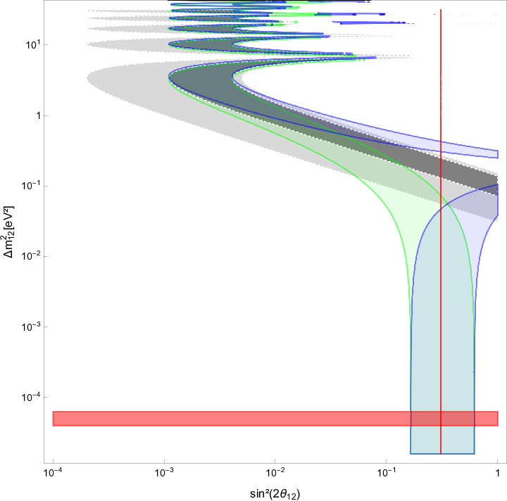
Going further, in fig. (4), we show the allowed region in the parameter space of sin2​(2​θ12)\mbox{sin}^{2}(2\theta_{12}) versus Δ​m122\Delta m_{12}^{2}. Based on an oscillation probability of Pνe→νμ=(2.6±1.5)×10−3P_{\nu_{e}\rightarrow\nu_{\mu}}=(2.6\pm 1.5)\times 10^{-3} from the LSND experiment [2], and using E=60−200​MeVE=60-200\,\mbox{MeV} and x=L≈30​m=2.4×10⁷​eV−1x=L\approx 30\,\mbox{m}=2.4\times 10^{7}\,\mbox{eV}^{-1}, we plot the range of sin2⁡(2​θ12)\sin^{2}(2\theta_{12}) and Δ​m122\Delta m_{12}^{2} values compatible with this result (gray and light gray regions in fig. (4), for 68 %\% C.L. and 95 %\% C.L., respectively). Based on the phenomenological bounds from [17], we consider (Δ​g1​R)12/g≈± 10−10​eV(\Delta g_{1R})_{12}/g\approx\pm\,10^{-10}\,\mbox{eV}, and plotting their contribution in the probability one can see in the figure (4) where the green and blue regions are in contact with long base line (LBL) accelerators results (interception of the red regions), in contrast to the symmetric case (gray regions). It happens due to the smallness of the argument Δ​m1224​π​E\frac{\Delta m_{12}^{2}}{4\pi E}, since that Δ​m1224​π​E≈10−12​eV\frac{\Delta m_{12}^{2}}{4\pi E}\approx 10^{-12}\mbox{eV}. Thereby, the contribution of the mass splitting and DLSB parameter is small and obeys the hierarchy condition π​32​g​(Δ​g1​R)12>Δ​m1224​π​E\frac{\pi\,\sqrt{3}}{2g}\,(\Delta g_{1R})_{12}>\frac{\Delta m_{12}^{2}}{4\pi E}, such way the oscillation length in the eq. (81) can be rewritten as 1ℓ≈3​π2​g​(Δ​g1​R)12\frac{1}{\ell}\approx\frac{\sqrt{3}\pi}{2g}\,\,\left(\Delta g_{1R}\right)_{12}. Finally, one can note that L/ℓ<1L/\ell<1, and due to this property, one can approximate the oscillation probability as:

Pνe→νμS​C​R≈3​π48​sin2⁡(2​θ12)​[L​(Δ​g1​R)12g]2,P^{SCR}_{\nu_{e}\rightarrow\nu_{\mu}}\approx\frac{3\pi^{4}}{8}\sin^{2}(2\theta_{12})\left[\,L\,\frac{(\Delta g_{1R})_{12}}{g}\,\right]^{2}\;, (83)

and using the PDG best fit for sin2​(2​θ12)≈0.31\mbox{sin}^{2}(2\theta_{12})\approx 0.31 and L≈30​mL\approx 30\,\mbox{m}, one finds:

Pνe→νμS​C​R≈6.5×10¹⁵​[(Δ​g1​R)12g]2=(2.6± 1.5)×10−3.P^{SCR}_{\nu_{e}\rightarrow\nu_{\mu}}\approx 6.5\times 10^{15}\,\Bigg[\,\frac{(\Delta g_{1R})_{12}}{g}\,\Bigg]^{2}\!\!=(2.6\,\pm\,1.5)\times 10^{-3}\;. (84)

Therefore, one can infer that |(Δ​g1​R)12g|= 8×10⁻¹⁹\Big|\frac{(\Delta g_{1R})_{12}}{g}\Big|=\,8\times 10^{-19} GeV with 68%\% C.L., the same order of magnitude of the bounds from the tandem model [18], and consistent with our initial assumptions.
Refer to caption
Figure 4: The parameter space of sin2​(2​θ12)\mbox{sin}^{2}(2\theta_{12}) versus Δ​m122\Delta m_{12}^{2} for the eletron-neutrino oscillation. The gray region shows the region with 68%68\% confidence level and the light gray shows the region for the 95%95\% confidence level, according to the LSND experiment. The green and blue regions shows the allowed region for (Δ​g1​R)12/g=10−9​eV(\Delta g_{1R})_{12}/g=10^{-9}\,\mbox{eV} and (Δ​g1​R)12/g=−10−9​eV(\Delta g_{1R})_{12}/g=-10^{-9}\,\mbox{eV} based on the LSND result (68%68\% c.l.). The red region indicates the region with 68%68\% confidence level from the Super-Kamiokande experiment [35].

VI Conclusions

A model with two massive Majorana fermions coupled through self-quartic interactions themselves was proposed in this paper. After a type-II seesaw mechanism, one of the Majorana fermions acquires a light mass (m1)(m_{1}), the other one gains a heavy mass (m2)(m_{2}), and we obtain an effective model with quartic self-interaction fermion theory of axial currents in the physical basis. The model allows the introduction of two auxiliary gauge fields in which the effective potential has a minimum at two vacuum expected values (VEVs) that are constant 44-vectors. These VEVs scales break dynamically the Lorentz symmetry of the model, and as consequence, the dispersion relations of the Majorana fermions are modified.

We calculate the correspondent frequencies solutions for the light and heavy Majorana fermions in the scenarios of time-like and space-like 44-vectors. Posteriorly, we analyze the fluctuations of the auxiliary gauge fields around the VEV scales to calculate the effective action expanded up to second order. Therefore, the radiative corrections yield kinetic terms and mixed mass terms for the gauge fields. The mass matrix is so diagonalized, where the physical eigenstates have one mass of MZ1​R≈6​m1M_{Z_{1R}}\approx\sqrt{6}\,m_{1} for the light gauge field (Z1​R)(Z_{1R}), and a mass of MZ2​R≈6​m2M_{Z_{2R}}\approx\sqrt{6}\,m_{2} for the heavy gauge field (Z2​R)(Z_{2R}). Since we just consider one DLSB parameter, the radiative corrections also generate the Chern-Symons term associated with the heavy gauge field. Using the field equations, we obtain the dispersion relations and the frequency solutions for the gauge fields on a diagonal basis.

To end, we investigate the DLSB in the neutrino’s oscillation. The dispersion relation obtained previously for the light Majorana fermions is used to calculate the transition probability νe→νμ\nu_{e}\rightarrow\nu_{\mu} and the length oscillation. It is well-known that the neutrino oscillation in the electron-muon sector measured by Super-Kamiokande experiment [4] differs from the LSND [2, 3] and the MiniBooNe experiments [9], as can be seen in fig. (1), where one plots the parameter space of sin2​(2​θ12)\mbox{sin}^{2}(2\theta_{12}) versus Δ​m122\Delta m_{12}^{2}. The allowed region for the LSND and the Super-Kamiokande experiments can be seen as the red and gray regions of (1), respectively. The blue and green regions represents the allowed phase space with the contribution of the DLSB parameter with approximate value of (Δ​g1​R)12g≈± 6×10⁻¹⁹\frac{(\Delta g_{1R})_{12}}{g}\approx\pm\,6\times 10^{-19} GeV on the DLSB parameter.

As can be seen in fig. (1), if we admit the light and heavy sector interacts through the axial channel (G3≠0G_{3}\neq 0) only one of the sectors violates dynamically the Lorentz symmetry, and the VEVs scales are given by

a2=3​π2​G2G1​G2−G32andb2=0,\displaystyle a^{2}=\frac{3\pi^{2}\,G_{2}}{G_{1}G_{2}-G_{3}^{2}}\hskip 14.22636pt\mbox{and}\hskip 14.22636ptb^{2}=0\;, (85)

or

a2=0andb2=3​π2​G1G1​G2−G32,\displaystyle a^{2}=0\hskip 14.22636pt\mbox{and}\hskip 14.22636ptb^{2}=\frac{3\pi^{2}\,G_{1}}{G_{1}G_{2}-G_{3}^{2}}\;, (86)

where aμa^{\mu} and bμb^{\mu} couple with the light and heavy sectors, respectively. Thereby, there is a possibility in the phase diagram for the DSLB occurs in the heavy sector maintaining the standard model of the symmetric sector under Lorentz symmetry. One also has that for G3=0G_{3}=0, i.e., in the decoupled scenario, both the VEVs scales can be non-null simultaneously.

If one assumes G3=0G_{3}=0, i.e., the light neutrino sector decouples from the heavy sector, one can estimate the Lorentz violation parameter in the axial neutrino self-interaction. The authors choose this framework since the heavy sector up to date was not detected, which indicates that, if it exists, the heavy sector interacts weakly with the SM particles, particularly with neutrinos. Using the SME limits from ae0=|(aL)e​eT|<2×10⁻²⁷​GeVa^{0}_{e}=|(a_{L})^{T}_{ee}|<2\times 10^{-27}\,\mbox{GeV} (from table D29 of ref. [38]), we obtain the upper bound :

|(aL)μ​μT|≲3×10⁻¹⁸​GeV,|(a_{L})_{\mu\mu}^{T}|\lesssim 3\times 10^{-18}\,\mbox{GeV}\;, (87)

which means the muonic neutrino sector would be the relevant sector in the axial quartic interactions. Based on the experimental results from oscillations of muonic neutrinos [39, 40], which reveals no discrepancies with the standard neutrino oscillation models, one can roughly assume the following hierarchy:

|(aL)e​eT|≪|(aL)μ​μT|≈|(aL)τ​τT|.|(a_{L})_{ee}^{T}|\ll|(a_{L})_{\mu\mu}^{T}|\approx|(a_{L})_{\tau\tau}^{T}|\;. (88)

Is important to comment on the case G3≠0G_{3}\neq 0: If one assumes a more general statement that the light and heavy sectors interact through G3G_{3}, the analysis become much more complex. In fact, any attempt to find any bound assuming G3≠0G_{3}\neq 0 becomes unfeasible with the actual experimental data. In addition to the fact that G2G_{2} and G3G_{3} are constants related to the heavy sector (which one has no information about) more general assumptions should be made, i.e., the full flavor structure of the quartic interactions. These features will be studied in other opportunities.

From the phenomenological point of view, in the high energy limit, the quantity Δ​m2/E\Delta m^{2}/E vanishes and implies that neutrinos at high energy do not oscillate. In the case of DLSB, the oscillation remains even in the high energy limit and can be a motivation to search for oscillation patterns in events from natural astrophysical phenomena which produce particles with energy beyond the PeV scale [41, 42].

Going further, since |a0|∝G1−1/2|a^{0}|\propto G_{1}^{-1/2}, one can roughly estimate the coupling constant for the muon and tau neutrinos : G1(μ)≈G1(τ)≈1034​GeV−2G_{1}^{\,\,(\mu)}\approx G_{1}^{\,\,(\tau)}\approx 10^{34}\,\mbox{GeV}^{-2}. In such a strong coupling environment non-perturbative phenomena may take place and non-linear aspects could drive the system [30]. The effects of this kind of interaction also could be tested in the context of supernova processes and could also generate cosmological implications. These new features will be research subjects in forthcoming papers.

Acknowledgments

Y.M.P.G. is supported by a postdoctoral grant from Fundação Carlos Chagas Filho de Amparo à Pesquisa do Estado do Rio de Janeiro (FAPERJ). M. J. Neves thanks CNPq (Conselho Nacional de Desenvolvimento Científico e Tecnológico), Brazilian scientific support federal agency, for partial financial support, Grant number 313467/2018-8.

References

  • [1] T. Araki et al. (KamLAND Collaboration), Measurement of Neutrino Oscillation with KamLAND: Evidence of Spectral Distortion, Phys. Rev. Lett. 94, 081801 (2005).
  • [2] C. Athanassopoulos et al, Phys. Rev. Lett. 77, 3082 (1996).
  • [3] C. Athanassopoulos et al, Phys. Rev. Lett. 81, 1774 (1998).
  • [4] Y. Fukuda et al. (Super-Kamiokande Collaboration), Evidence for Oscillation of Atmospheric Neutrinos, Phys. Rev. Lett. 81, 1562 (1998).
  • [5] G. Mention, M. Fechner, Th. Lasserre, Th. A. Mueller, D. Lhuillier, M. Cribier and A. Letourneau, The Reactor Antineutrino Anomaly, Phys. Rev. D 83, 073006 (2011).
  • [6] A. Aguilar et al, Evidence for Neutrino Oscillations from the Observation of Electron Anti-neutrinos in a Muon Anti-Neutrino Beam, Phys. Rev. D 64, 112007 (2001).
  • [7] M.V. Smirnov, Zh.J. Hu, J.J. Ling, Yu.N. Novikov, Z. Wang and G. Yang, Sterile neutrino oscillometry with Jinping, The European Physical Journal C 80, 609 (2020).
  • [8] A. A. Aguilar-Arevalo et al (The MiniBooNE Collaboration), A Combined νμ→νe\nu_{\mu}\rightarrow\nu_{e} & ν¯μ→ν¯e\bar{\nu}_{\mu}\rightarrow\bar{\nu}_{e} Oscillation Analysis of the MiniBooNE Excesses, arXiv:hep-exp/1207.4809v2.
  • [9] A. A. Aguilar-Arevalo et al (The MiniBooNE Collaboration), Significant Excess of Electronlike Events in the MiniBooNE Short-Baseline Neutrino Experiment, Phys. Rev. Lett. 121, 221801 (2018).
  • [10] P. Minkowski, μ→e​γ\mu\rightarrow e\,\gamma at a rate of one out of 10910^{9} muon decays?, Phys. Lett. B 67, 421 (1977).
  • [11] R. N. Mohapatra and G. Senjanović, Neutrino Mass and Spontaneous Parity Nonconservation, Phys. Rev. Lett. 44, 912 (1980).
  • [12] R. N. Mohapatra and G. Senjanovic, Neutrino Masses and Mixings in Gauge Models with Spontaneous Parity Violation, Phys. Rev. D 23, 165 (1981).
  • [13] T. Yanagida, Horizontal gauge symmetry and masses of neutrinos, Conf. Proc. C 7902131, 95 (1979).
  • [14] M. Gell-Mann, P. Ramond and R. Slansky, Complex Spinors and Unified Theories, Conf. Proc. C 790927, 315 (1979) [arXiv/hep-th:1306.4669].
  • [15] S. L. Glashow, The Future of Elementary Particle Physics, NATO Sci. Ser. B 61, 687 (1980).
  • [16] T. P. Cheng and L. F. Li, Gauge theory of elementary particle physics, Oxford university press (1994).
  • [17] Kostelecký, V. Alan, and Matthew Mewes. ”Lorentz and CPT violation in neutrinos.” Physical Review D 69.1 (2004): 016005.
  • [18] Teppei Katori, Alan Kostelecky and Rex Tayloe, Global three-parameter model for neutrino oscillations using Lorentz violation, Phys. Rev. D 74, 105009 (2006).
  • [19] Diaz, Jorge S., and V. Alan Kostelecký. ”Lorentz-and C P T-violating models for neutrino oscillations.” Physical Review D 85.1 (2012): 016013.
  • [20] Baruch Rosenstein, Brian J. Warr and Seon H. Park, Dynamical symmetry breaking in four-fermion interaction models, Physics Reports (Review Section of Physics Letters) 205, No. 2 (1991) 59 — 108.
  • [21] Kiyoshi Higashijima, Theory of Dynamical Symmetry Breaking, Progress of Theoretical Physics Supplement No. 104, 1991.
  • [22] M. Pérez-Victoria, Exact Calculation of the Radiatively Induced Lorentz and CPT Violation in QED, Phys. Rev. Lett. 83, 13 (1999).
  • [23] V.A. Miransky, Dynamical symmetry breaking in quantum field theories (World Scientific), (1994).
  • [24] Y. Nambu and G. Jona-Lasinio, Dynamical Model of Elementary Particles Based on an Analogy with Superconductivity, Phys. Rev. 122, 345 (1961).
  • [25] M. Gomes, T. Mariz, J. R. Nascimento, A. J. da Silva, Dynamical Lorentz and CPT symmetry breaking in a 4D four-fermion model. , Phys. Rev. D, 77(10), p. 105002, (2008).
  • [26] J. F. Assunção, T. Mariz, J. R. Nascimento, A. Y. Petrov, Dynamical Lorentz symmetry breaking in a 4D massless four-fermion model. Phys. Rev. D, 96(6), p. 065021, (2017).
  • [27] J. F. Assunção, T. Mariz, J. R. Nascimento, A. Y. Petrov, Dynamical Lorentz symmetry breaking in a tensor bumblebee model., Phys. Rev. D, 100(8), p. 085009, (2019).
  • [28] J. F. Assunção, T. Mariz, J. R. Nascimento, A. Y. Petrov, Induced Chern-Simons modified gravity at finite temperature, J. High Energy Phys., 072 (8), p. 1-13, (2018).
  • [29] B. Charneski, M. Gomes, T. Mariz, J. R. Nascimento, A. J. da Silva, Dynamical Lorentz symmetry breaking in 3D and charge fractionalization, Phys. Rev. D, 79(6), p. 065007, (2009).
  • [30] Y. M. P. Gomes, Dyson-Schwinger equation approach to Lorentz symmetry breaking with finite temperature and chemical potential, Phys. Rev. D 104, 015022 (2021).
  • [31] Sean M. Carroll, George B. Field and Roman Jackiw, Limits on a Lorentz- and parity-violating modification of electrodynamics, Phys. Rev. D 41, 4 (1990).
  • [32] Shinya Kanemura, Toshinori Matsui and Hiroaki Sugiyama, Neutrino mass and dark matter from gauged U​(1)B−LU(1)_{B-L} breaking, Phys. Rev. D 90, 013001 (2014).
  • [33] Pilar Coloma, M. C. Gonzalez-Garciab and Michele Maltoni, Neutrino oscillation constraints on U​(1)′U(1)^{\prime} models: from non-standard interactions to long-range forces, JHEP 01 (2021) 114.
  • [34] Cesar Bonilla, Leon M. G. de la Vega, R. Ferro-Hernandez, Newton Nath and Eduardo Peinado, Neutrino phenomenology in a left-right D​4D4 symmetric model, Phys. Rev. D 102, 036006 (2020).
  • [35] P. A. Zyla et al (Particle Data Group), Prog. Theor. Exp. Phys. 2020, 083C01 (2020).
  • [36] Geoffrey B. Mills et al., Neutrino oscillation results from LSND, Nuclear Physics B - Proceedings Supplements, v. 91, n. 1-3, p. 198-202 (2001).
  • [37] K. ABE et al., Solar neutrino measurements in Super-Kamiokande-IV, Phys. Rev. D 94, 052010 (2016).
  • [38] V. Kostelecký and N. Russell, Data tables for Lorentz and CPT violation, Rev. Mod. Phys. 83 (2011) 11 [0801.0287v13 (2021 edition)].
  • [39] P. Adamson et al. (MINOS+ Collaboration) Precision constraints for three-flavor neutrino oscillations from the full MINOS+ and MINOS dataset, Phys. Rev. Lett. 125, 131802 (2020).
  • [40] M. G. Aartsen et al. (IceCube Collaboration), Determining neutrino oscillation parameters from atmospheric muon neutrino disappearance with three years of IceCube DeepCore data. Phys. Rev. D 91, 072004 (2015).
  • [41] M. G. Aartsen et al. (IceCube Collaboration), First Observation of PeV-Energy Neutrinos with IceCube, Phys. Rev. Lett. 111, 021103 (2013).
  • [42] The IceCube Collaboration, Detection of a particle shower at the Glashow resonance with IceCube, Nature 591, 220-224 (2021).