OrchestRAN: Network Automation through Orchestrated Intelligence in the Open RANEmail: {s.doro, l.bonati, m.polese, melodia}@northeastern.eduThis work was partially supported by the U.S. National Science Foundation under Grants CNS-1923789 and NSF CNS-1925601, and the U.S. Office of Naval Research under Grant N00014-20-1-2132.
Abstract
The next generation of cellular networks will be characterized by softwarized, open, and disaggregated architectures exposing analytics and control knobs to enable network intelligence via innovative data-driven algorithms. How to practically realize this vision, however, is largely an open problem. For a given network optimization/automation objective, it is currently unknown how to select which data-driven models should be deployed and where, which parameters to control, and how to feed them appropriate inputs. In this paper, we take a decisive step forward by presenting and prototyping OrchestRAN, a novel orchestration framework for next generation systems that embraces and builds upon the Open RAN paradigm to provide a practical solution to these challenges. OrchestRAN has been designed to execute in the non-Real-time (RT) RAN Intelligent Controller (RAN) and allows Network Operators (NOs) to specify high-level control/inference objectives (i.e., adapt scheduling, and forecast capacity in near-RT, e.g., for a set of base stations in Downtown New York). OrchestRAN automatically computes the optimal set of data-driven algorithms and their execution location (e.g., in the cloud, or at the edge) to achieve intents specified by the NOs while meeting the desired timing requirements and avoiding conflicts between different data-driven algorithms controlling the same parameters set. We show that the intelligence orchestration problem in Open RAN is NP-hard, and design low-complexity solutions to support real-world applications. We prototype OrchestRAN and test it at scale on Colosseum, the world’s largest wireless network emulator with hardware in the loop. Our experimental results on a network with 7 base stations and 42 users demonstrate that OrchestRAN is able to instantiate data-driven services on demand with minimal control overhead and latency.
Index Terms:
O-RAN, Open RAN, Artificial Intelligence, Orchestration, 5G, 6G.I Introduction
The fifth-generation (5G) of cellular networks and its evolution (NextG), will mark the end of the era of inflexible hardware-based Radio Access Network (RAN) architectures in favor of innovative and agile solutions built upon softwarization, openness and disaggregation principles. This paradigm shift—often referred to as Open RAN—comes with unprecedented flexibility. It makes it possible to split network functionalities—traditionally embedded and executed in monolithic base stations—and instantiate and control them across multiple nodes of the network [1].
In this context, the O-RAN Alliance [2], a consortium led by Network Operators (NOs), vendors and academic partners, is developing a standardized architecture for Open RAN that promotes horizontal disaggregation and standardization of RAN interfaces, thus enabling multivendor equipment interoperability and algorithmic network control and analytics. As shown in Fig. 1, O-RAN embraces the 3rd Generation Partnership Project (3GPP) functional split with Central Units (CUs), Distributed Units (DUs) and Radio Units (RUs) implementing different functions of the protocol stack. O-RAN also introduces (i) a set of open standardized interfaces to interact, control and collect data from every node of the network; as well as (ii) RAN Intelligent Controllers (RANs) that execute third-party applications over an abstract overlay to control RAN functionalities, i.e., xApps in the near-Real-time (RT) and rApps in the non-RT RIC. The O-RAN architecture makes it possible to bring automation and intelligence to the network through Machine Learning (ML) and Artificial Intelligence (AI), which will leverage the enormous amount of data generated by the RAN—and exposed through the O-RAN interfaces—to analyze the current network conditions, forecast future traffic profiles and demand, and implement closed-loop network control strategies to optimize the RAN performance.
For this reason, how to design, train and deploy reliable and effective data-driven solutions has recently received increasing interest from academia and industry alike, with applications ranging from controlling RAN resource and transmission policies [3, 4, 5, 6, 7, 8, 9, 10, 11, 12, 13], to forecasting and classifying traffic and Key Performance Indicators (KPIs) [14, 15, 16, 17, 18], thus highlighting how these approaches will be foundational to the Open RAN paradigm. However, how to deploy and manage, i.e., orchestrate, intelligence into softwarized cellular networks is by no means a solved problem for the following reasons:
Complying with time scales and making input available: Adapting RAN parameters and functionalities requires control loops operating over time scales ranging from a few milliseconds (i.e., real-time) to a few hundreds of milliseconds (i.e., near-RT) to several seconds (i.e., non-RT) [19, 7]. As a consequence, the models and the location where they are executed need to be selected to be able to retrieve the necessary inputs and compute the output within the appropriate time constraints [7, 20]. For instance, while IQ samples are easily available in real time at the RAN, it is extremely hard to make them available at the near-RT and non-RT RICs within the same temporal window, making the execution of models that require IQ samples as input on the RICs ineffective.
Choosing the right model: Each ML/AI model is designed to accomplish specific inference and/or control tasks and requires well-defined inputs in terms of data type and size. One must make sure that the most suitable model is selected for a specific NO request, and that it meets the required performance metrics (e.g., minimum accuracy), delivers the desired inference/control functionalities, and is instantiated on nodes with enough resources to execute it.
Conflict mitigation: One must also ensure that selected ML/AI models do not conflict with each other, and that the same parameter (or functionality) is controlled by only a single model at any given time.
For these reasons, orchestrating network intelligence in the Open RAN presents unprecedented and unique challenges that call for innovative, automated and scalable solutions. In this paper, we address these challenges by presenting OrchestRAN, an automated intelligence orchestration framework for the Open RAN. OrchestRAN follows the O-RAN specifications and operates as an rApp executed in the non-RT RIC (Fig. 1) providing automated routines to: (i) Collect control requests from NOs; (ii) select the optimal ML/AI models to achieve NOs’ goals and avoid conflicts; (iii) determine the optimal execution location for each model complying with timescale requirements, resource and data availability, and (iv) automatically embed models into O-RAN applications that are dispatched to selected nodes, where they are executed and fed the required inputs.
To achieve this goal, we have designed and prototyped novel algorithms embedding pre-processing variable reduction and branching techniques that allow OrchestRAN to compute orchestration solutions with different complexity and optimality trade-offs, while ensuring that the NOs intents are satisfied. We evaluate the performance of OrchestRAN in orchestrating intelligence in the RAN through numerical simulations, and by prototyping OrchestRAN on ColO-RAN [21], an O-RAN-compliant large-scale experimental platform developed on top of Colosseum, the world’s largest wireless network emulator with hardware in-the-loop [22]. Experimental results on an O-RAN-compliant softwarized network with 7 cellular base stations and 42 users demonstrate that OrchestRAN enables seamless instantiation of O-RAN applications with diverse timescale requirements at different O-RAN components. OrchestRAN automatically selects the optimal execution locations for each O-RAN application, thus moving network intelligence to the edge with up to 2.6 reduction of control overhead over the O-RAN E2 interface. To the best of our knowledge, this is the first large-scale demonstration of an O-RAN-compliant network intelligence orchestration system.
II Related Work
The application of ML/AI algorithms to cellular networks is gaining momentum as a promising and effective way to design and deploy solutions capable of predicting, controlling, and automating the network behavior under dynamic conditions. Relevant examples include the application of Deep Learning and Deep Reinforcement Learning (DRL) to predict the network load [23, 14, 9], classify traffic [24, 15, 25], perform beam alignment [16, 17], allocate radio resources [3, 26, 4], and deploy service-tailored network slices [5, 7, 6, 8, 9, 10, 27]. It is clear that ML/AI techniques will play a key role in the transition to intelligent networks, especially in the O-RAN ecosystem [28]. However, a relevant challenge that still remains unsolved is how to bring such intelligence to the network in an efficient, reliable and automated way, which is ultimately the goal of this paper.
In [29], Ayala-Romero et al. present an online Bayesian learning orchestration framework for intelligent virtualized RANs where resource allocation follow channel conditions and network load. The same authors present a similar framework in [11], where networking and computational resources are orchestrated via DRL to comply with service level agreements (SLAs) while accounting for the limited amount of resources. Singh et al. present GreenRAN, an energy-efficient orchestration framework for NextG that splits and allocates RAN components according to the current resource availability [30]. In [31], Chatterjee et al. present a radio resource orchestration framework for 5G applications where network slices are dynamically re-assigned to avoid inefficiencies and SLA violations. Relevant to our work are the works of Morais et al. [32] and Matoussi et al. [33], which present frameworks to optimally disaggregate, place and orchestrate RAN components in the network to minimize computation and energy consumption while accounting for diverse latency and performance requirements. Although the above works all present orchestration frameworks for NextG systems, they are focused on orchestrating RAN resources and functionalities, rather than network intelligence, which represents a substantially different problem.
In the context of orchestrating ML/AI models in NextG systems, Baranda et al. [34, 35] present an architecture for the automated deployment of models in the 5Growth management and orchestration (MANO) platform [36], and demonstrate automated instantiation of models on demand. The closest to our work is the work of Salem et al. [20], which proposes an orchestrator to select and instantiate inference models at different locations of the network to obtain a desirable balance between accuracy and latency. However, [20] is not concerned with O-RAN systems, but focuses on data-driven solutions for inference in cloud-based applications.
Besides the differences highlighted in the previous discussion, OrchestRAN differs from the above works in that it focuses on the Open RAN architecture and is designed to instantiate both inference and control solutions complying with O-RAN specifications. Moreover, OrchestRAN allows model sharing across multiple requests to efficiently reuse available network resources. We prototyped and benchmarked OrchestRAN on Colosseum. To the best of our knowledge, this is the first large-scale demonstration of a network intelligence orchestration system tailored to O-RAN architecture and networks.
III O-RAN: A Primer
O-RAN embraces the 7-2x functional split (an extension of the 3GPP 7-2 split), where network functionalities are divided across multiple nodes, namely, CUs, DUs and RUs (Fig. 1, left). The RUs implement lower physical layer functionalities. The DUs interact with the RUs via the Open Fronthaul interface and implement functionalities pertaining to both the higher physical layer and the MAC layer. Finally, the remaining functionalities of the protocol stack are implemented and executed in the CU. The latter is connected to the DUs through the F1 interface and is further split in two entities—handling control and user planes—connected via the E1 interface. These network elements run on “white-box” hardware components connected through O-RAN open interfaces, thus enabling multivendor interoperability and overcoming the vendor lock-in [1].
Beyond disaggregation, the main innovation introduced by O-RAN lies in the non-RT and near-RT RICs. These components enable dynamic and softwarized control of the RAN, as well as the collection of statistics via a publish-subscribe model [37] through open and standardized interfaces, e.g., the O1 and E2 interfaces (Fig. 1, left). Specifically, the near-RT RIC hosts applications (xApps) that implement time-sensitive—i.e., between 10 ms and 1 s—operations to perform closed-loop control over the RAN elements. Practical examples include control of load balancing, handover procedures, scheduling and RAN slicing policies [7, 38, 39, 40]. The non-RT RIC, instead, is designed to execute within a service management and orchestration (SMO) framework, e.g., Open Network Automation Platform (ONAP), and acts at time scales above 1 s. It takes care of training ML/AI models, as well as deploying models and network control policies on the near-RT RIC through the A1 interface. Similar to its near-RT counterpart, the non-RT RIC supports the execution of third-party applications, called rApps. These components act in concert to gather data and performance metrics from the RAN, and to optimize and reprogram its behavior in real time through software algorithms to reach NO’s goals. O-RAN specifications also envision ML/AI models instantiated directly on the CUs and DUs, implementing RT—Transmission Time Interval (TTI) level—control loops that operate on 10 ms time-scales [41]. Although these are left for future O-RAN extensions, OrchestRAN has been natively designed to support such control loops, implementing RT applications, which we will refer to as dApps to avoid confusion.
IV OrchestRAN
As illustrated in Fig. 1, OrchestRAN is designed to be executed as an rApp at the non-RT RIC. Its architecture is illustrated in Fig. 2. At a high-level, first NOs specify their intent by submitting a control request to OrchestRAN (step I). This includes the set of functionalities they want to deploy (e.g., network slicing, beamforming, scheduling control, etc.), the location where functionalities are to be executed (e.g., RIC, CU, DU) and the desired time constraint (e.g., delay-tolerant, low-latency). Then, requests are gathered by the Request Collector (step II, Section IV-C) and fed to the Orchestration Engine (step III, Section IV-D) which: (i) Accesses the ML/AI Catalog (Section IV-B) and the Infrastructure Abstraction module (Section IV-A) to determine the optimal orchestration policy and models to be instantiated; (ii) automatically creates containers with the embedded ML/AI models in the form of O-RAN applications, and (iii) dispatches such applications at the locations determined by the Orchestration Engine.

IV-A The Infrastructure Abstraction Module
This module provides a high-level representation of the physical RAN architecture, which is divided into five separate logical groups: non-RT RICs, near-RT RICs, CUs, DUs and RUs. Each group contains a different number of nodes deployed at different locations of the network. Let be the set of such nodes, and be their number.
The hierarchical relationships between nodes can be represented via an undirected graph with a tree structure such as the one in Fig. 1 (right). Specifically, leaves represent nodes at the edge (e.g., RUs/DUs/CUs), while the non-RT RIC is the root of the tree.11 1 Coexisting CUs/DUs/RUs are modeled as a single logical node with a hierarchy level equal to that of the hierarchically highest node in the group. For any two nodes , we define variable such that if node is reachable from node (e.g., there exist a communication link such that node can forward data to node ), otherwise. In practical deployments, it is reasonable to assume that nodes on different branches of the tree are unreachable. Moreover, for each node , let be the total amount of resources of type dedicated to hosting and executing ML/AI models and their functionalities, where represents the set of all resource types. Although we do not make any assumptions on the specific types of resources, practical examples may include the number of CPUs, GPUs, as well as available disk storage and memory. In the following, we assume that each non-RT RIC identifies an independent networking domain and the set of nodes includes near-RT RICs, CUs, DUs and RUs controlled by the corresponding non-RT RIC only.
IV-B The ML/AI Catalog
In OrchestRAN, the available pre-trained data-driven solutions are stored in a ML/AI Catalog consisting of a set of ML/AI models. Let be the set of all possible control and inference functionalities (e.g., scheduling, beamforming, capacity forecasting, handover prediction) offered by such ML/AI models—hereafter referred to simply as “models”.
Let and . For each model , represents the subset of functionalities offered by . Accordingly, we define a binary variable such that if , otherwise. We use to indicate the amount of resources of type required to instantiate and execute model . Let be the set of possible input types. For each model , represents the type of input required by the model (e.g., IQ samples, throughput and buffer size measurements).
Naturally, not all models can be equally executed everywhere. For example, a model performing beam alignment [16], in which received IQ samples are fed to a neural network to determine the beam direction, can only execute on nodes where IQ samples are available. While IQ samples can be accessed in real-time at the RU, they are unlikely to be available at CUs and the RICs without incurring in high overhead and transmission latency. For this reason, we introduce a suitability indicator which specifies how well a model is suited to provide a specific functionality when instantiated on node . Values of closer to 1 mean that the model is well-suited to execute at a specific location, while values closer to 0 indicate that the model performs poorly. We also introduce a performance score measuring the performance of the model with respect to . Typical performance metrics include classification/forecasting accuracy, mean squared error and probability of false alarm. A model can be instantiated on the same node multiple times to serve different NOs or traffic classes. However, due to limited resources, each node supports at most instances of model , where is the floor operator.
IV-C Request Collector
OrchestRAN allows NOs to submit requests specifying which functionalities they require, where they should execute, and the desired performance and timing requirements. Without loss of generality, we assume that each request is feasible. The Request Collector of OrchestRAN is in charge of collecting such requests. A request is defined as a tuple , with each element defined as follows:
Functions and locations. For each request , we define the set of functionalities that must be instantiated on the nodes as , with . Required functionalities and nodes are specified by a binary indicator such that if request requires functionality on node , i.e., , otherwise. We also define as the subset of nodes of the network where functionalities in should be offered;
Performance requirements. For any request , indicates the minimum performance requirements that must be satisfied to accommodate . For example, if is a beam detection functionality, can represent the minimum detection accuracy of the model. We do not make any assumptions on the physical meaning of as it reasonably differs from one functionality to the other.
Timing requirements. Some functionalities might have strict latency requirements that make their execution at nodes far away from the location where the input is generated impractical or inefficient. For this reason, represents the maximum latency request can tolerate in executing on ;
Data source. For each request , the NO also specifies the subset of nodes whose generated (or collected) data must be used to deliver functionality on node . This set is defined as , where . This information is paramount to ensure that each model is fed with the proper data generated by the intended sources only. For any tuple we assume that for all .
In the remaining of this paper, we use to represent the set of outstanding requests with being their number.
IV-D The Orchestration Engine
As depicted in Fig. 3, once requests are submitted to OrchestRAN, the Orchestration Engine selects the most suitable models from the ML/AI Catalog and the location where they should execute (step I). Then, OrchestRAN embeds the models into containers (e.g., Docker containers of dApps, xApps, rApps) (step II) and dispatches them to the selected nodes (step III). Here, they are fed data from the RAN and execute their functionalities (step IV). The selection of the models and of their optimal execution location is performed by solving the orchestration problem discussed in detail in Sections V and VI. This results in an orchestration policy, which is converted into a set of O-RAN applications that are dispatched and executed at the designated network nodes, as discussed next.
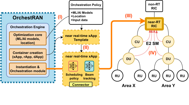
Container creation, dispatchment and instantiation. To embed models in different O-RAN applications, containers integrate two subsystems, which are automatically compiled from descriptive files upon instantiation. The first is the model itself, and the second is an application-specific connector. This is a library that interfaces with the node where the application is running (i.e., with the DU in the case of dApps, near-RT RIC for xApps, and non-RT RIC for rApps), collects data from and sends control commands to nodes in . Once the containers are generated, OrchestRAN dispatches them to the proper endpoints specified in the orchestration policy, where are instantiated and interfaced with the RAN to receive input data. For example, xApps automatically send an E2 subscription request to nodes in , and use custom Service Models (SMs) to interact with them over the E2 interface [37] (see Fig. 3).
V The Orchestration Problem
Before formulating the orchestration problem, we first discuss important properties of Open RAN systems.
Functionality outsourcing. Any functionality that was originally intended to execute at node can be outsourced to any other node as long as . As we will discuss next, the node hosting the outsourced model must have access to the required input data, have enough resources to instantiate and execute the outsourced model, and must satisfy performance and timing requirements of the original request.
Model sharing. The limited amount of resources, especially at DUs and RUs, calls for efficient resource allocation strategies. If multiple requests involve the same functionalities on the same group of nodes, an efficient approach consists in deploying a single model that can be shared across all requests.
For the sake of clarity, in Fig. 4 (left) we show an example where a request can be satisfied by instantiating models and on , and a second one that can be accommodated by instantiating models and on . Fig. 4 (right) shows an alternative solution where (common to both requests) is outsourced to and it is shared between the two requests, with a total of three deployed models, against the four required in Fig. 4 (left). In the next section, we also discuss the case where model sharing or function outsourcing are nonviable.

V-A Formulating the Orchestration Problem
Let be a binary variable such that if functionality demanded by request on node is provided by instance of model instantiated on node . In the following, we refer to the variable as the orchestration policy, where .
Conflict avoidance. For any tuple such that , we assume that OrchestRAN can instantiate at most one model to avoid multiple models controlling the same parameters and/or functionalities. As mentioned earlier, this can be achieved by either instantiating the model at , or by outsourcing it to another node . The above requirement can be formalized as follows:
| (1) |
where indicates whether or not is satisfied. Specifically, (1) ensures that: (i) For any tuple such that , function is provided by one model only, and (ii) (i.e., request is satisfied) if and only if OrchestRAN deploys models providing all functionalities specified in .
Complying with the requirements. An important aspect of the orchestration problem is guaranteeing that the orchestration policy satisfies the minimum performance requirements of each request , and that both data collection and execution procedures do not exceed the maximum latency constraint . These requirements are captured by the following constraints.
V-A1 Quality of models
For each tuple such that , NOs can specify a minimum performance level . This can be enforced via the following constraint
| (2) |
where , and the performance score is defined in Section IV-B. In (2), if the goal is to guarantee a value of higher than a minimum performance level , and if the goal is to keep below a maximum value .
V-A2 Control-loop time-scales
Each model requires a specific type of input and, for each tuple , we must ensure that the time needed to collect such input from nodes in does not exceed . For each orchestration policy , the data collection time can be formalized as follows:
| (3) |
where , is the input size of model measured in bytes, is the data rate of the link between nodes and , and represents the propagation delay between nodes and . Let be the time to execute model on node . For any tuple , the execution time under orchestration policy is
| (4) |
By combining (3) and (4), any orchestration policy must satisfy the following constraint for all tuples:
| (5) |
Avoiding resource over-provisioning. We must guarantee that the resources consumed by the O-RAN applications do not exceed the resources of type available at each node (i.e., ). For each and , we have
| (6) |
where indicates whether instance of model is associated to at least one model on node . Specifically, let
| (7) |
be the number of tuples assigned to instance of model on node ( implies that is shared). Notice that (6) and (7) are coupled one to another as if and only if . This conditional relationship can be formulated by using the following big-M formulation [42]
| (8) | ||||
| (9) |
where is a real-valued number whose value is larger than the maximum value of , i.e., [42].
Problem formulation. For any request , let represent its value. The goal of OrchestRAN is to compute an orchestration policy maximizing the total value of requests being accommodated by selecting (i) which requests can be accommodated; (ii) which models should be instantiated; and (iii) where they should be executed to satisfy request performance and timescale requirements. This can be formulated as
| (10) | ||||
| (11) | ||||
| (12) | ||||
| (13) |
where is the orchestration policy, and . A particularly relevant case is that where for all , i.e., the goal of OrchestRAN is to maximize the number of satisfied requests.
Disabling model sharing. Indeed, model sharing allows a more efficient use of the available resources. However, out of privacy and business concerns, NOs might not be willing to share O-RAN applications. In this case, model sharing can be disabled in OrchestRAN by guaranteeing that a model is assigned to one request only. This is achieved by adding the following constraint for any , and
| (14) |
V-B NP-hardness of the Orchestration Problem
VI Solving the Orchestration Problem
BILP problems such as Problem (10) can be optimally solved via Branch-and-Bound (B&B) techniques [44], readily available within well-established numerical solvers, e.g., CPLEX, MATLAB, Gurobi. However, due to the extremely large number of optimization variables, these solvers might still fail to compute an optimal solution in a reasonable amount of time, especially in large-scale deployments. Indeed, , where , , , and . For example, a deployment with , , , and involves 106 optimization variables.
VI-A Combating Dimensionality via Variable Reduction
To mitigate the “curse of dimensionality” of the orchestration problem, we have developed two pre-processing algorithms to reduce the complexity of Problem (10) while guaranteeing the optimality of the computed solutions. We leverage a technique called variable reduction [45]. This exploits the fact that, due to constraints and structural properties of the problem, there might exist a subset of inactive variables whose value is always zero. These variables do not participate in the optimization process, yet they increase its complexity. To identify those variables, we have designed the following two techniques.
Function-aware Pruning (FP). It identifies the set of inactive variables , which contains all the variables such that either (i) , i.e., request does not require function at node , or (ii) , i.e., model does not offer function ;
Architecture-aware Pruning (AP). This procedure identities those variables whose activation results in instantiating a model on a node that cannot receive input data from nodes in . Indeed, for a given tuple such that , we cannot instantiate any model on a node such that , i.e., the two nodes are not connected. The set of these inactive variables is defined as .
Once we have identified all inactive variables, Problem (10) is cast into a lower-dimensional space where the new set of optimization variables is equal to , which still guarantees the optimality of the solution [45]. The impact of these procedures on the complexity of the orchestration problem will be investigated in Section VII.
VI-B Graph Tree Branching
Notice that , i.e., the number of variables of the orchestration problem grows quadratically in the number of nodes. Since the majority of nodes of the infrastructure are RUs, DUs and CUs, it is reasonable to conclude that these nodes are the major source of complexity. Moreover, O-RAN systems operate following a cluster-based approach where each near-RT RIC controls a subset of CUs, DUs and RUs of the network only, i.e., a cluster, which have none (or limited) interactions with nodes from other clusters.
These two intuitions are the rationale behind the low-complexity and scalable solution proposed in this section, which consists in splitting the infrastructure tree into smaller subtrees—each operating as an individual cluster—and creating sub-instances of the orchestration problem that only accounts for requests and nodes regarding the considered subtree. The main steps of this algorithm are:
Step I: Let be the number of near-RT RICs in the non-RT RIC domain. For each cluster , the -th subtree is defined such that and , with being the non-RT RIC. A variable is used to determine whether a node belongs to cluster (i.e., ) or not (i.e., ). Since, , we have that for any ;
Step II: For each subtree we identify the subset such that contains all the requests that involve nodes belonging to cluster only;
Step III: We solve Problem (10) via B&B considering only requests in and nodes in . The solution is a tuple specifying which models are instantiated and where (), which requests are satisfied in cluster () and what instances of the models are instantiated on each node of ().
Remark. This branching procedure might compute solutions with partially satisfied requests. These are requests that are accommodated on a subset of clusters only, which violates Constraint 1. However, as we will show in Section VII, this procedure is scalable as each subtree involves a limited number of nodes only, and we can solve each lower-dimensional instance of Problem (10) in parallel and in less than 0.1 s.
VII Numerical Evaluation
| non-RT RIC | near-RT RIC | CU | DU | RU | |
| All nodes (ALL) | ✓ | ✓ | ✓ | ✓ | ✓ |
| Edge and RAN (ER) | ✗ | ✓ | ✓ | ✓ | ✓ |
| RAN only (RO) | ✗ | ✗ | ✓ | ✓ | ✓ |
| TTI-level - 0.01s | Sub-second - 1s | Long - 1s | |
| Delay-Tolerant (DT) | 0.2 | 0.2 | 0.6 |
| Low Latency (LL) | 0.2 | 0.6 | 0.2 |
| Ultra-Low Latency (ULL) | 0.6 | 0.4 | 0 |
To evaluate the performance of OrchestRAN in large-scale scenarios, we have developed a simulation tool in MATLAB that uses CPLEX to execute optimization routines. For each simulation, NOs submit randomly generated requests, each specifying multiple sets of functionalities and nodes, as well as the desired timescale. Unless otherwise stated, we consider a single-domain deployment with 1 non-RT RIC, 4 near-RT RICs, 10 CUs, 30 DUs and 90 RUs. For each simulation, the number of network nodes is fixed, but the tree structure of the infrastructure is randomly generated. We consider the three cases shown in Table II, where we limit the type of nodes that can be included in each request. Similarly, we also consider the three cases in Table II. For each case, we specify the probability that the latency requirement for each tuple is associated to a specific timescale. The combination of these 6 cases covers relevant Open RAN applications.
The ML/AI Catalog consists of models that provide different functionalities. Ten models use metrics from the RAN (e.g., throughput and buffer measurements) as input, while the remaining three models are fed with IQ samples from RUs. The input size is set to 100 and 1000 bytes for the metrics and IQ samples, respectively. For the sake of illustration, we assume that , and for all , , and . The execution time of each model is equal across all models and nodes and set to ms. The available bandwidth is 100 Gbps between non-RT RIC and near-RT RIC, 50 Gbps between near-RT RICs and CUs, 25 Gbps between CUs and DUs, and 20 Gbps between DUs and RUs, while the propagation delay is set to ms, respectively. The resources available at each node are represented by the number of available CPU cores, and we assume that each model requests one core only, i.e., . The number of cores available at non-RT RICs, near-RT RICs, CUs, DUs and RUs are 128, 8, 4, 2, and 1, respectively. Results presented in this section are averaged over 100 independent simulation runs.
Computational complexity. Fig. 5 shows the number of optimization variables and computation time of our algorithms with varying network size. At each simulation run, we consider a single non-RT RIC and a randomly generated tree graph that matches the considered size. As expected, the number of variables and the complexity increase with larger networks. This can be mitigated by using our FP and AP pre-processing algorithms, which reduce the number of optimization variables while ensuring the optimality of the computed solution. Their combination allows computation of optimal solutions in 0.1 s and 2 s for networks with 200 and 500 nodes, respectively. Fig. 5 also shows the benefits of branching the optimization problem into sub-problems of smaller size (Section VI-B).
Although the branching procedure might produce partially satisfied requests, it results in a computation time lower than 0.1 s even for instances with 2000 nodes, providing a fast and scalable solution for large-scale applications.
Acceptance ratio. Fig. 6 (left) shows the acceptance ratio for different cases and algorithms. The number of accepted requests decreases when moving from loose timing requirements (i.e., Delay-tolerant (DT)), to tighter ones (i.e., Low Latency (LL) and Ultra-Low Latency (ULL)). For example, while 95% of requests are satisfied on average for the DT configuration, we observe ULL instances in which only 70% of requests are accepted. Indeed, TTI-level services may only be possible at the DUs/RUs which, however, have limited resources and cannot support the execution of many concurrent O-RAN applications. In Fig. 6 (right), we show the probability that a request is partially accepted when considering the branching algorithm. Specifically, it shows that branching results in 99% of requests being partially satisfied on one subtree or more. This means that in the case where not enough resources are available to accept the entirety of the request, OrchestRAN can satisfy portions of it. Thus, requests that would be otherwise rejected can be at least partially accommodated.
Advantages of model sharing. Fig. 7 shows the resource utilization with and without model sharing (left) and the corresponding resource utilization saving (right). As expected, model sharing always results in lower resource utilization and uses 2 less resources than the case without model sharing. Fig. 9 shows the acceptance ratio when model sharing is disabled, and by comparing it with Fig. 6 (left)—where model sharing is enabled—we notice that model sharing also increases the acceptance ratio. Specifically, model sharing accommodates at least 90% of requests in all cases, while this number drops to 70% when model sharing is disabled.
To better understand how OrchestRAN orchestrates intelligence, Fig. 9 shows the distribution of models across the different network nodes for the ER case (see Table II) with different timing constraints. Requests with loose timing requirements (DT) result in 45% of models being allocated in the RICs. Instead, stringent timing constraints (LL and ULL) result in 70% of models being instantiated at CUs, DUs, and RUs.
VIII Prototype and Experimental Evaluation
To demonstrate the effectiveness of OrchestRAN, we leveraged ColO-RAN [21], an O-RAN-compliant large-scale experimental platform developed on top of the Colosseum wireless network emulator [22]. Colosseum includes 128 computing servers (i.e., Standard Radio Nodes (SRNs)), each controlling a USRP X310 Software-defined Radio (SDR), and a Massive Channel Emulator (MCHEM) emulating wireless channels between the SRNs to reproduce realistic and time-varying wireless characteristics (e.g., path-loss, multi-path) under different deployments (e.g., urban, rural, etc.) [22]. We leverage the publicly available tool SCOPE [26] to instantiate a softwarized cellular network with 7 base stations and 42 User Equipments (UEs) (6 UEs per base station) on the Colosseum city-scale downtown Rome scenario, and to interface the base stations with the O-RAN near-RT RIC through the E2 interface. SCOPE, which is based on srsRAN [46], implements open Application Programming Interfaces (APIs) to reconfigure the base station parameters (e.g., slicing resources, scheduling policies, etc.) from O-RAN applications through closed-control loops, and to automatically generate datasets from RAN statistics (e.g., throughput, buffer size, etc.). Users are deployed randomly and generate traffic belonging to 3 different network slices configured as follows: (i) slice 0 is allocated an Enhanced Mobile Broadband (eMBB) service, in which each UE requests 4 Mbps constant bitrate traffic; (ii) slice 1 a Machine-type Communications (MTC) service, in which each UE requests Poisson-distributed traffic with an average rate of 45 kbps, and (iii) slice 2 to a Ultra Reliable and Low Latency Communication (URLLC) service, in which each UE requests Poisson-distributed traffic with an average rate of 90 kbps. We assume 2 UEs per slice, whose traffic is handled by the base stations, which use a 10 MHz channel bandwidth with 50 Physical Resource Block (PRB).
| Reward | ||||
| Slice 0 | Slice 1 | Slice 2 | Actions | |
| M3 | max(Throughput) | max(TX pkts) | max(PRB ratio) | Scheduling |
| M4 | max(Throughput) | max(TX pkts) | min(Buffer size) | Scheduling, RAN slicing |
The high-level architecture of the OrchestRAN prototype on Colosseum is shown in Fig. 10. OrchestRAN runs in an Linux Container (LXC) embedding the components of Fig 2. For each experiment, we randomly generate a new set of control requests every 4 minutes. The Orchestration Engine computes the optimal orchestration policy and embeds the models within O-RAN applications that are dispatched to the nodes where they are executed. We consider the case where models can run at the near-RT RIC (as xApps) or at the DU (as dApps via SCOPE).

We used SCOPE to generate datasets on Colosseum and train 4 ML models that constitute our ML/AI Catalog. Models and have been trained to forecast throughput and transmission buffer size.22 2 Due to space limitations, and since the goal of this paper is focused on how to orchestrate pre-trained models to accomplish NOs goals, details on the training procedures are omitted. Models and control the parameters of the network to maximize different rewards through Proximal Policy Optimization (PPO)-based DRL agents (see Table III). Specifically, consists of three DRL agents, each making decisions on the scheduling policies of one slice only. The three agents aim at maximizing the throughput of slice 0, the number of transmitted packets of slice 1, and the ratio between the allocated and requested PRBs (i.e., the PRB ratio which takes values in ) of slice 2, respectively. Model , instead, consists of a single DRL agent controlling the scheduling and RAN slicing policies (i.e., how many PRBs are assigned to each slice) to jointly maximize the throughput of slice 0 and the number of transmitted packets of slice 1, and to minimize the buffer size of slice 2. Each model requires one CPU core, and we consider three configurations: (i) “RIC only”, in which models can be executed via xApps at the near-RT RIC only; (ii) “RIC + lightweight DU”, in which DUs have 2 cores each to execute up to two dApps concurrently; and (iii) “RIC + powerful DU”, in which DUs are equipped with 8 cores. In all cases, the near-RT RIC has access to 50 cores. Overall, we ran more than 95 hours of experiments on Colosseum.
Experimental results. Fig. 11 (left) shows the probability that models are executed at the near-RT RIC for different configurations and number of requests. As expected, in the “RIC only” case, all models execute as xApps at the near-RT RIC, while both “RIC + lightweight DU ” and “RIC + powerful DU ” cases result in 25% of models executing at the RIC. The remaining 75% of the models are executed as dApps at the DUs.
Fig. 11 (right) shows the traffic in Mbyte over the E2 interface between the near-RT RIC and the DUs for the different configurations. This includes messages to set up the initial subscription between the near-RT RIC and the DUs, messages to report metrics from the DUs to the RIC (e.g., throughput, buffer size), and control messages from the RIC to the DUs (e.g., to update scheduling and RAN slicing policies). Results clearly show that 40% of the E2 traffic transports payload information (dark bars), while the remaining 60% consists of overhead data. Although the initial subscription messages exchanged between the near-RT RIC and the DUs are sent in all considered cases, running models as dApps at the DUs still results in up to 2.6 less E2 traffic if compared to the “RIC only” case.

Finally, we showcase the impact of the real-time execution of OrchestRAN on the network performance. We focus on DU 7, and in Fig. 12 (top) we show the location and time instant at which OrchestRAN instantiates the four models on the near-RT RIC and on DU 7 for a single experiment. The impact on the network performance of the different orchestration policies is shown in Fig. 12 (center and bottom). Since and perform forecasting tasks only, the figure only reports the evolution of the metrics used to reward the DRL agents and (see Table III) for different slices. We notice that OrchestRAN allows the seamless instantiation of dApps and xApps, controlling the same DU without causing any service interruptions. Moreover, although and share the same reward for slices 0 and 1, can also make decisions on the network slicing policies. Thus, it provides a higher throughput for slice 0 (10% higher than ), and a higher number of transmitted packets for slice 1 (2 higher than ) (Fig. 12 (center)). Similarly, in the case of slice 2, aims at maximizing the PRB ratio, while at minimizing the size of the transmission buffer, which results in and computing different control policies for slice 2. As shown Fig. 12 (bottom), although converges to a stable control policy that results in a PRB ratio 1, its buffer size is higher than that of . Conversely, the buffer size of slice 2 decreases once is instantiated with a decrease in the PRB ratio.
IX Conclusions
In this paper, we presented OrchestRAN, a novel network intelligence orchestration framework for Open RAN systems. OrchestRAN is based upon O-RAN specifications and leverages the RIC xApps and rApps and O-RAN open interfaces to provide NOs with an automated orchestration tool for deploying data-driven inference and control solutions with diverse timing requirements. OrchestRAN has been equipped with orchestration algorithms with different optimality/complexity trade-offs to support non-RT, near-RT and RT applications. We assessed OrchestRAN performance and presented an O-RAN-compliant prototype by instantiating a cellular network with 7 base stations and 42 UEs on the Colosseum network emulator. Our experimental results demonstrate that OrchestRAN achieves seamless instantiation of O-RAN applications at different network nodes and time scales, and reduces the message overhead over the O-RAN E2 interface by up to 2.6 when instantiating intelligence at the edge of the network.
References
- [1] L. Bonati, M. Polese, S. D’Oro, S. Basagni, and T. Melodia, “Open, Programmable, and Virtualized 5G Networks: State-of-the-Art and the Road Ahead,” Computer Networks, vol. 182, pp. 1–28, Dec. 2020.
- [2] O-RAN WG1, “O-RAN Architecture Description - v2.00,” Technical Specification, 2020.
- [3] J. Du, C. Jiang, J. Wang, Y. Ren, and M. Debbah, “Machine Learning for 6G Wireless Networks: Carrying Forward Enhanced Bandwidth, Massive Access, and Ultrareliable/Low-Latency Service,” IEEE Vehicular Technology Magazine, vol. 15, no. 4, pp. 122–134, 2020.
- [4] S. Shen, T. Zhang, S. Mao, and G.-K. Chang, “DRL-Based Channel and Latency Aware Radio Resource Allocation for 5G Service-Oriented RoF-mmWave RAN,” Journal of Lightwave Technology, 2021.
- [5] A. Okic, L. Zanzi, V. Sciancalepore, A. Redondi, and X. Costa-Pérez, “-ROAD: a Learn-as-You-Go Framework for On-Demand Emergency Slices in V2X Scenarios,” in Proc. of IEEE INFOCOM, 2021.
- [6] D. Bega, M. Gramaglia, A. Garcia-Saavedra, M. Fiore, A. Banchs, and X. Costa-Perez, “Network Slicing Meets Artificial Intelligence: An AI-based Framework for Slice Management,” IEEE Communications Magazine, vol. 58, no. 6, pp. 32–38, 2020.
- [7] L. Bonati, S. D’Oro, M. Polese, S. Basagni, and T. Melodia, “Intelligence and Learning in O-RAN for Data-driven NextG Cellular Networks,” IEEE Communications Magazine, vol. 59, no. 10, pp. 21–27, October 2021.
- [8] S. Bakri, P. A. Frangoudis, A. Ksentini, and M. Bouaziz, “Data-Driven RAN Slicing Mechanisms for 5G and Beyond,” IEEE Trans. on Network and Service Management, 2021.
- [9] N. Salhab, R. Langar, R. Rahim, S. Cherrier, and A. Outtagarts, “Autonomous Network Slicing Prototype Using Machine-Learning-Based Forecasting for Radio Resources,” IEEE Communications Magazine, vol. 59, no. 6, pp. 73–79, 2021.
- [10] J. Mei, X. Wang, K. Zheng, G. Boudreau, A. B. Sediq, and H. Abou-zeid, “Intelligent Radio Access Network Slicing for Service Provisioning in 6G: A Hierarchical Deep Reinforcement Learning Approach,” IEEE Trans. on Communications, 2021.
- [11] J. A. Ayala-Romero, A. Garcia-Saavedra, M. Gramaglia, X. Costa-Perez, A. Banchs, and J. J. Alcaraz, “vrAIn: Deep Learning based Orchestration for Computing and Radio Resources in vRANs,” IEEE Trans. on Mobile Computing, 2020.
- [12] L. Bonati, S. D’Oro, L. Bertizzolo, E. Demirors, Z. Guan, S. Basagni, and T. Melodia, “CellOS: Zero-touch Softwarized Open Cellular Networks,” Computer Networks, vol. 180, pp. 1–13, Oct. 2020.
- [13] B. Casasole, L. Bonati, S. D’Oro, S. Basagni, A. Capone, and T. Melodia, “QCell: Self-optimization of Softwarized 5G Networks through Deep Q-learning,” in Proc. of IEEE GLOBECOM, 2021.
- [14] D. Bega, M. Gramaglia, M. Fiore, A. Banchs, and X. Costa-Perez, “DeepCog: Optimizing Resource Provisioning in Network Slicing with AI-based Capacity Forecasting,” IEEE Journal on Selected Areas in Communications, vol. 38, no. 2, pp. 361–376, 2019.
- [15] U. Paul, J. Liu, S. Troia, O. Falowo, and G. Maier, “Traffic-profile and Machine Learning Based Regional Data Center Design and Operation for 5G Network,” Journal of Comm. and Networks, vol. 21, no. 6, 2019.
- [16] M. Polese, F. Restuccia, and T. Melodia, “DeepBeam: Deep Waveform Learning for Coordination-Free Beam Management in mmWave Networks,” Proc. of ACM MobiHoc, 2021.
- [17] A. Klautau, P. Batista, N. González-Prelcic, Y. Wang, and R. W. Heath, “5G MIMO Data for Machine Learning: Application to Beam-selection Using Deep Learning,” in Proc. of ITA Workshop, 2018.
- [18] C. Luo, J. Ji, Q. Wang, X. Chen, and P. Li, “Channel State Information Prediction for 5G Wireless Communications: A Deep Learning Approach,” IEEE Trans. on Network Science and Engineering, vol. 7, no. 1, pp. 227–236, 2018.
- [19] J. M. DeAlmeida, L. DaSilva, C. B. Bonato Both, C. G. Ralha, and M. A. Marotta, “Artificial Intelligence-Driven Fog Radio Access Networks: Integrating Decision Making Considering Different Time Granularities,” IEEE Vehicular Technology Magazine, 2021.
- [20] T. S. Salem, G. Castellano, G. Neglia, F. Pianese, and A. Araldo, “Towards Inference Delivery Networks: Distributing Machine Learning with Optimality Guarantees,” in Proc. of IEEE MedHocNet, 2021.
- [21] M. Polese, L. Bonati, S. D’Oro, S. Basagni, and T. Melodia, “ColO-RAN: Developing Machine Learning-based xApps for Open RAN Closed-loop Control on Programmable Experimental Platforms,” arXiv:2112.09559 [cs.NI], 2021.
- [22] L. Bonati, P. Johari, M. Polese, S. D’Oro, S. Mohanti, M. Tehrani-Moayyed, D. Villa, S. Shrivastava, C. Tassie, K. Yoder, A. Bagga, P. Patel, V. Petkov, M. Seltser, F. Restuccia, A. Gosain, K. R. Chowdhury, S. Basagni, and T. Melodia, “Colosseum: Large-Scale Wireless Experimentation Through Hardware-in-the-Loop Network Emulation,” in Proc. of IEEE DySPAN, 2021.
- [23] M. Polese, R. Jana, V. Kounev, K. Zhang, S. Deb, and M. Zorzi, “Machine Learning at the Edge: A Data-driven Architecture with Applications to 5G Cellular Networks,” IEEE Trans. on Mobile Computing, 2020.
- [24] Y. Li, B. Liang, and A. Tizghadam, “Robust Online Learning against Malicious Manipulation and Feedback Delay with Application to Network Flow Classification,” IEEE Journal on Selected Areas in Communications, vol. 39, no. 8, pp. 2648–2663, 2021.
- [25] T. N. Weerasinghe, I. A. Balapuwaduge, and F. Y. Li, “Supervised Learning Based Arrival Prediction and Dynamic Preamble Allocation for Bursty Traffic,” in Proc. of IEEE INFOCOM Workshops, 2019.
- [26] L. Bonati, S. D’Oro, S. Basagni, and T. Melodia, “SCOPE: An Open and Softwarized Prototyping Platform for NextG Systems,” in Proc. of ACM MobySys, 2021.
- [27] H. Chergui and C. Verikoukis, “OPEX-Limited 5G RAN Slicing: An Over-Dataset Constrained Deep Learning Approach,” in Proc. of IEEE ICC, 2020.
- [28] H. Lee, J. Cha, D. Kwon, M. Jeong, and I. Park, “Hosting AI/ML Workflows on O-RAN RIC Platform,” in Proc. of IEEE GLOBECOM Workshops, 2020.
- [29] J. A. Ayala-Romero, A. Garcia-Saavedra, X. Costa-Perez, and G. Iosifidis, “Bayesian Online Learning for Energy-Aware Resource Orchestration in Virtualized RANs,” in Proc. of IEEE INFOCOM, 2021.
- [30] R. Singh, C. Hasan, X. Foukas, M. Fiore, M. K. Marina, and Y. Wang, “Energy-Efficient Orchestration of Metro-Scale 5G Radio Access Networks,” in Proc. of IEEE INFOCOM, 2021.
- [31] S. Chatterjee, M. J. Abdel-Rahman, and A. B. MacKenzie, “On Optimal Orchestration of Virtualized Cellular Networks with Statistical Multiplexing,” IEEE Trans. on Wireless Communications, 2021.
- [32] F. Z. Morais, G. M. de Almeida, L. Pinto, K. V. Cardoso, L. M. Contreras, R. d. R. Righi, and C. B. Both, “PlaceRAN: Optimal Placement of Virtualized Network Functions in the Next-generation Radio Access Networks,” arXiv:2102.13192 [cs.NI], 2021.
- [33] S. Matoussi, I. Fajjari, S. Costanzo, N. Aitsaadi, and R. Langar, “5G RAN: Functional Split Orchestration Optimization,” IEEE Journal on Selected Areas in Communications, vol. 38, no. 7, pp. 1448–1463, 2020.
- [34] J. Baranda, J. Mangues-Bafalluy, E. Zeydan, L. Vettori, R. Martínez, X. Li, A. Garcia-Saavedra, C.-F. Chiasserini, C. Casetti et al., “On the Integration of AI/ML-based Scaling Operations in the 5Growth Platform,” in Proc. of IEEE NFV-SDN, 2020.
- [35] J. Baranda, J. Mangues-Bafalluy, E. Zeydan, C. Casetti, C. F. Chiasserini, M. Malinverno, C. Puligheddu, M. Groshev et al., “Demo: AIML-as-a-Service for SLA management of a Digital Twin Virtual Network Service,” in Proc. of IEEE INFOCOM Workshops, 2021.
- [36] X. Li et al., “5Growth: An End-to-End Service Platform for Automated Deployment and Management of Vertical Services over 5G Networks,” IEEE Communications Magazine, vol. 59, no. 3, 2021.
- [37] O-RAN WG3, “O-RAN Near-Real-time RAN Intelligent Controller E2 Service Model 1.0,” Technical Specification, February 2020.
- [38] S. D’Oro, L. Bonati, F. Restuccia, and T. Melodia, “Coordinated 5G Network Slicing: How Constructive Interference Can Boost Network Throughput,” IEEE/ACM Trans. on Networking, vol. 29, no. 4, 2021.
- [39] S. D’Oro, F. Restuccia, and T. Melodia, “Toward Operator-to-Waveform 5G Radio Access Network Slicing,” IEEE Communications Magazine, vol. 58, no. 4, pp. 18–23, April 2020.
- [40] S. D’Oro, L. Bonati, F. Restuccia, M. Polese, M. Zorzi, and T. Melodia, “Sl-EDGE: Network Slicing at the Edge,” in Proc. of ACM Mobihoc, 2020.
- [41] O-RAN WG2, “O-RAN AI/ML Workflow Description and Requirements - v1.01,” Technical Specification, Apr. 2020.
- [42] R. Raman and I. Grossmann, “Modelling and Computational Techniques for Logic Based Integer Programming,” Computers & Chemical Engineering, vol. 18, no. 7, pp. 563–578, 1994.
- [43] R. M. Karp, “Reducibility Among Combinatorial Problems,” in Complexity of Computer Computations, 1972, pp. 85–103.
- [44] L. A. Wolsey, Integer programming. John Wiley & Sons, 2020.
- [45] X. Li, Q. Zhai, J. Zhou, and X. Guan, “A Variable Reduction Method for Large-Scale Unit Commitment,” IEEE Trans. on Power Systems, vol. 35, no. 1, pp. 261–272, 2020.
- [46] I. Gomez-Miguelez, A. Garcia-Saavedra, P. D. Sutton, P. Serrano, C. Cano, and D. J. Leith, “srsLTE: An Open-source Platform for LTE Evolution and Experimentation,” in Proc. of ACM WiNTECH, 2016.