Spirographic motion in a vortex
Abstract
Studies of particle motion in vortical flows have mainly focused on point-like particles, either inertial or self-propelled. This approximation assumes that the velocity field that surrounds the particle is linear. We consider an inertialess rigid dumbbell in a two-dimensional steady vortex. While the system remains analytically tractable, the particle experiences the nonlinearity of the surrounding velocity field. By exploiting the rotational symmetry of the flow, we reduce the problem to that of a two-dimensional dynamical system, whose fixed points and periodic orbits can be used to explain the motion of the dumbbell. For all vortices in which the fluid angular velocity decreases with radial distance, the center of mass of the dumbbell follows a spirographic trajectory around the vortex center. This results from a periodic oscillation in the radial direction combined with revolution around the center. The shape of the trajectory depends strongly on the initial position and orientation of the dumbbell, but the dynamics is qualitatively the same irrespective of the form of the vortex. If the fluid angular velocity is not monotonic, the spirographic motion is altered by the existence of transport barriers, whose shape is now sensitive to the details of the vortex.
Keywords:
Suggested keywordsI Introduction
The dynamical behaviour of particles in a single two-dimensional vortex can be complex in spite of the simple spatial structure of the flow. Particles that are denser than the fluid are ejected from the core of the vortex at a rate that depends on the radial distance from the vortex center Lázaro and Lasheras 1989; Raju and Meiburg 1997; Candelier et al. 2004. This phenomenon generates strong inhomogeneities and even spikes in the spatial distribution of particles Raju and Meiburg 1997; Goater and Lawrence 2004; Ravichandrana and Govindarajan 2015, with important consequences on the collision and coalescence processes in vortical flows Deepu et al. 2017. Light particles and bubbles behave in the opposite manner: they get entrapped into the vortex and accumulate near its center Ruetsch and Meiburg 1993; Raju and Meiburg 1997. Ejection, entrapment, and strong spatial heterogeneity in vortical flows are also observed for inertialess but self-propelled particles, such as bacteria, plankton, or artificial microswimmers Sokolov and Aranson 2016; Tarama et al. 2014; Arguedas-Leiva and Wilczek 2020; Berman et al. 2021. The dynamical regimes depend critically on the motility, shape, and deformability of the particles, as well as on the magnitude of rotational diffusion and external stimuli Tarama et al. 2014; Arguedas-Leiva and Wilczek 2020; Guedda et al. 2021.
In these studies, the particles are small enough to be treated as point-like. The velocity field surrounding them can therefore be modelled as linear, and if the particles possess internal degrees of freedom, the evolution of such degrees of freedom is entirely controlled by the local velocity gradient. Here our interest is to go beyond the point-particle approximation and explore the dynamics of an extended object that can experience the nonlinear structure of a flow field. This is in general a difficult problem, since even modelling the interaction of such an object with the fluid and deriving the equations of motion may be a great challenge. We consider a system that is sufficiently simple to allow an analytical study: an inertialess rigid dumbbell, with the two beads small enough in size to be in a Stokes flow relative to the fluid. This model is adapted from polymer physics, where it has been widely used to describe rodlike macromolecules Graham 2018.
The motion of the dumbbell is studied in a general two-dimensional steady vortex. By exploiting the rotational symmetry of the flow, the problem is reduced to the study of a two-dimensional dynamical system which describes the position of the center of mass of the dumbbell and its orientation with respect to the radial direction. The analysis of the fixed points and the periodic orbits of this system yields a complete understanding of the dynamics of the dumbbell. In particular, if is the length of the dumbbell, the radial distance of its center of mass from the centre of the vortex, and its orientation angle, we show that the quantity is a constant of the motion irrespective of the form of the vortex. This result has different implications depending on the variation of the fluid angular velocity with the radial distance. For all vortices in which the fluid angular velocity decreases with the radial distance, the dynamics is qualitatively the same and consists of a spirographic quasiperiodic motion around the vortex center (here ‘spirographic’ is used in a qualitative sense; it is not proved that the trajectories are roulettes Besant 1890). The amplitude and the center of the radial oscillation can be predicted analytically and are found to depend strongly on the initial configuration of the dumbbell. For vortices where the fluid angular velocity is not strictly monotonic, the existence of an attracting set in the configuration space alters the spirographic dynamics in a way that is specific to the vortex. The attracting set indeed generates a barrier to transport in physical space, which is visualized by considering the long-time spatial distribution of an ensemble of dumbbells.
Section II outlines the equations governing the motion of the dumbbell and describes the vortical flow. Section III exemplifies the spirographic dynamics by considering a dumbbell in a steady Lamb–Oseen vortex. The study of the fixed points and the periodic orbits of the reduced two-dimensional system is presented in Sect. IV for a generic two-dimensional steady vortex. The Rankine vortex and a two-dimensional version of the Sullivan vortex are used to illustrate the case of a non-monotonic fluid angular velocity. A summary of the results and some concluding remarks are given in Sect. V.
II Rigid dumbbell in vortex flow
We consider a rigid dumbbell with two identical beads immersed in a Newtonian fluid. The connector between the beads does not pose any resistance to the fluid and should only be regarded as a geometric constraint that maintains a fixed separation . Moreover, is assumed to be sufficiently large for hydrodynamic interactions between the beads to be negligible. The motion of the fluid is described by the velocity field , and the force of the fluid on each bead is given by the Stokes drag with coefficient .
Let () be the position vector of the -th bead. Under the above asssumptions, satisfies
| (1) |
where is the mass of each bead and is the tension exerted by the connector on the -th bead. If the inertia of the beads is negligible, Eq. (1) simplifies to
| (2) |
and this study is conducted in the inertialess limit. The tension can then be calculated by introducing the connector vector and noting that the rigidity constraint can be written as
| (3) |
We can thus subtract the equation for from that for , take the dot product with , and equate the result to zero. Solving for and observing that is antiparallel to then yields:
| (4) |
with . Equations (2) and (4) show that the motion of an inertialess dumbbell is independent of .
As an alternative to the positions of the beads, the configuration of the dumbbell may be described by specifying the position of its center of mass, , and the connector vector . The evolution equations for and are easily obtained from Eqs. (2) and (4):
| (5a) | |||||
| (5b) | |||||
These equations generalize the rigid dumbbell model of polymer physics Graham 2018 to a nonlinear velocity field. Indeed, the usual polymer dumbbell model is obtained by replacing into Eq. (5) (and adding Brownian fluctuations). An analogous generalization of the rigid dumbbell model was considered in Ref. Piva and Martino 2009 in a study of gravitational settling in a cellular flow.
Here we focus on a steady two-dimensional vortex. In order to take advantage of the rotational symmetry of the flow, it is convenient to use the polar coordinate system, where the position vector of a point with coordinates is and the unit vectors that form the orthogonal basis at the point are and . We take a velocity field of the form
| (6) |
where is the azimuthal velocity. Therefore, the fluid angular velocity at a distance from the center of the vortex is
| (7) |
In Sect. IV, we will show that several properties of the dynamics of the dumbbell can be predicted from Eqs. (5). The analytical study is not confined to any specific choice of the function and holds for a general steady two-dimensional vortex flow. However, to gain intuition on the dynamics, in the next section we first show the results of numerical simulations for a two-dimensional, time-independent Lamb–Oseen vortex. As we shall see, the motion of the dumbbell in this vortex is representative of the motion in any vortex such that decreases with .
III Spirographic dynamics


In the steady, two-dimensional Lamb–Oseen vortex, the angular velocity is
| (8) |
where is the size of the vortex core and its circulation. Equations (5) are integrated by using a second-order Heun method with time step , which is sufficient to keep the length of the connector constant. Unless otherwise specified, the simulation parameters are , , and .
Figures 1(b) and 1(c) show two representative trajectories of the center of mass of the dumbbell (see also Supplemental Movies 1 fig and 2 mov). This oscillates back and forth between two concentric circles while simultaneously revolving around the center of the vortex. The combination of these two motions generates a spirographic trajectory that eventually fills an annulus around the vortex center. The shape of the trajectory and the way it is covered are found to depend strongly on the initial position and orientation of the dumbbell [compare Figs. 1(b) and 1(c)].
Because of the rigidity constraint, the dumbbell only possesses three degrees of freedom. It is therefore useful to describe its configuration by means of the polar coordinates of the center of mass, , and the angle that makes with . This angle gives the orientation of the dumbbell with respect to the radial direction [see Fig. 1(a)]; when the connector is parallel to the radial direction and it increases anticlockwise. For reasons that will be clear later, it is convenient to take . When () the dumbbell is parallel (antiparallel) to the radial direction; when the dumbbell is perpendicular to it and hence tangent to the streamlines of the vortex. Note that the value of also determines which of the beads is closest to the vortex center: for bead “1” is closest to the centre, while for bead “2” is closest.


Representative time series of , , , and the tension in the connector are shown in Fig. 2; inspection of these time series clearly describes the dynamics of the dumbbell. Both and are periodic with same time period [Fig. 2(a)]. The distance of the dumbbell from the vortex centre oscillates between a minimum and a maximum value, so that the motion is confined to an annulus concentric with the vortex. The maximum and minimum distances are reached when , i.e. when the dumbell is parallel to the radial direction. In such configuration, the tension in the connector vanishes [Fig. 2(c)]. Note that never changes sign. This means that, during the motion, the connector vector keeps its initial, either inward or outward, orientation with respect to the radial direction and never reverses it. In other words, the bead that starts closest to the center of the vortex always remains closest to it (see also Supplemental Movies 1 fig and 2 mov). Finally, the evolution of is the combination of a linear growth with slope (which corresponds to a rotation about the vortex with angular velocity ) and a periodic oscillation with same time period as and [Figs. 2(d,e)]. Since , where is a rational fraction, the angular motion is not periodic, and hence the trajectory of the center of mass never repeats itself but fills an annulus around the vortex center, in classic quasiperiodic motion. Fig. 2(e) suggests that is independent of the initial conditions when the ratio is either very large or very small. In contrast, for intermediate values of , depends on and . Moreover, scales as for , while it tends to a constant as , i.e. the dynamics of the dumbbell does not reduce to that of a point particle in the limit.
In summary, the motion of the dumbbell can be described as the superposition of: i) a periodic oscillation with period of the center of mass in the radial direction; ii) a periodic revolution of the center of mass around the vortex center with a period , which is not in general a rational multiple of ; iii) a periodic oscillation with period of the connector around the centre of mass of the dumbbell without reversals. In our simulations, we did not find any instance of periodic motion, but in principle there may be some special values of and such that is a rational multiple of , in which case the spirograph would not be space filling. The resulting spirographic dynamics can also be described as follows [see Figs. 2(b) and Fig. 3 as well as Supplemental Movies 1 fig and 2 mov]. Let us consider an initial configuration in which bead “2” is closest to the vortex center () and hence has a higher angular velocity. When bead “2” is “leading” (), the dumbbell moves inwards [Fig. 3(a)], while its orientation gradually approaches the radial direction ( increases). The inward motion continues until the dumbbell aligns with the radial direction () [Fig. 3(b)], after which bead “2” starts “lagging” () and the dumbbell moves outwards [Fig. 3(c)]. Once the dumbbell aligns again with the radial direction, the inward motion restarts [Fig. 3(d)].


Qualitatively the same dynamics to that shown in Figs. 2 and 3 is observed for different initial positions and orientations of the dumbbell as well as different values of the parameters and . Because of the rotational symmetry of the problem, the dynamics of the dumbbell is obviously independent of . However, the details of the motion depend very sensitively on the other initial conditions and on the system parameters. We demonstrate this by focusing on the time evolution of the distance . This can be described as
| (9) |
where is the distance around which the oscillation takes place, its amplitude, the time period over which and go through one cycle, and a chosen temporal translation. The function is periodic of unit period and such that , , and .
For a fixed initial orientation , the quantities , , are convex functions of the initial distance ; they reach their minima when and diverge as approaches zero or becomes very large (see Fig. 4). Thus, the oscillations performed by the center of mass are wider when the dumbbell is initially placed at a distance either much smaller or much greater than half the length of the connector. Rescaling , , with their minimum values (denoted as , , ) and with the length of the dumbbell shows that the shape of each of the , , vs curves is independent of . In addition, the minimum values of and grow linearly with , whereas the minimum value of is proportional to .


For a fixed and different values of , the dependence of , , and on the initial orientation of the dumbbell is shown in Fig. 5. Only the range is shown, since the curves for other ranges of can be obtained by symmetry arguments. The oscillations are narrow when the dumbbell is initially oriented along the radial direction and become wider and wider as the initial orientation approaches the direction tangential to the streamlines of the vortex []. Once again, the behaviour of the , , vs curves is independent of , and the curves for different can be overlapped with suitable normalization.


Figure 6(a) indicates that not only features such as the magnitude and the time period, but even the functional shape of the radial oscillation varies with the initial configuration and the system parameters.
In the next Section, we show that the above numerical observations can be explained by studying of Eqs. (5).


IV Dynamics in the plane
The evolution equations for the variables , , can be derived from Eqs. (5) (see the Appendix) and take the form
| (10a) | |||||
| (10b) | |||||
| (10c) | |||||
In the above equations, the distances of the beads from the center of the vortex are expressed in terms of and as
| (11) |
which follows from
| (12) |
An immediate consequence of Eqs. (10) is that, for a linear velocity field [], the dumbbell performs a solid-body rotation at fixed distance and orientation [the same conclusion could also be reached by noting that the tension in the connector vanishes for a linear velocity field—see Eq. (4)—and the beads move as tracers]. In the following analysis, therefore, it will be assumed that the velocity depends on the radial distance in a nonlinear way.
Furthermore, the right-hand sides of Eqs. (10a) and (10b) do not depend on the polar angle . Hence is “slaved” to the variables and , and the main features of the dynamics can be understood by focusing on the plane alone. In particular, the Poincaré–Bendixson theorem implies that the motion cannot be chaotic Cencini et al. 2009.
In the plane, the system possesses the following sets of fixed points, each of which corresponds to a solid-body rotation of the dumbbell in physical space:
- •
. In these two configurations, one of the beads stays at the vortex center, while the other rotates on a circle of radius , so that the dumbbell rotates around one of its ends;
- •
. The center of mass stays at the vortex center and the dumbbell rotates on itself with the beads moving on the circle of radius . As a matter of fact, the existence of this fixed point cannot be deduced from Eqs. (10), because neither nor are defined when . However, it follows directly from Eq. (5), since when ;
- •
. Both the beads rotate with the flow on the same circle of radius , and the dumbbell moves tangentially to the circle of radius ;
- •
. The dumbbell rotates at a fixed distance from the vortex centre while keeping its orientation with respect to the radial direction. Note that these fixed points only exist if goes through the same value at two or more different radial locations of .
It can be checked that in all the above cases the radial velocity of the center of mass is zero. In addition, the beads experience no tension and move with the flow as fluid particles, i.e. , . This can be seen by using Eqs. (2) and (4) and noting that
- •
For the two points in , we have either and or and ;
- •
For the point in , the connector is perpendicular to both and ;
- •
The configurations belonging to the sets and satisfy .
From the analysis below, it will be clear that the fixed points in and are unstable, whereas those in are neutrally stable. The nature of the points belonging to , when they exist, depends on the form of the fluid angular velocity. Obviously, the fixed points of the plane become periodic orbits in the space which correspond to a solid-body rotation of the dumbbell at a constant angular velocity [Eq. (10c) indeed yields with or ].
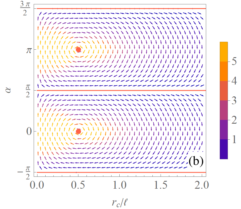
The points impact the dynamics of the dumbbell in the same way for any vortex flow. These points, indeed, form two straight lines () which separate the domain into two disconnected regions, so that the dynamics takes place in either of the stripes or depending on the initial orientation of the dumbbell [Fig. 7(a)]. As a consequence, the dumbbell never reverts its orientation with respect to the radial direction and the sign of remains constant during the time evolution, as was observed in Sect. III in the case of the Lamb–Oseen vortex.
Finally, a very general result can be deduced from Eqs. (10a) and (10b). These equations indeed display the same dependence on and and can be combined to yield
| (13) |
It follows that
| (14) |
is a constant of motion for all vortices. The implications of this result for the dynamics of the dumbbell depend on how the fluid angular velocity behaves as a function of .
IV.1 Decreasing fluid angular velocity
A wide class of single vortices, which includes the Lamb–Oseen vortex, the point vortex, and axisymmetric vortices with () Ravichandrana and Govindarajan 2015, has angular vorticity decreasing with increase in . We recall that in this case the set is empty. For such vortices, Eq. (14) indicates that the trajectories in the plane form a family of closed orbits around the fixed points and [see Fig. 7(a)]. Therefore, the variables and are periodic functions of time with same period. The orbits are parametrized by the initial conditions and .
The radial oscillation of the center of mass reverses its direction (inward or ouwards) when , that is when the connector is parallel or antiparallel to the radial direction. Hence, for a given orbit, the minimum and maximum values of , denoted as and , are the two roots of the equation
| (15) |
By using Eq. (15), it is thus possible to calculate the amplitude and the distance around which the oscillation takes place as and , respectively. The solid lines in Figs. 4(a,b) and 5(a,b) and the contour plot of in Fig. 6(b) have been obtained in this way. Since is a concave function of and vanishes as tends to either zero or infinity, both and diverge when either approaches or tends to zero or infinity. For such initial configurations, the centre of mass performs very wide oscillations, as was noted in Sect. III. Moreover, the solutions of Eq. (15) do not depend on and separately, but only on the ratio . Hence the functional dependence of and on and is independent of and, for fixed and , the values of and are proportional to (see Figs. 4 and 5). Figure 6(b) also shows that the dynamics becomes less and less sensitive to the initial orientation as is increased.
The correlation between the orientation of the dumbbell and the direction of its radial motion, shown in Fig. 2(b), can also be predicted from Eq. (10a). Indeed, if is decreasing, then the sign of is fixed at the beginning of the evolution (recall that during the motion the dumbbell never reverses its orientation with respect to the radial direction). Therefore, whether the radial motion is inward or outward is entirely determined by the sign of .
It ought be stressed that Eq. (14) is independent of . Therefore, all the properties of the dynamics that have been mentioned so far are independent of the form of the vortex, provided that decreases with increasing . In particular, the dependence of and on the initial configuration of the dumbbell [see the solid lines in Figs. 4(a,b) and 5(a,b) and the contour plot of in Fig. 6] is the same irrespective of the functional form of . What varies with the specific form of the vortex is the speed at which the orbits in the plane are covered, which in turn determines the evolution of the angle and ultimately the shape of the spirographic trajectories in physical space. Therefore, the behavior of which was shown in Figs. 4(c) and 5(c) is not generic but is specific to the Lamb–Oseen vortex. To explain this further, in Fig. 7(b) we show a vector plot of the field for the Lamb–Oseen vortex where the color of the arrows is a function of the magnitude of the vector field. Clearly, the orbits of the system are those described in Fig. 7(a), which are the same for any vortex with decreasing . However, the speed of the system along such orbits depends on the details of the Lamb–Oseen vortex. A different vortex would perform the same orbits but at a different speed. It would thus generate spirographic trajectories with same amplitude and at same radial distance, but of a different shape.
Finally, since the evolution of and is periodic, the right-hand side of Eq. (10c) is also periodic with same time period . As a consequence, the evolution of can be written as
| (16) |
where is a periodic function of period and is the average of the right-hand side of Eq. (10c) over a time period. In general, differs from , and therefore the rotational motion is not periodic. This explains the behavior observed in Sect. III, where the time evolution of was found to be the combination of a linear growth and a periodic oscillation of period superposed to it [see Figs. 2(d) and (e)].


IV.2 Rankine vortex
It was mentioned above that for the set to be non-empty, the fluid angular velocity must be a non-monotonic function of the radial distance. To explore how this additional set of fixed points may modify the dynamics of the dumbbell, we thus consider vortices such that is not strictly decreasing. We start with the Rankine vortex Saffman 1992; Wu et al. 2006, whose spatial structure is simple enough to allow an analytical study. The Rankine vortex indeed consists of an inner core of size which is in solid-body rotation and an outer region where the flow is potential [Fig. 7(c)]:
| (17) |
Compared to vortices with decreasing angular velocity, there exists a new set of fixed points in the plane. This corresponds to configurations in which both the beads lie in the solid-body-rotation core:
| (18) | ||||
| (19) |
The interior of obviously is neutrally stable. In contrast, a linear stability analysis shows that the boundary of is stable for and unstable for . The unstable (stable) portions of the boundary act as a repelling (attracting) set for the trajectories that start outside (see Fig. 8).
Three different regimes can be identified depending on the ratio [see the vector plots of the field in Fig. 8]:


- (i)
if , the fixed points and lie inside [Fig. 8(a)]. Therefore, if the system starts outside or on its repulsing boundary, it eventually ends up on the attracting boundary of . Periodic orbits are not possible in this case: either the dumbbell is in solid-body rotation from the very beginning or it ends up in solid-body rotation after a transient. Note that the motion towards the attracting set continues to take place along the curves described by Eq. (14), even though now the orbits are not performed in full.
- (ii)
if , the fixed points and lie outside [Fig. 8(b)]. Periodic orbits are now possible for initial conditions close to and . These periodic orbits are given by Eq. (14) and are therefore the same as for any vortex with decreasing angular velocity. What varies is the speed at which the orbits are performed.
- (iii)
if , the set is empty [see Fig. 8(c)]. The dumbbell is indeed too long compared to for both the beads to lie inside the solid-body-rotation core. In this case, the dynamics is qualitatively similar to that described in Sect.IV.1 and consists of periodic orbits around either or depending on the value of .
To show further how the existence of an attracting set modifies the dynamics, in Fig. 9 we compare the long-time spatial distribution of an ensembe of dumbbells in the Lamb–Oseen and Rankine vortices (see also Supplemental Movies 3 to 5 Lam; Ran; Ann). Naturally, this should only be regarded as a way to visualize the attracting set and not as a realistic simulation of an ensemble of dumbbells. The latter, indeed, would require accounting for mechanical and hydrodynamic interactions between dumbbells, which are instead disregarded here.


In the Lamb–Oseen vortex, the dumbbells spread around the vortex center while performing spirographic trajectories with different amplitudes and at different distances from the vortex center, and no pattern emerges in their spatial distribution (see Fig. 9(a) and Supplemental Movie 3 Lam). In the Rankine vortex, the dynamics is similar to that in the Lamb–Oseen vortex if (not shown). When the dumbbells that start entirely inside the disk perform a solid-body rotation, while those that have at least one bead outside the disk display a different behavior according to their length and initial configuration. If , all such dumbbells eventually end up performing a solid-body rotation in the annulus , the inner and outer radii of which are determined by the location of the boundary of at and , respectively. If , the dumbbells that have an initial configuration which is far from , are attracted inside the aforementioned annulus, whereas those that start in a configuration close to , perform spirographic trajectories. In this case, the long-time spatial distribution of the centers of mass consists of a core which is in solid-body rotation and an oscillating halo around the distance (see Fig. 9(b) and Supplemental Movie 4 Ran). It is interesting to note that, when , the boundary of in the plane acts as a transport barrier that prevents the centers of mass of the dumbbells from penetrating inside the disk from outside. Therefore, if the initial distribution of the dumbbells is such that for all them, then the disk remains empty at later times (see Supplemental Movie 5 Ann).
The study of the Rankine vortex reveals two main differences with the case of decreasing fluid angular velocity. First, the ratio is now an important parameter which discriminates between different dynamical regimes. Second, an attracting set emerges, which was absent in vortices with decreasing . Since the specific shape of this set plays a crucial role, the dynamics of the dumbbell in vortices with non-decreasing angular velocity does not enjoy the same degree of universality as in the case of a decreasing . To illustrate this further, we consider a two-dimensional version of the Sullivan vortex. This can no longer be solved analytically but has a smooth angular velocity.
IV.3 Two-dimensional Sullivan vortex
Sullivan Sullivan 1959 found an exact vortex solution of the three-dimensional Navier–Stokes equations with a two-cell spatial structure, i.e. with a region of reverse flow near to the axis of the vortex (see also Refs. Saffman 1992; Wu et al. 2006). The fluid angular velocity displays a maximum at a given distance from the vortex center [Fig. 7(c)]. This can be used to construct a stable vortex solution of the two-dimensional Euler equations with non-monotonic angular velocity. takes the form
| (20) |
where and the function is expressed as
| (21) |
The constant is chosen in such a way that the maximum of is at Vatistas 1998.
In each of the stripes and of the plane, the set of fixed points forms again a line that divides the stripe into two separate regions [Fig. 8(d)]. The line consists of an attracting and a repelling portion, and its shape varies with . The set now corresponds to those configurations in which one of the beads lies at while the other is at and . Two different behaviors can be observed in the plane [see the vector plot in Fig. 8(d)]. If the dumbbell starts sufficiently close to (, 0) or (, ), then it performs periodic orbits according to Eq. (14); otherwise it eventually ends up on the attracting portion of .
To visualize the dynamics and show how it is influenced by the presence of the set , we have again simulated the motion of the center of mass of an ensemble of dumbbells (see Supplemental Movie 6 Sul). For simplicity, in the simulations we have used an approximation of the Sullivan angular-velocity profile that was proposed by Wood and Brown Wood and Brown 2011: . The dumbbells whose initial conditions are close to () or () perform spirographic trajectories in an annulus around . Those that have an initial configuration far from () and () with () move away from (move towards) the vortex center and eventually end up performing solid-body rotation. Consequently, the long-time spatial distribution of the dumbbells in the Sullivan vortex consists of an annulus which is in solid-body rotation an oscillating halo around (see Fig. 9(c) and Supplemental Movie 6 Sul).
Thus, the example of the two-dimensional Sullivan vortex further demonstrates that if does not decrease with , the attracting set that emerges in the plane strongly impacts the dynamics of the dumbbell in a way that is specific to the particular form of the vortex. Different dynamical regimes may in principle be generated by modifying the funcional dependence of on .
V Summary and concluding remarks
This study investigates the motion of particles in a vortex flow by going beyond the point-particle approximation. It thus aims to be a step in the direction of a better understanding of the dynamics of extended objects in a flow field. In the case of a rigid dumbbell, the simplicity of the system allows a detailed analysis of the motion and of its dependence on the properties of the vortex.
The main result is that, in the class of two-dimensional steady vortices with angular velocity decreasing as a function of the radial distance, the center of mass of a rigid dumbbell performs spirographic trajectories around the vortex center. The qualitative features of the dynamics do not depend on the details of the vortex. For instance, the amplitude of the radial oscillation and the distance around which the oscillation is performed are fully independent of the functional form of the vortex. The situation changes when the fluid angular velocity is not strictly monotonic. An attracting set emerges in the configuration space, and this impacts the dynamics in a way that depends on the details of the vortex.
The analysis is restricted to steady vortices, but several results also apply to time-dependent vortices. In particular, the quantity remains a constant of motion even for a time-dependent vortex and the orbits in the plane are unchanged: only the way these orbits are covered varies according to the temporal evolution of the fluid angular velocity. Two-dimensional turbulent flows forced at large scales are characterized by large long-lived vortices in the vicinity of which straining is weak. A dumbbell would typically remain in a given vorticity-dominated region for a long time, during which the quantity would remain constant. It would be interesting to explore the consequences of this conserved quantity for the dynamics of dumbbells in two-dimensional turbulence.
The study also disregards Brownian fluctuations. However, an inspection of the vector plots in Figs. 7 and 8 shows that, for most initial configurations, Brownian fluctuations would only cause small perturbations of the spirographic dynamics. In contrast, inertial effects may have a strong impact. If the inertia of the beads is not negligible, the dumbbell is likely to acquire a nonzero mean radial velocity resulting in its ejection or entrapment depending on the ratio between the bead and fluid density Raju and Meiburg 1997. Nevertheless, we have seen that the instantaneous radial velocity of the dumbbell depends on its orientation. It would therefore be interesting to study whether the orientation dynamics of the dumbbell speeds up or slows down its ejection or entrapment.
Finally, in a dumbbell only the two beads interact with the fluid, and hence the drag force is concentrated at the ends of the object. Nevertheless, based on the above analysis of the spirographic dynamics, we expect that a rigid fiber would perform a qualitatively similar motion, even though the effects of the hydrodynamic interactions between the segments of the fiber remain to be understood.
Acknowledgements.
The authors are grateful to Giorgio Krstulovic and Jason R. Picardo for helpful discussions. SRY acknowledges the financial support from the CNRS through the 80 Prime program. RG acknowledges support of the Department of Atomic Energy, Government of India, under project no. RTI4001. DV acknowledges the support of the Indo–French Center for Applied Mathematics (IFCAM).*
Appendix A
Recall that, in polar coordinates, the orthogonal bases at the positions of the beads and of the centre of mass are denoted as and , respectively. These obey the relationships
| (22) |
whence
| (23) |
In addition
| (24) |
By using the definition of the velocity in Eqs. (6) and (7) as well as Eq. (23) and the second of Eqs. (24), we find
| (25) |
Thus, Eq. (5a) yields
| (26) |
which is Eq. (10a). To derive the evolution equation for , we first note that
| (27) |
Then, Eq. (5b) yields
| (28) |
By using Eqs. (26) and (28) in Eq. (27), we find
| (29) |
which gives Eq. (10b). The -component of Eq. (5a) may now be used to derive an evolution equation for :
| (30) |
Note that Eq. (12) implies
| (31) |
where
| (32) |
is such that . By using Eqs. (31), we can rewrite Eq. (5a) as
| (33) |
We thus find
| (34) |
Finally, inserting the latter expression in Eq. (30) yields
| (35) |
and hence Eq. (10c).
References
- Lázaro and Lasheras (1989) B. J. Lázaro and J. C. Lasheras, Particle dispersion in a turbulent, plane, free shear layer, Phys. Fluids A 1, 1035 (1989).
- Raju and Meiburg (1997) N. Raju and E. Meiburg, Dynamics of small, spherical particles in vortical and stagnation point flow fields, Phys. Fluids 9, 299 (1997).
- Candelier et al. (2004) F. Candelier, J. R. Angilella, , and M. Souhar, On the effect of the Boussinesq–Basset force on the radial migration of a Stokes particle in a vortex, Phys. Fluids 16, 1765 (2004).
- Goater and Lawrence (2004) A. Goater and G. A. Lawrence, Dispersion of heavy particles in an isolated pancake-like vortex, J. Environ. Eng. Sci. 3, 403 (2004).
- Ravichandrana and Govindarajan (2015) S. Ravichandrana and R. Govindarajan, Caustics and clustering in the vicinity of a vortex, Phys. Fluids 27, 033305 (2015).
- Deepu et al. (2017) P. Deepu, S. Ravichandran, and R. Govindarajan, Caustics-induced coalescence of small droplets near a vortex, Phys. Rev. Fluids 2, 024305 (2017).
- Ruetsch and Meiburg (1993) G. R. Ruetsch and E. Meiburg, On the motion of small spherical bubbles in two-dimensional vertical flows, Phys. Fluids A 5, 2326 (1993).
- Sokolov and Aranson (2016) A. Sokolov and I. S. Aranson, Rapid expulsion of microswimmers by a vortical flow, Nat. Commun. 7, 11114 (2016).
- Tarama et al. (2014) M. Tarama, A. M. Menzel, and H. Löwen, Deformable microswimmer in a swirl: Capturing and scattering dynamics, Phys. Rev. E 90, 032907 (2014).
- Arguedas-Leiva and Wilczek (2020) J.-A. Arguedas-Leiva and M. Wilczek, Microswimmers in an axisymmetric vortex flow, New J. Phys. 22, 053051 (2020).
- Berman et al. (2021) S. A. Berman, J. Buggeln, D. A. Brantley, K. A. Mitchell, and T. H. Solomon, Transport barriers to self-propelled particles in fluid flows, Phys. Rev. Fluids 6, L012501 (2021).
- Guedda et al. (2021) M. Guedda, J. Chaiboub, M. Benlahsen, and C. Misbah, Exact trajectory solutions of a spherical microswimmer under flow and external fields, Phys. Rev. Fluids 6, 074102 (2021).
- Graham (2018) M. D. Graham, Microhydrodynamics, Brownian Motion, and Complex Fluids (Cambridge University Press, Cambridge, UK, 2018).
- Besant (1890) W. H. Besant, Notes on Roulettes and Glissettes, 2nd ed. (Deighton, Bell & Co., Cambridge, England, 1890).
- Piva and Martino (2009) M. F. Piva and G. R. Martino, A rigid dumbbell settling under gravity in a periodic flow field, J. Phys. A: Math. Theor. 42, 025501 (2009).
- (16) See https://youtu.be/zswLMOvTaqY for the movie showing the dynamics of a dumbbell of length for and in the Lamb–Oseen vortex with and . The beads in the movie are coloured differently only for the visualization purposes.
- (17) See https://youtu.be/IGt0qc5_Js0 for the movie showing the dynamics of a dumbbell of length for and in the Lamb–Oseen vortex with and . The beads in the movie are coloured differently only for the visualization purposes.
- Cencini et al. (2009) M. Cencini, F. Cecconi, and A. Vulpiani, Chaos: From Simple Models to Complex Systems (World Scientific, Singapore, 2009).
- Saffman (1992) P. G. Saffman, Vortex Dynamics (Cambridge University Press, Cambridge, UK, 1992).
- Wu et al. (2006) J.-Z. Wu, H.-Y. Ma, and M.-D. Zhou, Vorticity and Vortex Dynamics (Springer-Verlag, Berlin Heidelberg, 2006).
- (21) See https://youtu.be/UClfE_Ec25k for the movie showing the dynamics of the centers of mass of non-interacting dumbbells of length in the Lamb–Oseen vortex with and . At , the centers of mass are distributed uniformly over a disc of radius 1.6.
- (22) See https://www.youtube.com/watch?v=_8LtHk58E_g&t=10s for the movie showing the dynamics of the centers of mass of non-interacting dumbbells of length in the Rankine vortex with and . At , the centers of mass are distributed uniformly over a disc of radius 1.6.
- (23) See https://youtu.be/G9xDsvV6vcA for the movie showing the dynamics of the centers of mass of non-interacting dumbbells of length in the Rankine vortex with and . At , the centers of mass are distributed uniformly over an annulus of inner and outer radii 0.6 and 1.6, respectively.
- Sullivan (1959) R. D. Sullivan, A two-cell vortex solution of the Navier–Stokes equations, J. Aerosp. Sci. 26, 767 (1959).
- Vatistas (1998) G. H. Vatistas, New model for intense self-similar vortices, J. Prop. Power 14, 462 (1998).
- (26) See https://www.youtube.com/watch?v=KXHC9wUPvXc for the movie showing the dynamics of the centers of mass of non-interacting dumbbells of length in the Sullivan vortex with and . At , the centers of mass are distributed uniformly over a disc of radius 1.5.
- Wood and Brown (2011) V. T. Wood and R. A. Brown, Simulated tornadic vortex signatures of tornado-like vortices having one- and two-celled structures, J. Appl. Meteorol. Climatol. 50, 2338 (2011).