Uniformly accurate integrators for Klein–Gordon–Schrödinger systems from the classical to non-relativistic limit regime

María Cabrera Calvo Address: Laboratoire Jacques-Louis-Lions, Sorbonne Université, France Email: maria.cabrera_calvo@sorbonne-universite.fr

Abstract

In this paper we present a novel class of asymptotic consistent exponential-type integrators for Klein–Gordon–Schrödinger systems that capture all regimes from the slowly varying classical regime up to the highly oscillatory non-relativistic limit regime. We achieve convergence of order one and two that is uniform in $c$ without any time step size restrictions. In particular, we establish an explicit relation between gain in negative powers of the potentially large parameter $c$ in the error constant and loss in derivative.

Keywords:

Klein–Gordon–Schrödinger, highly oscillatory integral, asymptotic consistency

1 Introduction

We consider the Klein–Gordon–Schrödinger system

	$\displaystyle$	$\displaystyle c^{-2}\partial_{tt}z(t,x)-\Delta z(t,x)+c^{2}z(t,x)=\|\psi(t,x)\|^{2},$		(1)
		$\displaystyle i\partial_{t}\psi(t,x)+\frac{1}{2}\Delta\psi(t,x)+\psi(t,x)z(t,x)=0,$		(1)

given by a Klein–Gordon equation coupled nonlinearly with a classical Schrödinger equation. This setting arises in quantum field theory, representing the dynamics of the interaction between a complex-valued scalar nucleon field $\psi:\mathbb{R}\times\mathbb{R}^{d}\to\mathbb{C}$ with a neutral real-valued scalar meson field $z:\mathbb{R}\times\mathbb{R}^{d}\to\mathbb{R}$ . For existence and uniqueness of global smooth solutions see [9], [10], [11].

The parameter $c$ , proportional to the speed of light, plays a very important role in the behaviour of the solution and gives rise to two different regimes. We distinguish between the so-called relativistic regime, where $c=1$ , and the non-relativistic regime with $c\gg 1$ . The former regime is well studied numerically, for instance see [2], as its solution is slowly varying. The non-relativistic, on the other hand, brings in a significant additional challenge in terms of its numerical treatment, given the highly oscillatory nature of its solution. It causes classical numerical methods to collapse, as they fail to capture the rapid oscillations, leading to large errors or, in turn, severe time step size restrictions and thus very intense computational efforts. This is even the case for Gautschy-type methods (see [1], [13]), which were specifically designed to numerically solve highly oscillatory problems. Splitting methods fail to deal with these rapid oscillations in a similar way, see for instance [7] for their analysis in the context of Schrödinger equations.

In [3], an unconditionally stable method was developed, based on a multi-scale expansion technique, that achieves uniform linear convergence in time, for sufficiently smooth solutions. Quadratic convergence was achieved in this setting, yet only in the case where either $c=\mathcal{O}(1)$ or $c\tau\geq 1$ .

In [4] an approach was presented that succeeded to capture all regimes in $c$ , providing error bounds that were independent of this parameter and without requiring any step size restrictions. This was done by means of the introduction of the so-called twisted variables, that were already well known both in physics as "interaction picture", and in the study of partial differential equations at low regularity. The main idea therein was to explicitly filter out the highly oscillatory phases, approximate the slowly varying parts, which does not produce dependency on $c$ in the error constants, and integrate the interacting highly oscillatory phases exactly. In addition, this approach achieves asymptotic consistency, meaning that it preserves the NLS limit on the discrete level.

In comparison to [4], we propose a novel class of exponential-type integrators that equally manages to capture all regimes of $c$ , without any time step size restrictions, and is asymptotically consistent. We introduce a new construction, exploiting the structure of the leading differential operators $\frac{1}{2}\Delta$ and $c\langle\nabla\rangle_{c}$ , which allows us to establish an explicit relation between a gain of negative powers of the potentially very large parameter $c$ in the error constant versus a loss of derivative. In other words, a gain in accuracy, in the non-relativistic regime, in exchange of a loss in derivative. In addition to this, in the first order scheme, we require one derivative less in the Klein–Gordon part than pre-existing methods up to our knowledge. We achieve this by employing techniques introduced in [5] in the context of the Klein–Gordon equation. This recent work couples the ideas of low regularity (in space) approximation presented in [18] in the context of an abstract class of of evolution equations, with the idea of uniform accuracy achieved in [4].

The underlying strategy is the expansion of suitable filtered functions that allows the embedding of the full spectrum of oscillations into the numerical scheme. Here, the commutator structure of the leading operator $\frac{1}{2}\Delta$ and is studied (see Lemma 3.1), as it plays a crucial role in the achievement of low regularity approximations that do not produce powers of $c$ in our error estimates. In addition to this, we study the asymptotic behaviour of the leading operator $c\langle\nabla\rangle_{c}$ in order to resolve the nonlinear frequency interaction caused by the coupled nature of this system.

In the present setting, however, the fact that the equations are coupled non-linearly supposes an additional challenge. It makes the analysis much more involved, since one has to consider the non-linear interaction of highly oscillatory parts. This rises the need of new, adapted techniques.

Outline of the paper. We begin by expressing (1) as a first order system in time in Section 2. In Section 3 we motivate the new first order scheme and it’s second order counterpart will be derived in Section 4. We prove their uniform convergence in Theorems 3.6 and 4.10, respectively. In Section 5 we briefly present the limit system, show that, as $c\to\infty$ formally, we recover the solution to the limit system. Finally, numerical experiments are presented in Section 6, confirming our theoretical results.

Notation. For reasons regarding ease of implementation and clarity of presentation, we impose periodic boundary conditions, i.e. $x\in\mathbb{T}^{d}$ . However, we note that nor the construction nor the analysis of our scheme depends on any Fourier expansion techniques, and thus can be generalised to bounded domains $x\in\Omega\subset\mathbb{R}^{d}$ equipped with suitable boundary conditions, as well as the full space $x\in\mathbb{R}^{d}$ . For simplicity, we may occasionally make use of $\mathcal{O}$ -notation exclusively in the context of constants independent of $c$ . For the sake of simplifying future notation, we define the $\varphi_{1}$ -function as

\displaystyle\varphi_{1}(\xi)=\frac{e^{\xi}-1}{\xi},\quad\xi\in\mathbb{C}.

(2)

We also note

\displaystyle\varphi_{1}(\xi)=1+\mathcal{O}(\xi).

(3)

We refer to [16] for details on this family of functions. In the following we fix $r>\frac{d}{2}$ and we denote by $\|.\|_{r}$ the standard $H^{r}=H^{r}(\mathbb{T}^{d})$ Sobolev norm, where, for this choice of $r$ , the following well-known bilinear estimate holds

\|fg\|_{r}\leq C_{r,d}\|f\|_{r}\|g\|_{r},

for some constant $C_{r,d}>0$ independent of $f$ and $g$ .

2 Formulation as a first order system

We start by defining the following differential operator that will simplify our notation significantly. For a given $c>0$ we define the following operator

\displaystyle c\langle\nabla\rangle_{c}=c\sqrt{c^{2}-\Delta}.

One can verify that this differential operator is well-defined, as its corresponding Fourier multiplier has the form $(\langle\nabla\rangle_{c})_{k}=\sqrt{k^{2}+c^{2}}$ . We may now rewrite (1) as a first order system in time (see [17]). Setting

\displaystyle u=z-ic^{-1}\langle\nabla\rangle_{c}^{-1}\partial_{t}z,\quad v=z-ic^{-1}\langle\nabla\rangle_{c}^{-1}\partial_{t}\overline{z},

(4)

a simple calculation shows that $z=\frac{1}{2}(u+v)$ . Furthermore, if we assume that $z(t,x)\in\mathbb{R}$ , we have

\displaystyle z=\frac{1}{2}(u+\overline{u}).

(5)

In the following we will restrict our attention to this case purely for the purpose of presenting our main ideas as clearly as possible. Note, however, that this does not impose any significant restriction. Having said this, a short calculation shows that the corresponding first order system in $(u,\psi)$ reads

		$\displaystyle i\partial_{t}u+c\langle\nabla\rangle_{c}u-c\langle\nabla\rangle_{c}^{-1}\|\psi\|^{2}=0,$		$\displaystyle u(0)=z(0)-ic^{-1}\langle\nabla\rangle_{c}^{-1}\partial_{t}z(0),$		(6)
		$\displaystyle i\partial_{t}\psi+\frac{1}{2}\Delta\psi+\frac{1}{2}\psi(u+\overline{u})=0,$		$\displaystyle\psi(0)=\psi_{0}.$		(7)

3 A first order integrator

In this section we proceed to give a detailed derivation of the numerical scheme for $u^{n+1}\approx u(t_{n+1})$ with $t_{n+1}=t_{n}+\tau$ , followed by a less detailed derivation of the numerical scheme for $\psi^{n+1}\approx\psi(t_{n+1})$ that employs analogous ideas. Duhamel’s formula for (6) reads

u(t_{n}+\tau)=e^{i\tau c\langle\nabla\rangle_{c}}u(t_{n})-ic\langle\nabla\rangle_{c}^{-1}e^{i\tau c\langle\nabla\rangle_{c}}\int_{0}^{\tau}e^{-isc\langle\nabla\rangle_{c}}|\psi(t_{n}+s)|^{2}ds.

Iterating Duhamel’s formula for (7) leads to

\displaystyle u(t_{n}+\tau)=e^{i\tau c\langle\nabla\rangle_{c}}u(t_{n})-ic\langle\nabla\rangle_{c}^{-1}e^{i\tau c\langle\nabla\rangle_{c}}\int_{0}^{\tau}e^{-isc\langle\nabla\rangle_{c}}|e^{i\frac{1}{2}s\Delta}\psi(t_{n})|^{2}ds+\mathcal{R}_{1},

(8)

where $\mathcal{R}_{1}$ fulfills a bound of the form

$\displaystyle\\|\mathcal{R}_{1}\\|_{r}$	$\displaystyle\leq\bigg\\|ic\langle\nabla\rangle_{c}^{-1}e^{i\tau c\langle\nabla\rangle_{c}}\int_{0}^{\tau}e^{-isc\langle\nabla\rangle_{c}}\big(e^{-i\frac{1}{2}s\Delta}\overline{\psi(t_{n})}\big)\mathcal{I}_{\psi}(s)\,ds\bigg\\|_{r}$	(9)
	$\displaystyle+\bigg\\|ic\langle\nabla\rangle_{c}^{-1}e^{i\tau c\langle\nabla\rangle_{c}}\int_{0}^{\tau}e^{-isc\langle\nabla\rangle_{c}}\big(e^{i\frac{1}{2}s\Delta}{\psi(t_{n})}\big)\mathcal{I}_{\psi}(s)\,ds\bigg\\|_{r}$
	$\displaystyle+\bigg\\|ic\langle\nabla\rangle_{c}^{-1}e^{i\tau c\langle\nabla\rangle_{c}}\int_{0}^{\tau}e^{-isc\langle\nabla\rangle_{c}}\big\|\mathcal{I}_{\psi}(s)\big\|^{2}ds\bigg\\|_{r}$
	$\displaystyle\leq\tau^{2}K\big(\sup_{0\leq\xi\leq\tau}\\|\psi(t_{n}+\xi)\\|_{r}\big),$

where

\displaystyle\mathcal{I}_{\psi}(s)=\frac{i}{2}e^{i\frac{1}{2}s\Delta}\int_{0}^{s}e^{-i\frac{1}{2}\sigma\Delta}\psi(t_{n}+\sigma)\big(u(t_{n}+\sigma)+\overline{u(t_{n}+\sigma)}\big)d\sigma,

(10)

thanks to the following remarks

\displaystyle\|c\langle\nabla\rangle_{c}^{-1}\|_{r}\leq 1,\quad\|e^{itc\langle\nabla\rangle_{c}}\|_{r}=1,\quad\|e^{it\Delta}\|_{r}=1\,\quad\forall t\in\mathbb{R}.

(11)

It is left to approximate the present oscillatory integral in a suitable way and, to this end, we introduce the following crucial commutator term, which will appear in our local error estimates.

Definition 3.1.

For a function $H(v_{1},\dots,v_{n})$ , $n\geq 1$ , and a linear operator $L:H^{r}\to H^{r}$ we define the following commutator type term

\displaystyle\mathcal{C}[H,L](v_{1},\dots,v_{n})=-L(H(v_{1},\dots,v_{n}))+\sum_{i=1}^{n}D_{i}H(v_{1},\dots,v_{n})\cdot Lv_{i},

where $D_{i}H$ stands for the partial derivative of H with respect to the variable $v_{i}$ . Furthermore, we set

\mathcal{C}^{2}[H,L](v_{1},\dots,v_{n})=\mathcal{C}[\mathcal{C}[H,L],L](v_{1},\dots,v_{n})

and

f_{\text{quad}}(v,w)=vw.

We now establish the necessary bounds for these commutator type terms.

Lemma 3.1.

We have that

		$\displaystyle\\|\mathcal{C}[f_{\text{quad}}(\cdot,\cdot),\Delta](v,w)\\|_{r}\leq K_{1}\\|v\\|_{r+1}\\|w\\|_{r+1},$
		$\displaystyle\\|\mathcal{C}^{2}[f_{\text{quad}}(\cdot,\cdot),\Delta](v,w)\\|_{r}\leq K_{2}\\|v\\|_{r+2}\\|w\\|_{r+2}$

for some $K_{1},K_{2}>0$ .

Proof.

We will show the first assertion in detail, the second assertion can be proven iterating this argument. By definition,

\displaystyle\mathcal{C}[f_{\text{quad}}(\cdot,\cdot),\Delta](v,w)=-\Delta(vw)+w\Delta v+v\Delta w.

The assertion follows by the product rule of the Laplacian

\Delta(vw)=v\Delta w+2\nabla v\cdot\nabla w+w\Delta v.

∎

We now aim to capture the oscillatory integral in (8) in a way that does not trigger dependency on $c$ in the error terms and allows a low regularity approximation. The technique is captured in the following lemma.

Lemma 3.2 (First order approximation of the integral in (8)).

It holds that

\displaystyle\int_{0}^{\tau}e^{-isc\langle\nabla\rangle_{c}}|e^{i\frac{1}{2}s\Delta}v|^{2}ds=\tau\overline{v}\varphi_{1}(i\tau(\Delta-c^{2}))v+\mathcal{O}\big(\tau^{2}(\mathcal{C}[f_{\text{quad}}(\cdot,\cdot),\Delta](v,v)+c^{-2\alpha}\Delta^{1+\alpha}v)\big).

Proof.

We introduce the following filtered function defined by

\displaystyle\mathcal{N}(s,s_{1},\Delta,v):=e^{i\frac{1}{2}s_{1}\Delta}\big(e^{-i\frac{1}{2}s_{1}\Delta}e^{is\Delta}v\big)\big(e^{-i\frac{1}{2}s_{1}\Delta}\overline{v}\big).

(12)

Then, the integral reads

\int_{0}^{\tau}e^{-isc\langle\nabla\rangle_{c}}|e^{i\frac{1}{2}s\Delta}v|^{2}ds=\int_{0}^{\tau}e^{-isc\langle\nabla\rangle_{c}}e^{-i\frac{1}{2}s\Delta}\mathcal{N}(s,s,\Delta,v)ds.

At this point one needs to first tackle the interactions between the differential operators $c\langle\nabla\rangle_{c}$ and $\frac{1}{2}\Delta$ . Note that, as it can be shown via fractional Taylor series expansion of the function $x\to c^{2}\sqrt{c^{2}+x^{2}}$ , it holds

\displaystyle c\langle\nabla\rangle_{c}=c^{2}-\tfrac{1}{2}\Delta+\mathcal{O}\big(\tfrac{\Delta^{1+\alpha}}{c^{2\alpha}}\big),\quad 0\leq\alpha\leq 1,

(13)

and thus,

\int_{0}^{\tau}e^{-isc\langle\nabla\rangle_{c}}e^{-i\frac{1}{2}s\Delta}\mathcal{N}(s,s,\Delta,v)ds=\int_{0}^{\tau}e^{-isc^{2}}\mathcal{N}(s,s,\Delta,v)ds+\mathcal{R}_{1},

where, using (13), we see that we may bound $\mathcal{R}_{1}$ by

\displaystyle\|\mathcal{R}_{1}\|_{r}\leq c^{-2\alpha}K(\|v\|_{r+2(1+\alpha)}),\quad 0\leq\alpha\leq 1,

(14)

for some $K^{\prime}>0$ independent of $c$ .

On the other hand, Taylor series expansion gives the following approximation

\mathcal{N}(s,s_{1},\Delta,v)=\mathcal{N}(s,0,\Delta,v)+\int_{0}^{s}\partial_{s_{1}}\mathcal{N}(s,s_{1},\Delta,v)ds_{1}.

Thus, plugging in this expansion and then integrating exactly we obtain

	$\displaystyle\int_{0}^{\tau}e^{-isc\langle\nabla\rangle_{c}}e^{i\frac{1}{2}s\Delta}\mathcal{N}(s,s,\Delta,v)ds$	$\displaystyle=\int_{0}^{\tau}e^{-isc^{2}}\mathcal{N}(s,0,\Delta,v)ds+\mathcal{R}_{1}$
		$\displaystyle=\int_{0}^{\tau}e^{-isc^{2}}\big(e^{is\Delta}{v}\big)\overline{v}ds+\mathcal{R}_{1}+\mathcal{R}_{2}$
		$\displaystyle=\tau\overline{v}\varphi_{1}(i\tau(\Delta-c^{2}))v+\mathcal{R}_{1}+\mathcal{R}_{2},$

where $\mathcal{R}_{2}$ can be bounded as follows. By (11) and the remark

\displaystyle\partial_{s_{1}}\mathcal{N}(s,s_{1},\Delta,v)_{|s_{1}=s}=e^{i\frac{1}{2}s_{1}\Delta}\mathcal{C}[f_{\text{quad}}(\cdot,\cdot),-i\tfrac{1}{2}\Delta](e^{-i\frac{1}{2}s_{1}\Delta}e^{is\Delta}v,e^{-i\frac{1}{2}s_{1}\Delta}\overline{v}).

it holds

\displaystyle\|\mathcal{R}_{2}\|_{r}\leq\bigg\|\int_{0}^{\tau}e^{-isc\langle\nabla\rangle_{c}}e^{i\frac{1}{2}s\Delta}\bigg(\int_{0}^{s}\partial_{s_{1}}\mathcal{N}(s,s_{1},\Delta,v)ds_{1}\bigg)ds\bigg\|_{r}\leq\tau^{2}K\big(\mathcal{C}[f_{\text{quad}}(\cdot,\cdot),i\tfrac{1}{2}\Delta](v,\overline{v})\big).

∎

The expansion (8) together with Lemma 3.2 lead to the following first order uniformly accurate integrator

\displaystyle u^{n+1}=e^{i\tau c\langle\nabla\rangle_{c}}u^{n}-i\tau c\langle\nabla\rangle_{c}^{-1}e^{i\tau c\langle\nabla\rangle_{c}}\overline{\psi^{n}}\varphi_{1}(i\tau(\Delta-c^{2}))\psi^{n}.

(15)

Finally, given $u^{n+1}$ by (15), one can very easily find $z^{n+1}$ , via (5),

z^{n+1}=\frac{1}{2}\big(u^{n+1}+\overline{u^{n+1}}\big).

Now we proceed as follows for $\psi^{n+1}$ . Duhamel’s formula for (7) reads

\psi(t_{n}+\tau)=e^{i\frac{1}{2}\tau\Delta}\psi(t_{n})+i\frac{1}{2}e^{i\frac{1}{2}\tau\Delta}\int_{0}^{\tau}e^{-i\frac{1}{2}s\Delta}\psi(t_{n}+s)\big(u(t_{n}+s)+\overline{u(t_{n}+s)}\big)ds.

Iterating Duhamel’s formula for (6) and (7) respectively leads to

\displaystyle\psi(t_{n}+\tau)=e^{i\frac{1}{2}\tau\Delta}\psi(t_{n})+\frac{i}{2}e^{i\frac{1}{2}\tau\Delta}\int_{0}^{\tau}e^{-i\frac{1}{2}s\Delta}\big(e^{i\frac{1}{2}s\Delta}\psi(t_{n})\big)\big(e^{isc\langle\nabla\rangle_{c}}u(t_{n})+e^{-isc\langle\nabla\rangle_{c}}\overline{u(t_{n})}\big)ds+\mathcal{R}_{2},

(16)

where $\mathcal{R}_{2}$ fulfills the bound

\displaystyle\|\mathcal{R}_{2}\|_{r}\leq\|\mathcal{R}_{2,1}\|_{r}+\|\mathcal{R}_{2,2}\|_{r},

with

\displaystyle\mathcal{R}_{2,1}=\frac{i}{2}e^{i\frac{1}{2}\tau\Delta}\int_{0}^{\tau}e^{-i\frac{1}{2}s\Delta}\mathcal{I}_{\psi}(s)\big(e^{isc\langle\nabla\rangle_{c}}u(t_{n})+e^{-isc\langle\nabla\rangle_{c}}\overline{u(t_{n})}\big)ds,

with $\mathcal{I}_{\psi}$ given by (10) and

\displaystyle\mathcal{R}_{2,2}=\frac{i}{2}e^{i\frac{1}{2}\tau\Delta}\int_{0}^{\tau}e^{-i\frac{1}{2}s\Delta}\big(e^{i\frac{1}{2}s\Delta}\psi(t_{n})\big)\big(\mathcal{I}_{u}(s)+\overline{\mathcal{I}_{u}(s)}\big)ds,

\displaystyle\mathcal{I}_{u}(s)=ic\langle\nabla\rangle_{c}^{-1}e^{isc\langle\nabla\rangle_{c}}\int_{0}^{s}e^{-i\sigma c\langle\nabla\rangle_{c}}|\psi(t_{n}+\sigma)|^{2}d\sigma.

(17)

Thus, we conclude by (11) that

\displaystyle\|\mathcal{R}_{2}\|_{r}\leq\tau^{2}K\big(\sup_{t_{n}\leq t\leq t_{n+1}}\|u(t)\|_{r},\sup_{t_{n}\leq t\leq t_{n+1}}\|\psi(t)\|_{r}\big).

(18)

It is left to approximate the highly oscillatory integral in (16) and to this end we proceed analogously as in Lemma 3.2.

Lemma 3.3 (First order approximation of the integral in (16)).

It holds that

	$\displaystyle\int_{0}^{\tau}e^{-i\frac{1}{2}s\Delta}$	$\displaystyle\big(e^{i\frac{1}{2}s\Delta}v\big)\big(e^{isc\langle\nabla\rangle_{c}}w+e^{-isc\langle\nabla\rangle_{c}}\overline{w}\big)ds$
		$\displaystyle=\tau v\big(\varphi_{1}(i\tau(c\langle\nabla\rangle_{c}-\tfrac{1}{2}\Delta))w+\varphi_{1}(-i\tau(c\langle\nabla\rangle_{c}+\tfrac{1}{2}\Delta))\overline{w}\big)+\mathcal{O}(\tau^{2}\mathcal{C}[f_{\text{quad}}(\cdot,\cdot),i\Delta](v,w)).$

Proof.

We define the following filtered functions

\mathcal{N}(s,s_{1},\Delta,v,w)=e^{-i\frac{1}{2}s_{1}\Delta}\big(e^{i\frac{1}{2}s_{1}\Delta}v)(e^{i\frac{1}{2}s_{1}\Delta}e^{-i\frac{1}{2}s\Delta}(e^{isc\langle\nabla\rangle_{c}}w+e^{-isc\langle\nabla\rangle_{c}}\overline{w})\big).

Taylor series expansion around the point $s_{1}=0$ yields the following first order approximation

	$\displaystyle\int_{0}^{\tau}e^{-i\frac{1}{2}s\Delta}\big(e^{i\frac{1}{2}s\Delta}v\big)$	$\displaystyle\big(e^{isc\langle\nabla\rangle_{c}}w+e^{-isc\langle\nabla\rangle_{c}}\overline{w}\big)ds$
		$\displaystyle=\int_{0}^{\tau}\mathcal{N}(s,s,\Delta,v,w)ds=\int_{0}^{\tau}\mathcal{N}(s,0,\Delta,v,w)ds+\mathcal{R}$
		$\displaystyle={\tau v\big(\varphi_{1}(i\tau(c\langle\nabla\rangle_{c}-\tfrac{1}{2}\Delta))w+\varphi_{1}(-i\tau(c\langle\nabla\rangle_{c}+\tfrac{1}{2}\Delta))\overline{w}\big)}+\mathcal{R}.$

Once again we find a bound for $\mathcal{R}$ thanks to the observation

\partial_{s_{1}}\mathcal{N}(s,s_{1},\Delta,v,w)=e^{-i\frac{1}{2}s_{1}\Delta}\mathcal{C}[f_{\text{quad}}(\cdot,\cdot),i\tfrac{1}{2}\Delta](e^{i\frac{1}{2}s_{1}\Delta}v,e^{i\frac{1}{2}s_{1}\Delta}(e^{is_{1}c\langle\nabla\rangle_{c}}w+e^{-is_{1}c\langle\nabla\rangle_{c}}\overline{w})),

thus

\|\mathcal{R}\|_{r}\leq\tau^{2}K\big(\mathcal{C}[f_{\text{quad}}(\cdot,\cdot),i\tfrac{1}{2}\Delta](v,w)\big).

∎

Plugging our findings from Lemmata 3.2 and 3.3 into the expansion (16) motivates the following scheme for $\psi^{n+1}$ .

\displaystyle\psi^{n+1}=e^{i\frac{1}{2}\tau\Delta}\psi^{n}+\tau\frac{i}{2}e^{i\frac{1}{2}\tau\Delta}\psi^{n}\big(\varphi_{1}(i\tau(c\langle\nabla\rangle_{c}-\tfrac{1}{2}\Delta))u^{n}+\varphi_{1}(-i\tau(c\langle\nabla\rangle_{c}+\tfrac{1}{2}\Delta))\overline{u^{n}}\big).

(19)

In the sections that follow we aim to carry out the error analysis of the scheme in $(u^{n},\psi^{n})$ given by (15) and (19). Before we begin we denote by $\varphi^{t}_{K}$ , $\varphi^{t}_{S}$ the exact flows of (6) and (7) respectively and by $\Phi^{t}_{K}$ , $\Phi^{t}_{S}$ the numerical flows corresponding to (15) and (19) respectively, such that in particular it holds

u(t_{n+1})=\varphi^{\tau}_{K}(u(t_{n}),\psi(t_{n})),\,\psi(t_{n+1})=\varphi^{\tau}_{S}(u(t_{n}),\psi(t_{n})),\quad u^{n+1}=\Phi^{\tau}_{K}(u^{n},\psi^{n}),\,\psi^{n+1}=\Phi^{\tau}_{S}(u^{n},\psi^{n}).

3.1 Local error analysis

Lemma 3.4.

Fix $r>\frac{d}{2}$ . The local error given by the differences $\varphi^{\tau}_{K}(u(t_{n}),\psi(t_{n}))-\Phi^{\tau}_{K}(u(t_{n}),\psi(t_{n}))$ and $\varphi^{\tau}_{S}(u(t_{n}),\psi(t_{n}))-\Phi^{\tau}_{S}(u(t_{n}),\psi(t_{n}))$ satisfies

\varphi^{\tau}_{K}(u(t_{n}),\psi(t_{n}))-\Phi^{\tau}_{K}(u(t_{n}),\psi(t_{n}))=\mathcal{O}(\tau^{2}(\mathcal{C}[f_{\text{quad}}(\cdot,\cdot),i\tfrac{1}{2}\Delta]+c^{-2\alpha}\Delta^{1+\alpha}))(\psi(t_{n}),\overline{\psi(t_{n})}))

and

\varphi^{\tau}_{S}(u(t_{n}),\psi(t_{n}))-\Phi^{\tau}_{S}(u(t_{n}),\psi(t_{n}))=\mathcal{O}(\tau^{2}\mathcal{C}[f_{\text{quad}}(\cdot,\cdot),i\tfrac{1}{2}\Delta](\psi(t_{n}),w)),

for $w\in\{u(t_{n}),\overline{u(t_{n})}\}$ .

Proof.

This assertion follows by the bounds we have found for the remainder terms in (9) and (18), Lemma 3.2 and Lemma 3.3, together with Lemma 3.1. ∎

3.2 Stability analysis

Lemma 3.5.

Fix $r>\frac{d}{2}$ . The numerical flows $\Phi^{\tau}_{K}$ and $\Phi^{\tau}_{S}$ defined by (15) and (19) respectively are stable in $H^{r}$ , namely it holds for any $v_{i},w_{i}\in H^{r}$ , $i\in\{1,2\}$ that

\|\Phi^{\tau}_{K}(v_{1},w_{1})-\Phi^{\tau}_{K}(v_{2},w_{2})\|_{r}\leq\|v_{1}-v_{2}\|_{r}+\tau M_{1}\|w_{1}-w_{2}\|_{r},

\|\Phi^{\tau}_{S}(v_{1},w_{1})-\Phi^{\tau}_{S}(v_{2},w_{2})\|_{r}\leq\|w_{1}-w_{2}\|_{r}+\tau M_{2}(\|v_{1}-v_{2}\|_{r}+\|w_{1}-w_{2}\|_{r}),

where $M_{1}$ and $M_{2}$ can be chosen independently of $c$ .

Proof.

This claim follows by (11). In addition, we use the estimate $|\varphi_{1}(i\xi)|\leq 1$ for all $\xi\in\mathbb{R}$ . ∎

3.3 Global error

Theorem 3.6.

Fix $r>\frac{d}{2}$ and assume that the solution $(u,\psi)$ of (6)-(7) satisfies $u\in\mathcal{C}([0,T],H^{r+1})$ , $\psi\in\mathcal{C}([0,T],H^{r+2(1+\alpha)})$ , $0\leq\alpha\leq 1$ . Then there exists a $\tau_{0}>0$ such that for all $0<\tau\leq\tau_{0}$ the following estimate holds for $(u^{n},\psi^{n})$ defined in (15) and (19)

	$\displaystyle\\|u(t_{n})-u^{n}\\|_{r}+\\|\psi(t_{n})-\psi^{n}\\|_{r}$	$\displaystyle\leq\tau K_{1}\big(\sup_{t_{n}\leq t\leq t_{n+1}}\\|u(t)\\|_{r+1},\sup_{t_{n}\leq t\leq t_{n+1}}\\|\psi(t)\\|_{r+1}\big)$
		$\displaystyle{+\tau c^{-2\alpha}K_{2}\big(\sup_{t_{n}\leq t\leq t_{n+1}}\\|\psi(t)\\|_{+2(1+\alpha)}\big)},$

where, in particular, $K_{1}$ and $K_{2}$ can be chosen independently of $c$ .

Proof.

The proof follows by means of a Lady Windermere’s fan argument (see, for example [14]), after plugging in the results obtained in Lemmata 3.4 and 3.5. ∎

Remark. We note that, in the fully discrete case of the non-relativistic with highest discrete frequency $|K|\ll c^{-2\alpha}$ , the second term in the global error estimate presented above becomes negligible, as the contribution of the higher Sobolev norm is nearly cancelled by the very small parameter $c^{-2\alpha}$ . In this case the error constant is then lead by the $H^{r+1}$ norm of the solution, thus allowing for lower regularity assumptions than in pre-exisiting methods in practice.

4 A second order integrator

We dedicate this section to the derivation of a second order counterpart of the uniformly accurate low regularity integrator we have obtained in the previous section. Iterating Duhamel’s formula for (7) yields

$\displaystyle u(t_{n}+\tau)$	$\displaystyle=e^{i\tau c\langle\nabla\rangle_{c}}u(t_{n})-ic\langle\nabla\rangle_{c}^{-1}e^{i\tau c\langle\nabla\rangle_{c}}\int_{0}^{\tau}e^{-isc\langle\nabla\rangle_{c}}\|e^{is\frac{1}{2}\Delta}\psi(t_{n})\|^{2}ds$	(20)
	$\displaystyle-ic\langle\nabla\rangle_{c}^{-1}e^{i\tau c\langle\nabla\rangle_{c}}\int_{0}^{\tau}e^{-isc\langle\nabla\rangle_{c}}\big(e^{-is\frac{1}{2}\Delta}\overline{\psi(t_{n})}\big)\mathcal{I}_{\psi}(s)ds$
	$\displaystyle-ic\langle\nabla\rangle_{c}^{-1}e^{i\tau c\langle\nabla\rangle_{c}}\int_{0}^{\tau}e^{-isc\langle\nabla\rangle_{c}}\big(e^{is\frac{1}{2}\Delta}\psi(t_{n})\big)\overline{\mathcal{I}_{\psi}(s)}ds+\mathcal{R}^{\prime}_{3},$

where, if we once again iterate Duhamel’s formula, we obtain

$\displaystyle\mathcal{I}_{\psi}(s)$	$\displaystyle=i\frac{1}{2}e^{i\frac{1}{2}s\Delta}\int_{0}^{s}e^{-i\frac{1}{2}\sigma\Delta}\psi(t_{n}+\sigma)\big(u(t_{n}+\sigma)+\overline{u(t_{n}+\sigma)}\big)d\sigma$	(21)
	$\displaystyle=i\frac{1}{2}e^{i\frac{1}{2}s\Delta}\int_{0}^{s}e^{-i\frac{1}{2}\sigma\Delta}\big(e^{i\frac{1}{2}\sigma\Delta}\psi(t_{n})\big)\big(e^{i\sigma c\langle\nabla\rangle_{c}}u(t_{n})+e^{-i\sigma c\langle\nabla\rangle_{c}}\overline{u(t_{n})}\big)d\sigma+\mathcal{R}^{\prime\prime}_{3}$
	$\displaystyle=\tilde{\mathcal{I}}_{\psi}(s)+\mathcal{R}^{\prime\prime}_{3}.$

For the remainder terms $\mathcal{R}^{\prime}_{3}$ and $\mathcal{R}^{\prime\prime}_{3}$ , using (11), we find that

	$\displaystyle\\|\mathcal{R}^{\prime}_{3}\\|_{r}$	$\displaystyle\leq\bigg\\|ic\langle\nabla\rangle_{c}^{-1}\int_{0}^{\tau}e^{-isc\langle\nabla\rangle_{c}}\|\mathcal{I}_{\psi}(s)\|^{2}ds\bigg\\|_{r}$		(22)
		$\displaystyle\leq\tau^{3}K\big(\sup_{0\leq\xi\leq\tau}\\|u(t_{n}+\xi)\\|_{r},\sup_{0\leq\xi\leq\tau}\\|\psi(t_{n}+\xi)\\|_{r}\big),$		(22)

and, similarly,

$\displaystyle\\|\mathcal{R}^{\prime\prime}_{3}\\|_{r}$	$\displaystyle\leq\bigg\\|e^{i\frac{1}{2}s\Delta}\int_{0}^{s}e^{-i\frac{1}{2}\sigma\Delta}\mathcal{I}_{\psi}(\sigma)\big(e^{i\sigma c\langle\nabla\rangle_{c}}u(t_{n})+e^{-i\sigma c\langle\nabla\rangle_{c}}\overline{u(t_{n})}\big)d\sigma\bigg\\|_{r}$	(23)
	$\displaystyle+\bigg\\|e^{i\frac{1}{2}s\Delta}\int_{0}^{s}e^{-i\frac{1}{2}\sigma\Delta}\big(e^{i\frac{1}{2}\sigma\Delta}\psi(t_{n})\big)\big(\mathcal{I}_{u}(\sigma)+\overline{\mathcal{I}_{u}(\sigma)}\big)d\sigma\bigg\\|_{r}$
	$\displaystyle+\bigg\\|e^{i\frac{1}{2}s\Delta}\int_{0}^{s}e^{-i\frac{1}{2}\sigma\Delta}\mathcal{I}_{\psi}(\sigma)\big(\mathcal{I}_{u}(\sigma)+\overline{\mathcal{I}_{u}(\sigma)}\big)d\sigma\bigg\\|_{r}$
	$\displaystyle\leq s^{2}K\big(\sup_{0\leq\xi\leq\tau}\\|u(t_{n}+\xi)\\|_{r},\sup_{0\leq\xi\leq\tau}\\|\psi(t_{n}+\xi)\\|_{r}\big),$

where $\mathcal{I}_{u}$ is given in (17). Now, after these considerations, the expansion given in (20) reads

\displaystyle u(t_{n}+\tau)

\displaystyle=e^{i\tau c\langle\nabla\rangle_{c}}u(t_{n})-ic\langle\nabla\rangle_{c}^{-1}e^{i\tau c\langle\nabla\rangle_{c}}\mathfrak{I}_{u}(u(t_{n}),\psi(t_{n}))+\mathcal{R}_{3},

(24)

where

$\displaystyle\mathfrak{I}_{u}(u(t_{n}),\psi(t_{n}))$	$\displaystyle=\int_{0}^{\tau}e^{-isc\langle\nabla\rangle_{c}}\|e^{i\frac{1}{2}s\Delta}\psi(t_{n})\|^{2}ds$	(25)
	$\displaystyle+\int_{0}^{\tau}e^{-isc\langle\nabla\rangle_{c}}\big(e^{-i\frac{1}{2}s\Delta}\overline{\psi(t_{n})}\big)\tilde{\mathcal{I}}_{\psi}(s)ds$	(26)
	$\displaystyle+\int_{0}^{\tau}e^{-isc\langle\nabla\rangle_{c}}\big(e^{i\frac{1}{2}s\Delta}\psi(t_{n})\big)\overline{\tilde{\mathcal{I}}_{\psi}(s)}ds,$	(27)

recall the definition of $\tilde{\mathcal{I}}_{\psi}$ is given in (21). Using (22) and (23), we see that

\displaystyle\|\mathcal{R}_{3}\|_{r}\leq\tau^{3}K\big(\sup_{0\leq\xi\leq\tau}\|u(t_{n}+\xi)\|_{r},\sup_{0\leq\xi\leq\tau}\|\psi(t_{n}+\xi)\|_{r}\big),

(28)

where $K>0$ is chosen independently of $c$ .

Prior to treating the three highly oscillatory integrals separately, we define the function

\displaystyle\Psi_{2}(\xi)=\frac{e^{\xi}-\varphi_{1}(\xi)}{\xi},

(29)

recall $\varphi_{1}$ is given in (2). We again refer to [16] for details on this family of functions.

Lemma 4.1 (Second order approximation of the integral (25)).

For $0\leq\alpha\leq 1$ it holds that

	$\displaystyle I_{1}(w,v)$	$\displaystyle=\int_{0}^{\tau}e^{-isc\langle\nabla\rangle_{c}}\|e^{i\frac{1}{2}s\Delta}v\|^{2}ds$
		$\displaystyle=\tau\big[\overline{v}\varphi_{1}(i\tau(\Delta-c^{2})){v}+e^{i\frac{1}{2}\tau\Delta}\big(e^{-i\frac{1}{2}\tau\Delta}\Psi_{2}(i\tau(\Delta-c^{2}))v\big)\big(e^{-i\frac{1}{2}\tau\Delta}\overline{v}\big)-\overline{v}\Psi_{2}(i\tau(\Delta-c^{2})){v}\big]$
		$\displaystyle-i\tau^{2}\varphi_{1}(i\tau(c\langle\nabla\rangle_{c}-c^{2}+\frac{1}{2}\Delta))(c\langle\nabla\rangle_{c}-c^{2}+\frac{1}{2}\Delta)\big(\overline{v}\Psi_{2}(i\tau(c\langle\nabla\rangle_{c}-c^{2}+\frac{1}{2}\Delta))v\big)$
		$\displaystyle+\mathcal{O}{\big(\tau^{3}(\mathcal{C}^{2}[f_{\text{quad}}(\cdot,\cdot),i\Delta](v,\overline{v})+c^{-4\alpha}\Delta^{2+2\alpha}\mathcal{C}[f_{\text{quad}}(\cdot,\cdot),i\Delta](v,\overline{v})\big)}$
		$\displaystyle=\tilde{I}_{1}(w,v)+\mathcal{O}{\big(\tau^{3}(\mathcal{C}^{2}[f_{\text{quad}}(\cdot,\cdot),i\Delta](v,\overline{v})+c^{-4\alpha}\Delta^{2+2\alpha}\mathcal{C}[f_{\text{quad}}(\cdot,\cdot),i\Delta](v,\overline{v})\big)}.$

Proof.

For $\mathcal{N}$ defined in (12) we see that

$\displaystyle I_{1}(v)$	$\displaystyle=\int_{0}^{\tau}e^{-isc\langle\nabla\rangle_{c}}e^{-i\frac{1}{2}s\Delta}\mathcal{N}(s,s,\Delta,v)ds$	(30)
	$\displaystyle{\displaystyle=\int_{0}^{\tau}e^{-isc^{2}}e^{-i\frac{1}{2}s(c\langle\nabla\rangle_{c}-c^{2}+\frac{1}{2}\Delta)}\mathcal{N}(s,s,\Delta,v)ds}$
	$\displaystyle{\displaystyle=\int_{0}^{\tau}e^{-isc^{2}}(1-is(c\langle\nabla\rangle_{c}-c^{2}+\frac{1}{2}\Delta))\mathcal{N}(s,s,\Delta,v)ds+\mathcal{R}_{1}}$
	$\displaystyle{\displaystyle=\int_{0}^{\tau}e^{-isc^{2}}\mathcal{N}(s,s,\Delta,v)ds-\int_{0}^{\tau}e^{-isc^{2}}is(c\langle\nabla\rangle_{c}-c^{2}+\frac{1}{2}\Delta)\mathcal{N}(s,s,\Delta,v)ds+\mathcal{R}_{1}},$

where, by (14), it holds

\|\mathcal{R}_{1}\|_{r}\leq\tau^{3}K\big(c^{-4\alpha}\Delta^{2+2\alpha}|v|^{2}\big).

We tackle the first integral in (30). A second order expansion of $\mathcal{N}$ reads

\mathcal{N}(s,s,\Delta,v)=\mathcal{N}(s,0,\Delta,v)+s\partial_{s_{1}}\mathcal{N}(s,s_{1},\Delta,v)_{s_{1}=0}+\int_{0}^{s}\int_{0}^{\sigma}\partial^{2}_{s_{1}}\mathcal{N}(s,s_{1},\Delta,v)\,ds_{1}\,d\sigma,

where $\partial^{2}_{s_{1}}\mathcal{N}(s,s_{1},\Delta,v)$ obeys

\displaystyle\partial^{2}_{s_{1}}\mathcal{N}(s,s_{1},\Delta,v)=e^{i\frac{1}{2}s_{1}\Delta}\mathcal{C}^{2}[f_{\text{quad}}(\cdot,\cdot),-i\tfrac{1}{2}\Delta](e^{-i\frac{1}{2}s_{1}\Delta}e^{is\Delta}v,e^{-i\frac{1}{2}s_{1}\Delta}\overline{v}),

recall the notation

\mathcal{C}^{2}[f_{\text{quad}}(\cdot,\cdot),i\tfrac{1}{2}\Delta](v,w)=\mathcal{C}[\mathcal{C}[f_{\text{quad}}(\cdot,\cdot),i\tfrac{1}{2}\Delta],i\tfrac{1}{2}\Delta](v,w).

In order to guarantee the stability of this scheme, we employ a finite difference approximation of $\partial_{s_{1}}\mathcal{N}(s,0,\Delta,v)$ , namely, for $0\leq\tau\leq s$ ,

\partial_{s_{1}}\mathcal{N}(s,0,\Delta,v)=\frac{\mathcal{N}(s,\tau,\Delta,v)-\mathcal{N}(s,0,\Delta,v)}{\tau}+\mathcal{O}(\tau\partial^{2}_{s_{1}}\mathcal{N}(s,s_{1},\Delta,v)).

With this in mind and using definition (29), we see that (30) reads

$\displaystyle\int_{0}^{\tau}e^{-isc^{2}}\mathcal{N}(s,s,\Delta,v)ds$	$\displaystyle=\int_{0}^{\tau}e^{-isc^{2}}\bigg(\mathcal{N}(s,0,\Delta,v)+\frac{s}{\tau}\big(\mathcal{N}(s,\tau,\Delta,v)-\mathcal{N}(s,0,\Delta,v)\big)\bigg)ds+\mathcal{R}_{1}+\mathcal{R}_{2}$	(31)
	$\displaystyle=\tau\big[\overline{v}\varphi_{1}(i\tau(\Delta-c^{2})){v}+e^{i\frac{1}{2}\tau\Delta}\big(e^{-i\frac{1}{2}\tau\Delta}\Psi_{2}(i\tau(\Delta-c^{2}))v\big)\big(e^{-i\frac{1}{2}\tau\Delta}\overline{v}\big)$
	$\displaystyle-\overline{v}\Psi_{2}(i\tau(\Delta-c^{2})){v}\big]+\mathcal{R}_{1}+\mathcal{R}_{2},$

where $\mathcal{R}_{2}$ satisfies

\displaystyle\|\mathcal{R}_{2}\|_{r}

\displaystyle\leq\tau^{3}K\big(\mathcal{C}^{2}[f_{\text{quad}}(\cdot,\cdot),i\Delta](v,\overline{v})\big).

As for the second integral in (30), we note that it suffices to carry out a Taylor expansion up to first order in $s$ . We obtain

		$\displaystyle\int_{0}^{\tau}e^{-isc^{2}}is(c\langle\nabla\rangle_{c}-c^{2}+\frac{1}{2}\Delta)\mathcal{N}(s,s,\Delta,v)ds$		(32)
		$\displaystyle=\int_{0}^{\tau}e^{-isc^{2}}is(c\langle\nabla\rangle_{c}-c^{2}+\frac{1}{2}\Delta)\mathcal{N}(s,0,\Delta,v)ds+\mathcal{R}_{3}$
		$\displaystyle=i\tau^{2}(c\langle\nabla\rangle_{c}-c^{2}+\frac{1}{2}\Delta)\big(\overline{v}\Psi_{2}(i\tau(c\langle\nabla\rangle_{c}-c^{2}+\frac{1}{2}\Delta))v\big)+\mathcal{R}_{3}$
		$\displaystyle=i\tau^{2}\varphi_{1}(i\tau(c\langle\nabla\rangle_{c}-c^{2}+\frac{1}{2}\Delta))(c\langle\nabla\rangle_{c}-c^{2}+\frac{1}{2}\Delta)\big(\overline{v}\Psi_{2}(i\tau(c\langle\nabla\rangle_{c}-c^{2}+\frac{1}{2}\Delta))v\big)+\mathcal{R}_{3}+\mathcal{R}_{4}$

where, given (14) and the above first order Taylor expansion of $N(s,s,\Delta,v)$ , $\mathcal{R}_{3}$ satisfies

\|\mathcal{R}_{3}\|_{r}\leq\tau^{3}K\big(c^{-2\alpha}\Delta^{1+\alpha}\mathcal{C}[f_{\text{quad}}(\cdot,\cdot),i\Delta](v,\overline{v})\big).

We note that in the last step of (32) we have introduced the factor $\varphi_{1}(i\tau(c\langle\nabla\rangle_{c}-c^{2}+\frac{1}{2}\Delta))$ in order to ensure stability and, by (3), (14) and the estimate obtained for $\mathcal{R}_{3}$ , $\mathcal{R}_{4}$ satisfies

\|\mathcal{R}_{4}\|_{r}\leq\tau^{3}K\big(c^{-4\alpha}\Delta^{2+2\alpha}\mathcal{C}[f_{\text{quad}}(\cdot,\cdot),i\Delta](v,\overline{v})\big).

Using (31) and (32) we achieve the desired second order approximation of (30). ∎

Lemma 4.2 (Second order approximation of the integral (26)).

For $0\leq\alpha\leq 1$ it holds that

	$\displaystyle I_{2}(w,v)$	$\displaystyle=\int_{0}^{\tau}e^{-isc\langle\nabla\rangle_{c}}\big(e^{-i\frac{1}{2}s\Delta}\overline{v}\big)\tilde{\mathcal{I}}_{\psi}(s)ds$
		$\displaystyle=\frac{\tau}{2c^{2}}\overline{v}\big[(\varphi_{1}(it(\Delta+2c^{2}))-\varphi_{1}(it(\Delta+c^{2})))vw-(\varphi_{1}(it\Delta)-\varphi_{1}(it(\Delta+c^{2})))v\overline{w}\big]$
		$\displaystyle+\mathcal{O}{\big(\tau^{3}(\mathcal{C}[f_{\text{quad}}(\cdot,\cdot),i\Delta](v,w)+\Delta w+c^{-2\alpha}\Delta^{1+\alpha}(vw))\big)}$
		$\displaystyle=\tilde{I}_{2}(w,v)+\mathcal{O}{\big(\tau^{3}(\mathcal{C}[f_{\text{quad}}(\cdot,\cdot),i\Delta](v,w)+\Delta w+c^{-2\alpha}\Delta^{1+\alpha}(vw))\big)}.$

Proof.

Applying the result found in (19) within $\tilde{\mathcal{I}}_{\psi}(s)$ , we find that

	$\displaystyle I_{2}(w,v)$	$\displaystyle=\int_{0}^{\tau}e^{-isc\langle\nabla\rangle_{c}}\big(e^{-i\frac{1}{2}s\Delta}\overline{v}\big)\tilde{\mathcal{I}}_{\psi}(s)ds$
		$\displaystyle=i\frac{1}{2}\int_{0}^{\tau}e^{-isc\langle\nabla\rangle_{c}}\big(e^{-i\frac{1}{2}s\Delta}\overline{v}\big)\big(se^{i\frac{1}{2}s\Delta}v(\varphi_{1}(is(c\langle\nabla\rangle_{c}-\tfrac{1}{2}\Delta))w+\varphi_{1}(-is(c\langle\nabla\rangle_{c}+\tfrac{1}{2}\Delta))\overline{w})\big)ds$
		$\displaystyle+\mathcal{R}_{1},$

where, by Lemma 3.3 and with (11), it holds for $\mathcal{R}_{1}$ that

\displaystyle\|\mathcal{R}_{1}\|_{r}\leq\tau^{3}K\big(\mathcal{C}[f_{\text{quad}}(\cdot,\cdot),i\tfrac{1}{2}\Delta](v,w)\big).

Note that, by (14) it holds formally that

	$\displaystyle s\varphi_{1}(is(c\langle\nabla\rangle_{c}-\tfrac{1}{2}\Delta))$	$\displaystyle=\int_{0}^{s}e^{i\sigma(c\langle\nabla\rangle_{c}-\tfrac{1}{2}\Delta)}d\sigma$		(33)
		$\displaystyle=s\varphi_{1}(isc^{2})+s^{2}\mathcal{O}(\Delta+c^{-2\alpha}\Delta^{1+\alpha}).$		(33)

Thus,

\displaystyle I_{2}(w,v)=i\frac{1}{2}\int_{0}^{\tau}e^{-isc\langle\nabla\rangle_{c}}\big(e^{-i\frac{1}{2}s\Delta}\overline{v}\big)\big(se^{i\frac{1}{2}s\Delta}v(\varphi_{1}(isc^{2})w+\varphi_{1}(-isc^{2})\overline{w})\big)ds+\mathcal{R}_{1}+\mathcal{R}_{2},

and, by (33), $\mathcal{R}_{2}$ fulfills the bound

\|\mathcal{R}_{2}\|_{r}\leq\tau^{3}K(v(\Delta+c^{-2\alpha}\Delta^{1+\alpha})w).

We now let

\mathcal{N}(s,s_{1},v,w)=e^{i\frac{1}{2}s_{1}\Delta}\big(e^{-i\frac{1}{2}s_{1}\Delta}\overline{v}\big)\big(e^{is\Delta}e^{-i\frac{1}{2}s_{1}\Delta}v(\varphi_{1}(isc^{2})w+\varphi_{1}(-isc^{2})\overline{w})\big),

and the assertion is obtained following the same line of argumentation as in Lemma 4.1. ∎

As for the third integral, following analogous steps as the ones that lead to the approximation of (26), we obtain the following second order approximation of (27) for $0\leq\alpha\leq 1$

$\displaystyle{I_{3}(w,v)}$	$\displaystyle=\int_{0}^{\tau}e^{-isc\langle\nabla\rangle_{c}}\big(e^{i\frac{1}{2}s\Delta}v\big)\bigg(-i\frac{1}{2}e^{-i\frac{1}{2}s\Delta}\int_{0}^{s}e^{i\frac{1}{2}\sigma\Delta}\big(e^{-i\frac{1}{2}\sigma\Delta}\overline{v}\big)\big(e^{i\sigma c\langle\nabla\rangle_{c}}w+e^{-i\sigma c\langle\nabla\rangle_{c}}\overline{w}\big)d\sigma\bigg)ds$	(34)
	$\displaystyle=\frac{\tau}{2c^{2}}\big[-\overline{v}w(\varphi_{1}(i\tau\Delta)-\varphi_{1}(i\tau(\Delta-c^{2})))v+\overline{v}\overline{w}(\varphi_{1}(i\tau(\Delta-2c^{2}))-\varphi_{1}(i\tau(\Delta-c^{2})))v\big]$
	$\displaystyle+\mathcal{O}{\big(\tau^{3}(\mathcal{C}[f_{\text{quad}}(\cdot,\cdot),i\Delta](v,w)+\Delta w+c^{-2\alpha}\Delta^{1+\alpha}(vw))\big)}$
	$\displaystyle=\tilde{I}_{3}(w,v)+\mathcal{O}{\big(\tau^{3}(\mathcal{C}[f_{\text{quad}}(\cdot,\cdot),i\Delta](v,w)+\Delta w+c^{-2\alpha}\Delta^{1+\alpha}(vw))\big)}.$

Collecting our results from Lemma 4.1, Lemma 4.2 and (34), together with the bound proven in Lemma 3.1, yields the following second order approximation of the oscillatory integral $\mathfrak{I}_{u}(w,v)$ in (24).

Corollary 4.3.

For $0\leq\alpha\leq 1$ it holds that

	$\displaystyle\mathfrak{I}_{u}(w,v)$	$\displaystyle=\tilde{I}_{1}(w,v)+\tilde{I}_{2}(w,v)+\tilde{I}_{3}(w,v)+\mathcal{O}{(\tau^{3}(\Delta w)(\Delta v))}$
		$\displaystyle=\tilde{\mathfrak{I}}_{u}(w,v)+\mathcal{O}{\big(\tau^{3}((\Delta w)(\Delta v)+c^{-2\alpha}\Delta^{1+\alpha}(vw)+c^{-4\alpha}\Delta^{2+2\alpha}(vw))\big)},$

Finally, Corollary 4.3 leads to the following second order approximation based on (24):

\displaystyle u^{n+1}=e^{i\tau c\langle\nabla\rangle_{c}}u^{n}-ic\langle\nabla\rangle_{c}^{-1}e^{i\tau c\langle\nabla\rangle_{c}}\tilde{\mathfrak{I}}_{u}(u^{n},\psi^{n}).

(35)

We may now consider Duhamel’s formula for (7), where we iterate Duhamel’s formula for (6) and (7) respectively.

\displaystyle\psi(t_{n}+\tau)

\displaystyle=e^{i\frac{1}{2}\tau\Delta}\psi(t_{n})+i\frac{1}{2}e^{i\frac{1}{2}\tau\Delta}\mathfrak{I}_{\psi}(u(t_{n}),\psi(t_{n}))+\mathcal{R}_{4},

where $\mathcal{R}_{4}$ fulfills

\displaystyle\|\mathcal{R}_{4}\|_{r}\leq\bigg\|\int_{0}^{\tau}e^{-i\frac{1}{2}s\Delta}\mathcal{I}_{\psi}(s)(\mathcal{I}_{u}(s)+\overline{\mathcal{I}_{u}(s)})ds\bigg\|_{r}\leq\tau^{3}K\big(\sup_{0\leq\xi\leq\tau}\|u(t_{n}+\xi)\|_{r},\sup_{0\leq\xi\leq\tau}\|\psi(t_{n}+\xi)\|_{r}\big),

(36)

and the integral $\mathfrak{I}_{\psi}$ reads

$\displaystyle\mathfrak{I}_{\psi}(w,v)$	$\displaystyle=\int_{0}^{\tau}e^{-i\frac{1}{2}s\Delta}\big(e^{i\frac{1}{2}s\Delta}\psi(t_{n})\big)\big(e^{isc\langle\nabla\rangle_{c}}u(t_{n})+e^{-isc\langle\nabla\rangle_{c}}\overline{u(t_{n})}\big)ds$	(37)
	$\displaystyle+\int_{0}^{\tau}e^{-i\frac{1}{2}s\Delta}\mathcal{I}_{\psi}(s)\big(e^{isc\langle\nabla\rangle_{c}}u(t_{n})+e^{-isc\langle\nabla\rangle_{c}}\overline{u(t_{n})}\big)ds$	(38)
	$\displaystyle+\int_{0}^{\tau}e^{-i\frac{1}{2}s\Delta}\big(e^{i\frac{1}{2}s\Delta}\psi(t_{n})\big)(\mathcal{I}_{u}(s)+\overline{\mathcal{I}_{u}(s)})ds.$	(39)

Recall that $\mathcal{I}_{u}$ is given by (17) and $\mathcal{I}_{\psi}$ by (10). We may now tackle the three highly oscillatory integrals separately.

Lemma 4.4 (Second order approximation of the integral (37)).

It holds

	$\displaystyle J_{1}(w,v)$	$\displaystyle=\int_{0}^{\tau}e^{-i\frac{1}{2}s\Delta}\big(e^{i\frac{1}{2}s\Delta}v\big)\big(e^{isc\langle\nabla\rangle_{c}}w+e^{-isc\langle\nabla\rangle_{c}}\overline{w}\big)ds$
		$\displaystyle=\tau\big[v\varphi_{1}(i\tau(c\langle\nabla\rangle_{c}-\tfrac{1}{2}\Delta))w+v\varphi_{1}(-i\tau(c\langle\nabla\rangle_{c}+\tfrac{1}{2}\Delta))\overline{w}$
		$\displaystyle+e^{-i\frac{1}{2}\tau\Delta}\big(e^{i\frac{1}{2}\tau\Delta}v\big)\big[e^{i\frac{1}{2}\tau\Delta}\Psi_{2}(i\tau(c\langle\nabla\rangle_{c}-\tfrac{1}{2}\Delta))w+e^{i\frac{1}{2}\tau\Delta}\Psi_{2}(-i\tau(c\langle\nabla\rangle_{c}+\tfrac{1}{2}\Delta))\overline{w}\big]$
		$\displaystyle-v\Psi_{2}(i\tau(c\langle\nabla\rangle_{c}-\tfrac{1}{2}\Delta)){w}-v\Psi_{2}(-i\tau(c\langle\nabla\rangle_{c}+\tfrac{1}{2}\Delta))\overline{w}\big]+\mathcal{O}{(\tau^{3}\mathcal{C}^{2}[f_{\text{quad}}(\cdot,\cdot),i\tfrac{1}{2}\Delta](v,w))}$
		$\displaystyle=\tilde{J}_{1}(w,v)+\mathcal{O}{(\tau^{3}\mathcal{C}^{2}[f_{\text{quad}}(\cdot,\cdot),i\tfrac{1}{2}\Delta](v,w))}.$

Proof.

We define the following filter functions:

\displaystyle\mathcal{N}(s,s_{1},v,w)=e^{-i\frac{1}{2}s_{1}\Delta}\big(e^{i\frac{1}{2}s_{1}\Delta}v\big)\big(e^{i\frac{1}{2}s_{1}\Delta}e^{-i\frac{1}{2}s\Delta}[e^{isc\langle\nabla\rangle_{c}}w+e^{-isc\langle\nabla\rangle_{c}}\overline{w}]\big).

Now, via a second order expansion of these two filter functions and a finite difference approximation of their first derivative with respect to $s_{1}$ , we obtain the assertion. ∎

As for the integral (38), iterating Duhamel’s formula yields

	$\displaystyle J_{2}(u(t_{n}),\psi(t_{n}))$	$\displaystyle=\int_{0}^{\tau}e^{-i\frac{1}{2}s\Delta}\bigg(\frac{i}{2}e^{i\frac{1}{2}s\Delta}\int_{0}^{s}e^{-i\frac{1}{2}\sigma\Delta}\big(e^{i\frac{1}{2}\sigma\Delta}\psi(t_{n})\big)\big(e^{i\sigma c\langle\nabla\rangle_{c}}u(t_{n})\big)d\sigma\bigg)\big(e^{isc\langle\nabla\rangle_{c}}u(t_{n})\big)ds$
		$\displaystyle+\int_{0}^{\tau}e^{-i\frac{1}{2}s\Delta}\bigg(\frac{i}{2}e^{i\frac{1}{2}s\Delta}\int_{0}^{s}e^{-i\frac{1}{2}\sigma\Delta}\big(e^{i\frac{1}{2}\sigma\Delta}\psi(t_{n})\big)\big(e^{i\sigma c\langle\nabla\rangle_{c}}u(t_{n})\big)d\sigma\bigg)\big(e^{-isc\langle\nabla\rangle_{c}}\overline{u(t_{n})}\big)ds$
		$\displaystyle+\int_{0}^{\tau}e^{-i\frac{1}{2}s\Delta}\bigg(\frac{i}{2}e^{i\frac{1}{2}s\Delta}\int_{0}^{s}e^{-i\frac{1}{2}\sigma\Delta}\big(e^{i\frac{1}{2}\sigma\Delta}\psi(t_{n})\big)\big(e^{-i\sigma c\langle\nabla\rangle_{c}}\overline{u(t_{n})}\big)d\sigma\bigg)\big(e^{isc\langle\nabla\rangle_{c}}u(t_{n})\big)ds$
		$\displaystyle+\int_{0}^{\tau}e^{-i\frac{1}{2}s\Delta}\bigg(\frac{i}{2}e^{i\frac{1}{2}s\Delta}\int_{0}^{s}e^{-i\frac{1}{2}\sigma\Delta}\big(e^{i\frac{1}{2}\sigma\Delta}\psi(t_{n})\big)\big(e^{-i\sigma c\langle\nabla\rangle_{c}}\overline{u(t_{n})}\big)d\sigma\bigg)\big(e^{-isc\langle\nabla\rangle_{c}}\overline{u(t_{n})}\big)ds$
		$\displaystyle+\mathcal{R}_{4}^{\prime}$
		$\displaystyle=J_{2,1}(u(t_{n}),\psi(t_{n}))+J_{2,2}(u(t_{n}),\psi(t_{n}))+J_{2,3}(u(t_{n}),\psi(t_{n}))+J_{2,4}(u(t_{n}),\psi(t_{n}))$
		$\displaystyle+\mathcal{R}_{4}^{\prime},$

where $\mathcal{R}_{4}^{\prime}$ fulfills

\displaystyle\|\mathcal{R}^{\prime}_{4}\|_{r}\leq\tau^{3}K\big(\sup_{0\leq\xi\leq\tau}\|u(t_{n}+\xi)\|_{r},\sup_{0\leq\xi\leq\tau}\|\psi(t_{n}+\xi)\|_{r}\big).

(40)

We now handle the first term in $J_{2}$ in detail and the remaining three terms can be handled analogously.

Lemma 4.5 (Second order approximation of the integral (41)).

For $0\leq\alpha\leq 1$ it holds that

	$\displaystyle J_{2,1}(w,v)$	$\displaystyle=\frac{\tau}{2c^{2}}\big[vw\big(\varphi_{1}(i\tau(c^{2}+c\langle\nabla\rangle_{c}-\tfrac{1}{2}\Delta))-\varphi_{1}(i\tau(c\langle\nabla\rangle_{c}-\tfrac{1}{2}\Delta))\big)w\big]$
		$\displaystyle+\mathcal{O}{(\tau^{3}(\Delta(vw)+c^{-2\alpha}\Delta^{1+\alpha}(vw)))}$
		$\displaystyle=\tilde{J}_{2,1}(w,v)+\mathcal{O}{(\tau^{3}(\Delta(vw)+c^{-2\alpha}\Delta^{1+\alpha}(vw)))}.$

Proof.

Proceeding as in the derivation of (19) and using (33), we obtain

\displaystyle J_{2,1}(w,v)

\displaystyle=\frac{i}{2}\int_{0}^{\tau}s\varphi_{1}(isc^{2})e^{-i\frac{1}{2}s\Delta}\big(e^{i\frac{1}{2}s\Delta}vw\big)\big(e^{isc\langle\nabla\rangle_{c}}w\big)ds+\mathcal{R},

(41)

where $\mathcal{R}$ fulfills

\|\mathcal{R}\|_{r}\leq\tau^{3}K\big(\Delta(vw)+c^{-2\alpha}\Delta^{1+\alpha}(vw)\big).

Finally, the assertion follows with the definition of the filtered function

\mathcal{N}(s,s_{1},v,w)=e^{-i\frac{1}{2}s_{1}\Delta}\big(e^{i\frac{1}{2}s_{1}\Delta}vw\big)\big(e^{i\frac{1}{2}s_{1}\Delta}e^{-i\frac{1}{2}s\Delta}e^{isc\langle\nabla\rangle_{c}}w\big),

via a Taylor expansion up to order one. ∎

Analogously, we obtain that, for $0\leq\alpha\leq 1$ ,

$\displaystyle J_{2,2}(w,v)$	$\displaystyle=\frac{\tau}{2c^{2}}\big[vw\big(\varphi_{1}(i\tau(c^{2}-c\langle\nabla\rangle_{c}-\tfrac{1}{2}\Delta))-\varphi_{1}(-i\tau(c\langle\nabla\rangle_{c}+\tfrac{1}{2}\Delta))\big)\overline{w}\big]$	(42)
	$\displaystyle+\mathcal{O}{(\tau^{3}(\Delta(vw)+c^{-2\alpha}\Delta^{1+\alpha}(vw)))}$
	$\displaystyle=\tilde{J}_{2,2}(w,v)+\mathcal{O}{(\tau^{3}(\Delta(vw)+c^{-2\alpha}\Delta^{1+\alpha}(vw)))},$

$\displaystyle J_{2,3}(w,v)$	$\displaystyle=-\frac{\tau}{2c^{2}}\big[v\overline{w}\big(\varphi_{1}(i\tau(-c^{2}+c\langle\nabla\rangle_{c}-\tfrac{1}{2}\Delta))-\varphi_{1}(i\tau(c\langle\nabla\rangle_{c}-\tfrac{1}{2}\Delta))\big)w\big]$	(43)
	$\displaystyle+\mathcal{O}{(\tau^{3}(\mathcal{C}[f_{\text{quad}}(\cdot,\cdot),i\tfrac{1}{2}\Delta](v,w)+c^{-2\alpha}\Delta^{1+\alpha}(vw)))}$
	$\displaystyle=\tilde{J}_{2,3}(w,v)+\mathcal{O}{(\tau^{3}(\mathcal{C}[f_{\text{quad}}(\cdot,\cdot),i\tfrac{1}{2}\Delta](v,w)+c^{-2\alpha}\Delta^{1+\alpha}(vw)))}$

and

$\displaystyle J_{2,4}(w,v)$	$\displaystyle=-\frac{\tau}{2c^{2}}\big[v\overline{w}\big(\varphi_{1}(-i\tau(c^{2}+c\langle\nabla\rangle_{c}+\tfrac{1}{2}\Delta))-\varphi_{1}(-i\tau(c\langle\nabla\rangle_{c}+\frac{1}{2}\Delta))\big)\overline{w}\big]$	(44)
	$\displaystyle+\mathcal{O}{(\tau^{3}(\mathcal{C}[f_{\text{quad}}(\cdot,\cdot),i\tfrac{1}{2}\Delta](v,w)+c^{-2\alpha}\Delta^{1+\alpha}(vw)))}$
	$\displaystyle=\tilde{J}_{2,4}(w,v)+\mathcal{O}{(\tau^{3}(\mathcal{C}[f_{\text{quad}}(\cdot,\cdot),i\tfrac{1}{2}\Delta](v,w)+c^{-2\alpha}\Delta^{1+\alpha}(vw)))}.$

Finally, we may approximate the last integral (39) as follows. We iterate Duhamel’s formula, obtaining

	$\displaystyle J_{3}(u(t_{n}),\psi(t_{n}))$	$\displaystyle=\int_{0}^{\tau}e^{-i\frac{1}{2}s\Delta}\big(e^{i\frac{1}{2}s\Delta}\psi(t_{n})\big)\bigg(-ic\langle\nabla\rangle_{c}^{-1}e^{isc\langle\nabla\rangle_{c}}\int_{0}^{s}e^{-i\sigma c\langle\nabla\rangle_{c}}\|e^{i\frac{1}{2}\sigma\Delta}\psi(t_{n})\|^{2}d\sigma\bigg)ds$
		$\displaystyle+\int_{0}^{\tau}e^{-i\frac{1}{2}s\Delta}\big(e^{i\frac{1}{2}s\Delta}\psi(t_{n})\big)\bigg(ic\langle\nabla\rangle_{c}^{-1}e^{-isc\langle\nabla\rangle_{c}}\int_{0}^{s}e^{i\sigma c\langle\nabla\rangle_{c}}\|e^{i\frac{1}{2}\sigma\Delta}\psi(t_{n})\|^{2}d\sigma\bigg)ds+\mathcal{R}_{4}^{\prime\prime}$
		$\displaystyle=J_{3,1}(u(t_{n}),\psi(t_{n}))+J_{3,2}(u(t_{n}),\psi(t_{n}))+\mathcal{R}_{4}^{\prime\prime},$

where $\mathcal{R}_{4}^{\prime\prime}$ fulfills

\displaystyle\|\mathcal{R}_{4}^{\prime\prime}\|_{r}\leq\tau^{3}K\big(\sup_{0\leq\xi\leq\tau}\|u(t_{n}+\xi)\|_{r},\sup_{0\leq\xi\leq\tau}\|\psi(t_{n}+\xi)\|_{r}\big).

(45)

Lemma 4.6.

For $0\leq\alpha\leq 1$ it holds that

	$\displaystyle J_{3,1}(w,v)$	$\displaystyle=\frac{\tau}{c^{2}}\big[v\big(\varphi_{1}(i\tau(c\langle\nabla\rangle_{c}-c^{2}-\tfrac{1}{2}\Delta))-\varphi_{1}(i\tau(c\langle\nabla\rangle_{c}-\tfrac{1}{2}\Delta))\big)c\langle\nabla\rangle_{c}^{-1}\|v\|^{2}\big]+\mathcal{O}{(\tau^{3}w\Delta v)}$		(46)
		$\displaystyle=\tilde{J}_{3,1}(w,v)+\mathcal{O}{(\tau^{3}(\Delta v+c^{-2\alpha}\Delta^{1+\alpha}v))}.$		(46)

Proof.

As for the first term, proceeding as in the derivation of (15) and arguing similarly as in (33), we obtain

	$\displaystyle J_{3,1}(w,v)$	$\displaystyle=\int_{0}^{\tau}e^{-i\frac{1}{2}s\Delta}\big(e^{i\frac{1}{2}s\Delta}v\big)\big(-isc\langle\nabla\rangle_{c}^{-1}e^{isc\langle\nabla\rangle_{c}}v\varphi_{1}(-is(c^{2}+\Delta))\overline{v}\big)ds+\mathcal{R}_{1}$
		$\displaystyle=\int_{0}^{\tau}e^{-i\frac{1}{2}s\Delta}\big(e^{i\frac{1}{2}s\Delta}v\big)\big(-isc\langle\nabla\rangle_{c}^{-1}e^{isc\langle\nabla\rangle_{c}}v\varphi_{1}(-isc^{2})\overline{v}\big)ds+\mathcal{R}_{1}+\mathcal{R}_{2},$

with

\|\mathcal{R}_{1}\|_{r}\leq\tau^{3}K\big(\mathcal{C}[f_{\text{quad}}(\cdot,\cdot),\Delta](v,v)+c^{-2\alpha}\Delta^{1+\alpha}v\big),

by Lemma 3.2 and

\|\mathcal{R}_{2}\|_{r}\leq\tau^{3}K\big(\Delta v\big),

by (14). We define

\mathcal{N}(s,s_{1},v)=e^{-i\frac{1}{2}s_{1}\Delta}\big(e^{i\frac{1}{2}s_{1}\Delta}v\big)\big(e^{i\frac{1}{2}s_{1}\Delta}e^{-i\frac{1}{2}s\Delta}e^{isc\langle\nabla\rangle_{c}}\overline{v}\big)

and obtain the assertion similarly as in Lemma (4.5), via a first order Taylor expansion of $\mathcal{N}(s,s_{1},v)$ at $s_{1}=0$ . ∎

Analogously we obtain the second term

	$\displaystyle J_{3,2}(w,v)$	$\displaystyle=\frac{\tau}{c^{2}}\big[v\big(\varphi_{1}(i\tau(-c\langle\nabla\rangle_{c}+c^{2}-\tfrac{1}{2}\Delta))-\varphi_{1}(-i\tau(c\langle\nabla\rangle_{c}+\tfrac{1}{2}\Delta))\big)c\langle\nabla\rangle_{c}^{-1}\|v\|^{2}\big]+\mathcal{O}{(\tau^{3}w\Delta v)}$		(47)
		$\displaystyle=\tilde{J}_{3,2}(w,v)+\mathcal{O}{(\tau^{3}w\Delta v)}.$		(47)

Collecting our results, namely Lemma 4.4, Lemma 4.5, (42), (43), (44), Lemma 4.6 and (47), leads to the following Corollary, where we use in addition the bound found in Lemma 3.1.

Corollary 4.7.

For $0\leq\alpha\leq 1$ it holds that

	$\displaystyle\mathfrak{I}_{\psi}(w,v)$	$\displaystyle=\tilde{J}_{1}(w,v)+\tilde{J}_{2,1}(w,v)+\tilde{J}_{2,2}(w,v)+\tilde{J}_{2,3}(w,v)+\tilde{J}_{2,4}(w,v)+\tilde{J}_{3,1}(w,v)+\tilde{J}_{3,2}(w,v)$
		$\displaystyle+\mathcal{O}{(\tau^{3}(\Delta wv+c^{-2\alpha}\Delta^{1+\alpha}vw))}$
		$\displaystyle=\tilde{\mathfrak{I}}_{\psi}(w,v)+\mathcal{O}{(\tau^{3}(\Delta wv+c^{-2\alpha}\Delta^{1+\alpha}vw))}.$

These considerations collected in Corollary 4.7 lead to the second order uniformly accurate low regularity integrator:

\displaystyle\psi^{n+1}

\displaystyle=e^{i\frac{1}{2}\tau\Delta}\psi^{n}+\frac{i}{2}e^{i\frac{1}{2}\tau\Delta}\tilde{\mathfrak{I}}_{\psi}(u^{n},\psi^{n}).

(48)

In the sections that follow we aim to carry out the error analysis of the scheme in $(u^{n},\psi^{n})$ given by (35) and (48). We recall that we denote by $\varphi^{t}_{K}$ , $\varphi^{t}_{S}$ the exact flows of (6) and (7) respectively and we let $\tilde{\Phi}^{t}_{K}$ , $\tilde{\Phi}^{t}_{S}$ be the numerical flows corresponding to (35) and (48) respectively, such that in particular it holds

u^{n+1}=\tilde{\Phi}^{\tau}_{K}(u^{n},\psi^{n}),\quad\psi^{n+1}=\tilde{\Phi}^{\tau}_{S}(u^{n},\psi^{n}).

4.1 Local error analysis

Lemma 4.8.

Fix $r>\frac{d}{2}$ . The local error given by the differences $\varphi^{\tau}_{K}(u(t_{n}),\psi(t_{n}))-\tilde{\Phi}^{\tau}_{K}(u(t_{n}),\psi(t_{n}))$ and $\varphi^{\tau}_{S}(u(t_{n}),\psi(t_{n}))-\tilde{\Phi}^{\tau}_{S}(u(t_{n}),\psi(t_{n}))$ satisfies

\varphi^{\tau}_{K}(u(t_{n}),\psi(t_{n}))-\tilde{\Phi}^{\tau}_{K}(u(t_{n}),\psi(t_{n}))=\mathcal{O}\big(\tau^{3}(\Delta u(t_{n}){\psi(t_{n})}+c^{-2\alpha}\Delta^{1+\alpha}u(t_{n})\psi(t_{n})+c^{-4\alpha}\Delta^{2+2\alpha}\partial_{x}\psi(t_{n}))\big)

and

\varphi^{\tau}_{S}(u(t_{n}),\psi(t_{n}))-\tilde{\Phi}^{\tau}_{S}(u(t_{n}),\psi(t_{n}))=\mathcal{O}\big(\tau^{3}(\Delta u(t_{n}){\psi(t_{n})}+c^{-2\alpha}\Delta^{1+\alpha}u(t_{n})\psi(t_{n}))\big),

where $0\leq\alpha\leq 1$ .

Proof.

This assertion follows by Corollary 4.3, (28) and Corollary 4.7, (36), (40) and (45) respectively. ∎

4.2 Stability analysis

Lemma 4.9.

Fix $r>\frac{d}{2}$ . The numerical flows $\tilde{\Phi}^{\tau}_{K}$ and $\tilde{\Phi}^{\tau}_{S}$ defined by (35) and (48) respectively are stable in $H^{r}$ , namely it holds for any $v_{i},w_{i}\in H^{r}$ , $i\in\{1,2\}$ that

\|\tilde{\Phi}^{\tau}_{K}(v_{1},w_{1})-\tilde{\Phi}^{\tau}_{K}(v_{2},w_{2})\|_{r}\leq\|v_{1}-v_{2}\|_{r}+\tau M_{1}(\|v_{1}-v_{2}\|_{r}+\|w_{1}-w_{2}\|_{r}),

\|\tilde{\Phi}^{\tau}_{S}(v_{1},w_{1})-\tilde{\Phi}^{\tau}_{S}(v_{2},w_{2})\|_{r}\leq\|w_{1}-w_{2}\|_{r}+\tau M_{2}(\|v_{1}-v_{2}\|_{r}+\|w_{1}-w_{2}\|_{r}),

where $M_{1}$ and $M_{2}$ can be chosen independently of $c$ .

Proof.

This claim follows by (11). In addition, we use the fact that it holds $|\varphi_{1}(i\xi)|\leq 1$ for all $\xi\in\mathbb{R}$ . ∎

4.3 Global error

Theorem 4.10.

Fix $r>\frac{d}{2}$ and assume that the solution $(u,\psi)$ of (6)-(7) satisfies $u\in\mathcal{C}([0,T],H^{r+2+2\alpha})$ and $\psi\in\mathcal{C}([0,T],H^{r+5+4\alpha})$ , $0\leq\alpha\leq 1$ . Then there exists a $\tau_{0}>0$ such that for all $0<\tau\leq\tau_{0}$ the following estimate holds for $(u^{n},\psi^{n})$ defined in (35) and (48)

	$\displaystyle\\|u(t_{n})-u^{n}\\|_{r}$	$\displaystyle\leq\tau^{2}K\big(\sup_{t_{n}\leq t\leq t_{n+1}}\\|u(t)\\|_{r+2},\sup_{t_{n}\leq t\leq t_{n+1}}\\|\psi(t)\\|_{r+2}\big)$
		$\displaystyle+\tau^{2}c^{-2\alpha}K\big(\sup_{t_{n}\leq t\leq t_{n+1}}\\|u(t)\\|_{r+2\alpha+2},\sup_{t_{n}\leq t\leq t_{n+1}}\\|\psi(t)\\|_{r+2\alpha+2}\big)$
		$\displaystyle+\tau^{2}c^{-4\alpha}K\big(\sup_{t_{n}\leq t\leq t_{n+1}}\\|\psi(t)\\|_{r+4\alpha+5}\big),$

and

	$\displaystyle\\|\psi(t_{n})-\psi^{n}\\|_{r}$	$\displaystyle\leq\tau^{2}K\big(\sup_{t_{n}\leq t\leq t_{n+1}}\\|u(t)\\|_{r+2},\sup_{t_{n}\leq t\leq t_{n+1}}\\|\psi(t)\\|_{r+2}\big)$
		$\displaystyle+\tau^{2}c^{-2\alpha}K\big(\sup_{t_{n}\leq t\leq t_{n+1}}\\|u(t)\\|_{r+2+2\alpha},\sup_{t_{n}\leq t\leq t_{n+1}}\\|\psi(t)\\|_{r+2+2\alpha}\big)$

where $0\leq\alpha\leq 1$ and, in particular, $K$ can be chosen independently of $c$ .

Proof.

The proof follows by means of a Lady Windermere’s fan argument, after plugging in the results obtained in Lemmata 4.8 and 4.9 and using the regularity estimates for the commutator terms obtained in Lemma 3.1. ∎

5 Asymptotic consistency

In this section we show that our novel class of first and second order integrators are asymptotically consistent, meaning that in the limit $c\to\infty$ we recover the solution of the limit system.

The limit system can be for instance derived via Modulated Fourier Expansion techniques, see for example [6], [8], [12], [13]. We refer to [4] for the details of this derivation.

5.1 Asymptotic convergence of the first order method

In this section we motivate why the method given by (15) and (19) converges towards the solution of the limit system as $c\to\infty$ .

We see that formally it holds

\displaystyle e^{i\tau c\langle\nabla\rangle_{c}}=e^{i\tau(c^{2}+\frac{1}{2}\Delta)}+\mathcal{O}(c^{-2}),

(49)

as Taylor series expansion of the function $x\mapsto c\sqrt{x+c^{2}}$ around the point zero shows

\displaystyle\big\|c\langle\nabla\rangle_{c}f-\big(c^{2}-\frac{1}{2}\Delta\big)f\big\|_{r}\leq Kc^{-2}\|f\|_{r+4},

(50)

for some $K>0$ independent of $c$ . Note that this particular asymptotic bound requires additional regularity for $u$ .

It follows by (11), the observation

\displaystyle\big\|\tau\varphi_{1}(\pm i\tau c^{2})\big\|_{r}\leq\frac{2}{c^{2}},

(51)

and by (33), that for $u^{n}$ given by (15) it holds

u^{n+1}=e^{-\frac{1}{2}i\tau\Delta}u^{n}+\mathcal{O}(c^{-2}).

As for $\psi^{n}$ given by (19), we see by (51) that

\psi^{n+1}=e^{i\tau\Delta}\psi^{n}+\mathcal{O}(c^{-2}).

5.2 Asymptotic convergence of the second order method

Analogously to the previous section, using (11), (49) and (51) together with

\displaystyle\big\|\tau\Psi_{2}(i\tau c^{2})\big\|_{r}\leq\frac{2}{c^{2}}

(52)

and (33), we are able to see that indeed $\tilde{\mathfrak{I}}_{u}$ given in Corollary 4.3 fulfills

ic\langle\nabla\rangle_{c}^{-1}\tilde{\mathfrak{I}}_{u}(u^{n},\psi^{n})=\mathcal{O}(c^{-2}),

Note that, by (50), we also require here $H^{4}$ for $u$ . Similarly, with (51) and (52), we obtain that $\tilde{\mathfrak{I}}_{\psi}$ given in Corollary 4.7 fulfills

\tilde{\mathfrak{I}}_{\psi}(u^{n},\psi^{n})=\mathcal{O}(c^{-2}).

This implies that the second order method given by (35) and (48) also converges to the corresponding solution of the limit system with order $c^{-2}$ formally.

6 Numerical Experiments

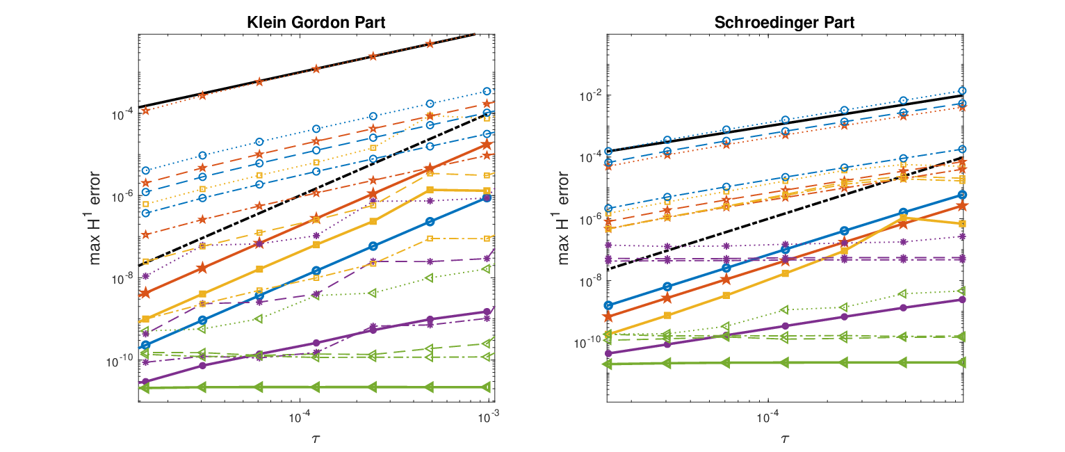
We dedicate this last section to the numerical verification of our results. We mainly concentrate on the convergence of the first order method in order to illustrate the explicit relation in our error estimates between gain in $c^{-2\alpha}$ , $0\leq\alpha\leq 1$ , for large $c$ , and consequent loss in derivative. In particular, we observe uniform accuracy and and improvement in convergence for more regular initial data and large $c$ , as depicted in Theorem 3.6. Then we briefly present the convergence results for the second order method, which verify second order convergence and uniform accuracy, as obtained in Theorem 4.10. We leave out the experiments for different regularity assumptions in this case for the sake of brevity. For the spatial discretisation we use a standard Fourier pseudospectral method, choosing $M=200$ as the highest Fourier mode. See [19] for more information on this technique as well as for some applications.

In Figure 1 we plot the global error of the first order scheme given by (15) and (19) measured in $H^{1}$ for different values of $c$ and initial data in Sobolev spaces varying in regularity, as well as the convergence of the second order scheme given by (35) and (48) measured in $H^{1}$ for different values of $c$ and smooth initial data.

Refer to caption — Figure 1: Convergence plot of the first and second order scheme given by (15), (19) and (35), (48). The blue, orange, yellow, purple and green lines correspond to the values of $c=1$ , $c=10$ , $c=100$ , $c=1000$ and $c=10000$ respectively. The black thick lines are reference lines of slope one and two. The ticker solid lines correspond to the second order scheme with smooth initial data. The thinner dotted, dashed and mixed lines correspond to the first order scheme with $H^{2}$ , $H^{3}$ and $H^{4}$ initial data respectively.

Acknowledgements

The author has received funding from the European Research Council (ERC) under the European Union’s Horizon 2020 research and innovation programme (grant agreement No. 850941).

References

[1] W. Bao, X. Dong, Analysis and comparison of numerical methods for the Klein-Gordon equation in thenonrelativistic limit regime, Numer. Math., 120 (2012), pp. 189–229
[2] W. Bao, L. Yang, Efficient and accurate numerical methods for the Klein-Gordon-Schrödinger equations, J. Comput, Phys., 225 (2007), pp. 1863-1893
[3] W. Bao, X. Zhao, A asymptotic consistent (UA) multiscale time integrator Fourier pseudospectralmethod for the Klein-Gordon-Schrödinger equations in the nonrelativistic limit regime, Numer. Math.,135 (2017), pp. 833–873
[4] S. Baumstark, G. Kokkala, K. Schratz, A Asymptotic consistent exponential-type integrators for Klein-Gordon-Schrödinger systems from relativistic to non-relativistic regimes, ETNA 48, pp. 63-80 (2018)
[5] M. Cabrera Calvo, K. Schratz, Uniformly accurate low regularity integrators for the Klein–Gordon equation from the classical to non-relativistic limit regime, https://arxiv.org/abs/2104.11672
[6] D. Cohen, E. Hairer, C. Lubich, Long-time analysis of nonlinearly perturbed wave equations viamodulated Fourier expansions, Arch. Ration. Mech. Anal., 187 (2008), pp. 341–368
[7] E. Faou, Geometric Numerical Integration and Schrödinger Equations, European Mathematical Society,Zürich, 2012
[8] E. Faou, K. Schratz, Asymptotic preserving schemes for the Klein-Gordon equation in the non-relativistic limit regime, Numer. Math., 126 (2014), pp. 441–469
[9] I. Fukuda, M. Tsutsumi, On the Yukawa-coupled Klein-Gordon-Schrödinger equations in three spacedimensions, Proc. Japan Acad., 51 (1975), pp. 402–405
[10] I. Fukuda, M. Tsutsumi, On coupled Klein-Gordon-Schrödinger equations. II, J. Math. Anal. Appl., 66 (1978), pp. 358–378
[11] I. Fukuda, M. Tsutsumi, On coupled Klein-Gordon-Schrödinger equations. III. Higher order interaction, decay and blow-up, Math. Japon., 24 (1979/80), pp. 307–321
[12] E. Hairer, C. Lubich, Modulated Fourier expansions for continuous and discrete oscillatory systems in Foundations of Computational Mathematics, Budapest 2011, F. Cucker, T. Krick, A. Pinkus, andA. Szanto, eds., vol. 403 of London Math. Soc. Lecture Note Ser., Cambridge Univ. Press, Cambridge,2013, pp. 113–128
[13] E. Hairer, C. Lubich, G. Wanner, Geometric Numerical Integration. Structure-Preserving Algorithms for Ordinary Differential Equations. Second Edition. Springer 2006
[14] E. Hairer, S. P. Nørsett, G. Wanner, Solving Ordinary Differential Equations I. Nonstiff Problems. Springer, Berlin, 1993
[15] M. Hochbruck, C. Lubich, A Gautschi-type method for oscillatory second-order differential equations, Numer. Math. 83:403–426 (1999)
[16] M. Hochbruck, A. Ostermann, Exponential integrators, Math. Ann., 324 (2002), pp. 359–389
[17] N. Masmoudi, K. Nakanishi, From nonlinear Klein-Gordon equation to a system of coupled nonlinear Schrödinger equations, Acta Numer., 19 (2010), pp. 209–286
[18] F. Rousset, K. Schratz, A general framework of low regularity integrators, to appear in SIAM J. Numer. Anal., http://arxiv.org/abs/2010.01640
[19] J. Shen, T. Tang, L.-L. Wang, Spectral methods: algorithms, analysis and applications, volume 41. Springer Science & Business Media (2011)

$\displaystyle\\|\mathcal{R}_{1}\\|_{r}$	$\displaystyle\leq\bigg\\|ic\langle\nabla\rangle_{c}^{-1}e^{i\tau c\langle\nabla\rangle_{c}}\int_{0}^{\tau}e^{-isc\langle\nabla\rangle_{c}}\big(e^{-i\frac{1}{2}s\Delta}\overline{\psi(t_{n})}\big)\mathcal{I}_{\psi}(s)\,ds\bigg\\|_{r}$	(9)
	$\displaystyle+\bigg\\|ic\langle\nabla\rangle_{c}^{-1}e^{i\tau c\langle\nabla\rangle_{c}}\int_{0}^{\tau}e^{-isc\langle\nabla\rangle_{c}}\big(e^{i\frac{1}{2}s\Delta}{\psi(t_{n})}\big)\mathcal{I}_{\psi}(s)\,ds\bigg\\|_{r}$
	$\displaystyle+\bigg\\|ic\langle\nabla\rangle_{c}^{-1}e^{i\tau c\langle\nabla\rangle_{c}}\int_{0}^{\tau}e^{-isc\langle\nabla\rangle_{c}}\big\|\mathcal{I}_{\psi}(s)\big\|^{2}ds\bigg\\|_{r}$
	$\displaystyle\leq\tau^{2}K\big(\sup_{0\leq\xi\leq\tau}\\|\psi(t_{n}+\xi)\\|_{r}\big),$

	$\displaystyle\\|\mathcal{R}^{\prime}_{3}\\|_{r}$	$\displaystyle\leq\bigg\\|ic\langle\nabla\rangle_{c}^{-1}\int_{0}^{\tau}e^{-isc\langle\nabla\rangle_{c}}\|\mathcal{I}_{\psi}(s)\|^{2}ds\bigg\\|_{r}$		(22)
		$\displaystyle\leq\tau^{3}K\big(\sup_{0\leq\xi\leq\tau}\\|u(t_{n}+\xi)\\|_{r},\sup_{0\leq\xi\leq\tau}\\|\psi(t_{n}+\xi)\\|_{r}\big),$		(22)

$\displaystyle\\|\mathcal{R}^{\prime\prime}_{3}\\|_{r}$	$\displaystyle\leq\bigg\\|e^{i\frac{1}{2}s\Delta}\int_{0}^{s}e^{-i\frac{1}{2}\sigma\Delta}\mathcal{I}_{\psi}(\sigma)\big(e^{i\sigma c\langle\nabla\rangle_{c}}u(t_{n})+e^{-i\sigma c\langle\nabla\rangle_{c}}\overline{u(t_{n})}\big)d\sigma\bigg\\|_{r}$	(23)
	$\displaystyle+\bigg\\|e^{i\frac{1}{2}s\Delta}\int_{0}^{s}e^{-i\frac{1}{2}\sigma\Delta}\big(e^{i\frac{1}{2}\sigma\Delta}\psi(t_{n})\big)\big(\mathcal{I}_{u}(\sigma)+\overline{\mathcal{I}_{u}(\sigma)}\big)d\sigma\bigg\\|_{r}$
	$\displaystyle+\bigg\\|e^{i\frac{1}{2}s\Delta}\int_{0}^{s}e^{-i\frac{1}{2}\sigma\Delta}\mathcal{I}_{\psi}(\sigma)\big(\mathcal{I}_{u}(\sigma)+\overline{\mathcal{I}_{u}(\sigma)}\big)d\sigma\bigg\\|_{r}$
	$\displaystyle\leq s^{2}K\big(\sup_{0\leq\xi\leq\tau}\\|u(t_{n}+\xi)\\|_{r},\sup_{0\leq\xi\leq\tau}\\|\psi(t_{n}+\xi)\\|_{r}\big),$

	$\displaystyle\\|u(t_{n})-u^{n}\\|_{r}$	$\displaystyle\leq\tau^{2}K\big(\sup_{t_{n}\leq t\leq t_{n+1}}\\|u(t)\\|_{r+2},\sup_{t_{n}\leq t\leq t_{n+1}}\\|\psi(t)\\|_{r+2}\big)$
		$\displaystyle+\tau^{2}c^{-2\alpha}K\big(\sup_{t_{n}\leq t\leq t_{n+1}}\\|u(t)\\|_{r+2\alpha+2},\sup_{t_{n}\leq t\leq t_{n+1}}\\|\psi(t)\\|_{r+2\alpha+2}\big)$
		$\displaystyle+\tau^{2}c^{-4\alpha}K\big(\sup_{t_{n}\leq t\leq t_{n+1}}\\|\psi(t)\\|_{r+4\alpha+5}\big),$