Density reconstruction from schlieren images through Bayesian nonparametric models
Abstract
This study proposes a radically alternate approach for extracting quantitative information from schlieren images. The method uses a scaled, derivative enhanced Gaussian process model to obtain true density estimates from two corresponding schlieren images with the knife-edge at horizontal and vertical orientations. We illustrate our approach on schlieren images taken from a wind tunnel sting model, a supersonic aircraft in flight, and a high-order numerical shock tube simulation.
Keywords Gaussian process Bayesian inference Schlieren
1 Introduction
Since its inception in the late-17th century by Robert Hooke, schlieren has been used in the sciences, engineering and even the arts. The types of flows captured have been diverse spanning the shock waves formed around a supersonic aircraft; the mixing of turbulent jets; plume formation over a candle, and even the dissolution of particles in a solution. Scientifically, these images have shaped our understanding of fluid mechanics. More broadly, they have, and continue to, inspire and captivate a collective curiosity about the natural world.
A schlieren is governed by refractive behaviour of light when passing through a medium. For instance, when encountering a homogeneous medium, light rays will pass through uniformly, but if the light rays pass through regions of inhomogeneity, they will refract in proportion to the gradient of the refractive index of the inhomogeneities (Rienitz, 1975; Settles, 2001).
Flow phenomena such as shock waves, jets and plumes can cause variations in the density of air, leading to refractions that can be captured by a focused, one-to-one optical image. Consider the simplest of schlieren setups: a point light source-based experiment that requires two convex lenses, a knife-edge, and a camera, as shown in Figure 1. With the point light-source being the initial illuminator, the light is collimated by the first lens, and then refocused to a single point by the second lens where a knife-edge is positioned. The light rays then travel past the knife-edge to cast an inverted image upon an appropriately placed screen. The area between the two lenses represents the test section where the object of interest should be placed. The knife-edge, which can be a standard razor, misses the upward deflected array, but blocks the downward deflected array. As a result the upward deflected array appears on the screen as a bright spot, while the downward deflected array leaves a dark spot. The knife-edge effectively transforms an invisible phase difference between the light rays to a visible amplitude change, which is recorded on the screen as a change in the refractive index11 1 The refractive index is given by the speed of light through a given medium divided by the speed of light in vacuum. Depending on the orientation of the knife-edge, either the horizontal or the vertical gradient of the refractive index can be visible. Although this description is of the most primitive of schlieren setups, it does capture the governing physics. In this case, a point-light source is assumed, while in general, an extended light source would be used which would require a focusing lens to be positioned between the knife-edge and the screen (Settles, 2001).
The utility of a schlieren image lies in the fact that the refractive index is dependent on the density of the medium it passes through. Knowledge of this relationship permits one to obtain quantitative data from such images. To make this lucid, let be the spatially varying density of a fluid surrounding an object of interest; it is expressed as a scalar-field with a horizontal coordinate and a vertical coordinate . It has a linear relationship with the refractive index , given by
| (1) |
where is the Gladstone-Dale coefficient. A schlieren image represents the refractive index gradient field , where the gradient direction is based on the orientation of the knife edge: placement in the vertical direction yields , whilst placement along the horizontal direction renders (Hargather and Settles, 2012).
There are two points to note regarding the overall quality of a schlieren image. First, the diffraction of light from the object of interest can degrade the quality of the schlieren image. This may be exacerbated around the edges of the test object where halos are found to appear. However, these do not introduce a significant impediment when used for quantitative analysis as they do not obscure the flow detail (Kumar et al., 2008). Second, is the prominence of dark regions in the schlieren image where it should be bright—this is suggestive of a region with high density gradients, where the light rays are highly refracted and blocked by some component in the schlieren set-up such as the knife-edge/lens mount (Settles, 2001). This may limit the accuracy of quantitative (and indeed qualitative) information that may be extracted from the region and its vicinity.
As mentioned previously, schlieren experiments have been conducted for a wide range of flows since its inception, however, it should be noted that it can be difficult to find an image pair corresponding to a vertical and horizontal knife-edge result in literature, with the vast majority of published results focusing on only one of the two knife-edge orientations. Additionally, the quality of published images can vary due to a wide range of reasons. One commonly seen issue with such images is over-ranging of the schlieren system, where too much knife-edge cutoff is used which leads to large areas showing up as extreme bright and dark regions, concealing the underlying flow features (Settles, 2001). Another commonly found issue is with older publications, where papers have been digitised, but with the pixel values of source images being subject to thresholding - resulting in much of the flow details being lost. While there have been a large number of schlieren images generated in literature, it is important to note their quality can vary widely due to the aforementioned reasons.
Consider some of the earlier work conducted at the National Aeronautics and Space Administration (NASA) (or more specifically its predecessor the National Advisory Committee for Aeronautics (NACA)) where a significant number of schlieren results have been digitised, but without the same quality as a digitally captured image due to the digitisation process. With either significant noise being introduced, or the image pixel values being curtailed resulting in missing flow features and details. Some examples of such images can be found in the following references (Daley et al., 1948; Lindsey et al., 1952; Erdmann, 1953; W. G. et al., 1965). It is important to note that such images would generate poor results with the proposed method.

1.1 Supersonic flow behaviour
When an object is immersed in transonic or supersonic flow, thin regions of discontinuity can form across which flow properties change rapidly. Across these shock waves, static flow properties such as pressure, density, temperature and entropy increase, while the stagnation pressure, Mach number and velocity decrease (Anderson, 2011). Oblique shock waves form across concave corners, where the shocks generally form at an oblique angle (less than ). In regions of convex corners, the opposite effect occurs, resulting in expansion fans, across which the static pressure, density, and temperature decrease, while the Mach number increases. This is shown in Figure 2, where the flow follows the path from to across an expansion fan with an expansion angle .


As the flow must be tangential to the wall at all times, the streamlines will follow the direction of the wall. When considering a two-dimensional supersonic flow over a wedge, a sharp change in the direction of the streamline occurs across the shock. However, when considering three-dimensional supersonic flow over a cone, there is a third dimension for the air to pass through, leading to a “three-dimensional relieving effect” that renders a smoother transition to the new wall angle (see Figure 3). This has the added effect of creating a weaker shock wave than a wedge shock with the same wall angle () and inflow properties. Hence, under the same conditions. Apart from the weaker shock and the less adverse streamlines, the flow behaviour is similar between the wedge and the cone.
Assuming a steady state shock in a predominantly inviscid flow (except near the shock) under adiabatic conditions, the downstream Mach number and density across an oblique shock wave for a wedge, is given by (see page 623 in Anderson, 2011)
| (2) |
where, is the wave angle, is the deflection angle, is the specific heat ratio, and are the downstream Mach and density. These expressions, in tandem with other isentropic flow relations, may be used to estimate density from other observed thermodynamic quantities.
1.2 Quantitative analysis
Although predominantly used for qualitative assessments, there is a considerable body of literature devoted to the singular task of extracting quantitative information from schlieren images (Hargather and Settles, 2012; Wildeman, 2018; Hay et al., 2019; Tobin and Hargather, 2016; Venkatakrishnan, 2005; Dalziel et al., 2000). While a typical qualitative analysis may study the visible shock angles and refraction patterns, a quantitative analysis focuses on extracting primitive flow field variables—e.g., density, temperature or velocity from schlieren images. The overarching framework relies on being able to relate the pixel values across the image to a known refraction angle (Settles, 2001; Settles and Hargather, 2017). We remark that our definition of quantitative in this study refers strictly to the extraction of the density scalar field from schlieren images.
1.2.1 Image pre-processing
Depending on the schlieren set-up, images may require some level of pre-processing to account for poor contrast, brightness, and sharpness (to name a few factors) before use in quantitative analysis. The pixel-values of a schlieren image do not necessarily always encompass the entire 256 levels of greyscale possible; instead the brightest pixel may be a fraction of this. By setting the value of the brightest pixel to the highest greyscale level of 256, and proportionally increasing the value of the rest of the pixels, we can form a new image with a higher contrast. This is known as contrast stretching. The brightness of an image can be increased by simply increasing all the pixel values by a constant, with a maximum limit set to 256. The sharpness of the image can be improved using sharpening techniques such as unsharp masking. This method uses a mask created by the difference between the source image and a blurred version of the image to detect edges. The contrast of the edges covered by the mask are increased to create a sharper image (See Section 3.2.4 in Settles, 2001 for pre-processing techniques for schlieren images).
1.2.2 Calibrated Schlieren
The most straightforward approach to extract quantitative data from a schlieren image is to place a calibrated object with a known refractive index in the test area. This would facilitate the generation of a map between the pixel intensity and the refractive index gradient. Typically, a lens is used, with each radial position across the lens having a different refraction angle (or refractive gradient) to focus the collimated light. The focal length of the calibration lens determines the resolution of the refractive index variations, with finer resolutions being obtainable with longer lenses. Imaging using this setup yields the calibration required between the pixel intensity and the true refractive index gradient. The refractive index gradient field is integrated to obtain the refractive index which is converted to a density field using the Gladstone-Dale relationship from (1), with a known density value used to solve for the constant of integration (typically the known free-stream density). This assumes the fluid under consideration is not a mixture of gases, and hence has a constant value of . To be able to quantify for a mixture of gases, an estimate for the Gladstone-Dale constant, would be required (Settles, 2001; Settles and Hargather, 2017).
1.2.3 Rainbow Schlieren
Rainbow schlieren (discovered by Schardin, 1942; Vandiver, 1974, but termed by Howes (Howes, 1983; Howes, 1984)) substitutes a knife-edge with a radial rainbow cut-off filter with a continuous spectrum to generate an image with hue variations. The light passing through the colour cut-off filter will take the hue corresponding to its path along the filter. As the rainbow filter is continuous—i.e., without any sharp edges or discontinuities—errors due to diffraction are effectively non-existent. The replacement of the filter leads to refractive index gradients being displayed as variations in colour rather than irradiance (Hargather and Settles, 2012). Use of the colour filter by itself does not provide vastly more information over the standard greyscale schlieren image. However, its advantage lies in the ability to use different colour filters to colour-code targeted refraction directions/magnitudes. For example, the use of a bulls-eye pattern would highlight the refraction magnitudes that occur in the radial direction. Obtaining quantitative data from this setup would follow the described calibration approach from above, but instead of the pixel intensity of a greyscale schlieren image, the hue from a colour schlieren image would be mapped to the known refraction angle (Settles, 2001; Settles and Hargather, 2017).
1.2.4 Background Oriented Schlieren (BOS)
The premise of BOS is to measure the level of distortion in a background pattern with and without the refractive disturbances. This method requires little set-up and equipment as only a high resolution camera is required, and possibly a background pattern depending on whether the natural background behind the object of interest has sufficient variation for image processing to pick up patterns and image distortion artefacts (Hargather and Settles, 2012; Heineck et al., 2016; Heineck et al., 2021). Venkatakrishnan, 2005 demonstrated the construction of a density field using BOS for a cone-cylinder flow at Mach 2.0. Additionally, work conducted by NASA has led to the use of natural backgrounds to capture schlieren images of different aircraft by using the sun/sky as the background (Heineck et al., 2019; Hill and Haering, 2017a; Hill and Haering, 2017b).
To estimate the density field using BOS, a reference image of a structured background pattern without density gradients is taken, along with another image with the refractive disturbances active. The displacements along and in the background pattern are computed between these two images using cross-correlation, and used to estimate a source term , which is the sum of the derivative of the density gradients. The individual density derivatives can then be obtained by substituting the empirical values of in Poisson’s equation
| (3) |
with appropriate boundary conditions (see 6 in Venkatakrishnan and Meier, 2004). Note that this provides a projection of the 3D density field in the camera direction, i.e. it is the integrated density distribution across the line of sight. By using standard tomographic reconstruction techniques such as filtered back-projection, the density field across a plane of interest can be obtained (Venkatakrishnan, 2005).
More quantitative methods such as absolute and standard photometry methods are described in detail in Settles, 2001, Chapter 10. We omit an exposition of these methods here for brevity. It is important to note that all prior quantitative methods are limited, i.e., they require either a special apparatus with a reference calibration within the image, or multiple images of the same object with control over a refractive distortion. This makes it particularly difficult to re-create density fields of past schlieren images—especially those that were taken with only a qualitative analysis in mind. Additionally, none of these methods offer a comprehensive pathway to account for the uncertainties in the density (or other thermodynamic quantities).
2 Pixels to Density via Machine Learning
Our approach to schlieren imaging in this paper takes a decidedly different path from the quantitative efforts referenced above. We leverage ideas from machine learning, namely Gaussian process regression (Rasmussen and Williams, 2006), to facilitate the spatial estimation of density.
2.1 From schlieren to density
Our goal in this subsection is to derive a formulation that maps one, or two, schlieren images—of the same observation taken with two different knife-edge orientations—to a spatial density estimate. A natural starting point is (1), that relates the refractive index with density. Taking partial derivatives with respect to and yields
| (4) | ||||
| (5) |
The left-hand side of (4) and (5) is the partial derivative of the refractive index. Pixel intensities in a given schlieren image are linearly related to their corresponding refractive index partial derivatives. In other words, a schlieren image taken with a vertical knife-edge is a function of , and a schlieren image taken with a horizontal knife-edge is a function of . The simplest way to characterise this linear relationship is
| (6) | ||||
| (7) |
where and are the pixel intensities in a schlieren image. Note that all the terms on the right-hand side of (6) and (7) barring and are constants. This includes , which will vary depending on the brightness, contrast, and other histogram-based image processing choices. To clarify, there may be cases where both and will be 255, leading to both and to be zero.
2.2 Schlieren-based Gaussian process model
We now build a Gaussian process (Rasmussen and Williams, 2006) model to statistically infer the density given one or two schlieren images. To ease our exposition, we enumerate the model training and the model prediction data below, where the abbreviation “loc.” denotes locations and “out.” denotes outputs.
Quantity
Training loc.
Training out.
Training noise
Prediction loc.
Prediction out.
Schlieren
(vertical)
Schlieren
(horizontal)
Density
To crystallise the precise form of the model inputs, consider the schematic shown in Figure 4. Each row represents a possible combination of model inputs. In the top row, the grid of points represent training locations taken from both (a) horizontal (b) and vertical schlieren images, along with (c) three density spatial locations. Sub-figures (d-e) represent spatial samples associated with only the (d) horizontal schlieren image and (e) two density input locations. Lastly sub-figures (f-g) show the (f) vertical schlieren image and (g) two density input locations. As we will see later, the distinction between a model input with one or two schlieren images will have effect the output spatial density estimates. We remark here that while the input spatial locations for the schlieren images in Figure 4 are shown as a uniform grid, in practice one can resort to non-uniform sampling with the aim of delivering a better resolution of certain spatial characteristics.

In table 1, each row has an associated training noise that attributes an uncertainty to the pixel and density values. This uncertainty is assumed to have a zero-mean Gaussian distribution. Throughout this paper, we further assume that these covariance matrices have the form , , and , where is the identity matrix and standard deviations and will be assigned.
It is important to note that the quality of the schlieren images does have a direct impact on the reliability of the result generated using this method. Source images where there are regions with thresholded values, clipping or large amounts of noise in general (e.g. due to digitisation) are not good candidates for this method since it can produce non-physical or poor results.
2.2.1 Model prior
Standard Bayesian formalism requires the definition of a model likelihood and a model prior. The model likelihood is set by the data and the noise, while the model prior in a Gaussian process context is set by the mean and covariance function. To this end, we assume that the spatial density field—which we seek to infer—bounded by the image domain is a Gaussian random field with some mean and covariance function. Were we to select a few spatial samples from this field, they would represent a Gaussian distribution specified entirely by the mean and covariance (Rasmussen and Williams, 2006).
Note from (10), schlieren images are described as linear operators acting over the density field. By assuming that the density field is a Gaussian random field, and that the schlieren images are effectively linear operators acting over this random field, a gradient-based Gaussian process framework for extracting the density can be derived. The joint Gaussian density across the training data (see first three columns of Table 1) is written as
| (11) |
where denotes a vector of ones of length specified by its subscript. Matrices given by the symbol are used to denote a kernel function evaluated at the spatial locations provided as the arguments. Element-wise entries of the relevant blocks of the covariance matrix in (11) are given by
| (12) | ||||
It is important to note that in (11) must be symmetric positive definite for the chosen kernel function . The predictive mean for the two schlieren images and the density may then be computed as
| (13) |
with representing the stacked training data outputs as per (11). The predictive covariance is written as
| (14) |
where the individual covariance matrix blocks follow the same notation in (12) trading the training location subscripts with the prediction locations as per Table 1.
A few comments on the above are in order. First, our model is distinct from the standard gradient enhanced Gaussian process model (Särkkä, 2011) (also known as Gradient-Enhanced Kriging (Lockwood and Anitescu, 2012; Ulaganathan et al., 2015; Ulaganathan et al., 2016; Wu et al., 2017; Chen et al., 2019; Bouhlel and Martins, 2019)) as we are not strictly observing gradients, but some linear function of the gradients following (10). Second, while there is considerable flexibility in defining the kernel function, it must be twice differentiable. One obvious choice is the squared exponential function
| (15) |
that is parameterised by a signal noise variance and a length scales and . Expressions for
| (16) |
are trivially derived and used in (12). Other valid kernel choices include a Fourier series kernel (Seshadri et al., 2022), a Matérn kernel (Rasmussen and Williams, 2006), among others.
A subset of the joint distribution defined in equation (11) can be used if an image is available for only one gradient direction with the caveat that the posterior mean will not fully represent the density field unless the flow is highly directional and the gradient in the other direction is negligible.
2.2.2 Prior definition
Unknown parameters associated with both the kernel function and the overarching model can be grouped into a vector . By incorporating knowledge of the potential range or physical nature of the model, it is possible to prescribe a set of prior probability distributions . If knowledge regarding the observed data is unknown, this can be captured by a prior distribution with a large variance. In this study, prior distributions are defined for with reduced model complexity to allow for generalisation of the model to multiple cases. To ensure a positive semi-definite covariance matrix, the hyperparameters defined here must be positive. Additionally, to ensure that the length scales and kernel noise terms are not wildly different at the gradient- and functional levels, we introduce a re-parameterisation of the form
| (17) |
where, , , , and are assigned half-normal prior distributions. With this new prior definition, we set . When observation data for only schlieren image is available, the hyperparameters simplify to the original .
2.2.3 Hyperparameter optimisation
These free hyperparameters () require tuning to find the optimal values to give the expected posterior mean. This can be via a straightforward grid or random search but with the downside of being intractable when working with a larger number of hyperparameters (Claesen and Moor, 2015). There are instead automated methods that approach this search from a more analytical perspective.
A well-worn approach is to maximise the logarithm of the marginal likelihood, conditioned on the hyperparameters (Rasmussen and Williams, 2006). The values found from such a method are such that they maximise the likelihood that the user-specified model produces the data that is observed.
| (18) |
where the mean and covariance terms are evaluated at the observed data only. A more developed approach is the Maximum a Posteriori (MAP) estimation method which in addition to the log-likelihood () takes advantage of knowledge in the prior distribution with the term. The prior distribution creates a bias of the probability mass density towards regions that are preferred a priori (Goodfellow et al., 2016), which can be advantageous when trusted prior knowledge of the observed data is available.
| (19) |
Both the marginal likelihood and MAP make predictions based on a point estimate of which can be advantageous from a performance standpoint, but have the side-effect of focusing on a local maxima and not widely exploring the probability space. Ideally, a fully Bayesian approach would be used where instead of a point estimate, predictions would be made with a full distribution over , where, for each observed sample, either a positive probability would contribute for the next sample and any uncertainty would be accounted for in any predictions made (Goodfellow et al., 2016). However, it is intractable to attempt to make predictions using a full posterior distribution over .
One approach to achieve an estimated result is by approximating the posterior distribution by random sampling. A popular method is Markov chain Monte Carlo (MCMC). MCMC can also be used to generate an estimate of the posterior distribution where it cannot be calculated analytically. MCMC performs approximate integration by drawing samples from the posterior distribution and performing sample averages. The Markov chain refers to the drawing of samples, where, the next sample drawn is dependent on the previous, and Monte Carlo is the technique used for random sampling of the posterior distribution for integration (Goodfellow et al., 2016). By running multiple chains concurrently with varying starting points, it is possible to capture multiple states of equilibrium unlike the point estimate approaches.
2.2.4 Computational Considerations
Computing the direct inverse of covariance matrices in equations 13, and 14 can be slow and numerically unstable. If one were to use a standard approaches, such as an LU decomposition to find the inverse, the cost would be in the order for an n-dimensional matrix (Gibbs et al., 1997). By considering the symmetric and positive-definite nature of the covariance matrix, the Cholesky decomposition can instead be used which exploits the symmetry to cost half that of the LU (Trefethen and Bau, 1997) factorisation. This cost can be intractable for larger datasets, especially when applying Bayesian approach to optimise for kernel hyperparameters (), where is evaluated repeatedly with varying . There are many approaches in literature that aim to solve this issue, either by creating low-rank approximations of at the cost of accuracy, by exploiting the sampling structure to break down the inversion to more efficient matrix vector products, or through iterative approximations such as the conjugate gradient method (Gilboa et al., 2015; Shen et al., 2005; Gibbs, 1998; Skilling, 1993).
One approach to reduce computational cost is through the use sparse GPs that approximate the posterior with pseudo-training points (known as inducing points, ) that are located within the domain. If the original number of training inputs is , with < , the original cost of direct covariance matrix inversion is reduced down to . Two such commonly used sparse approximation methods are FITC (fully independent training conditional) (Snelson and Ghahramani, 2005; Quiñonero-Candela and Rasmussen, 2005), and VFE (variational free energy) (Titsias, 2009).
Work by Saatçi, 2011 demonstrates the use of a grid structure for training points which results in a covariance matrix where Kronecker products can be used to efficiently complete Gaussian regression in . Due to the non-collocated nature of the approach in this study (between the gradient and function sampling), the gradient inputs may be sampled from an image in a grid format, however the addition of the function observations disrupts the required format to take advantage of Kronecker products directly, without any masking of regions. Since this paper is purely focused on the methodology of obtaining quantitative data from schlieren images, only some of these approaches have been considered to make the method tractable.
3 Results

This paper offers a radically different way to think about schlieren, whilst staying true to its fundamental physics, building upon our preliminary work towards quantitative schlieren using machine learning (Ubald et al., 2021). An overview of the present workflow is illustrated in Figure 5. In the results that follow, we report the mean and standard deviation, i.e., output by our model. As these moments are for the density field, both have units of .
It should be noted that unless otherwise stated, that a down-sampled version of the image is used as input in each case due to the computational cost. Additionally, Matérn 3/2 and 5/2 kernel functions were also used to compare against the squared exponential kernel function defined in equation 12 for the first case, all kernel functions obtained comparable predictions of density. However, the Matérn kernels were more onerous to optimise for compared to the squared exponential, hence, for all studies in this paper, the squared exponential kernel function is used.
3.1 Wind tunnel sting model
Consider the asymmetrical sting model in supersonic flow ( 2.0) published by Ota et al., 2011. The reconstructed density published in that paper, using BOS, is assumed to be representative of the true density, and thus serves as our benchmark for comparison. Figure 6 captures the experimental results with the vertical knife-edge schlieren image in (a); horizontal knife-edge schlieren image in (b), and the BOS yielded density reconstruction in (c). Note that for subfigures (a) and (b) the colours denote greyscale pixel values between , whilst the colours in (c) represent the density in units of . Another point to note is that only the upper half of the schlieren images are used for this reconstruction, as the shock captured across the lower half sees excessive clipping.


The reconstructed density is shown in Figure 7 with the mean in (a) and the standard deviation in (b). The mean follows the expected trend of a uniform density upstream of the shock followed by a rapid increase in density across the shock, before decreasing across the expansion fan. Due to clipping of the input schlieren images, the gradients in region downstream of the expansion fan are not captured (the gradients are close to zero), hence this is represented as the mean of the observed densities instead. We remark that the BOS density in subplot Figure 6(c) does not follow the expected behaviour of oblique shocks in theory, where, the density upstream of the shock must be uniform with a sharp increase in density across the shock. This may be caused by optical distortion incurred when performing BOS. Additionally, the shock itself should be captured as a very thin band, which is what is captured in our reconstruction, along with the shear layer downstream.

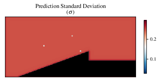
It is possible to obtain some results using partial gradient observation, i.e., using either vertical or horizontal knife-edge schlieren as input. An example of the density prediction using the same workflow as above, but using only vertical knife-edge as input is shown in Figure 8(a). A semblance of the shock is formed with this approach, but is not fully formed since the density gradient is directional, but the shear layer downstream is captured. The lack of additional gradient input is captured by the higher standard deviation in the prediction (Figure 8(b)).
3.2 Supersonic aircraft in flight
Next, we study schlieren images taken by NASA of a T-38 training jet at a Mach number of 1.05. The horizontal and vertical knife-edge schlieren images captured by Heineck et al., 2016; Heineck et al., 2021 are shown in Figure 9(a) and (b) respectively. Additionally, based on estimates of the ambient conditions of the flight and estimates of shock and wedge angles, we can estimate the density at three points as shown in Figure 9(c). The two freestream points are assigned the same value of density, whilst the density at the third (remaining) point is estimated via the shock relations in section 1.1.

As true density fields are not available for this case, and at least one known density is required from a non-freestream region for this method, the density after the first oblique shock wave is estimated. Two quantities are used to calculate the density: (i) the known experimental altitude of 30,000 ft and thus the freestream density; (ii) the shock relations in Equation 2, accounting for uncertainties in the Mach number and angles. However, note that this is a simplification, as the wedge angle calculation does not account for the three-dimensional relief effect. The flow conditions at this altitude and the estimated uncertainties are listed in the appendix in Table 7. This density data, along with horizontal and vertical knife-edge schlieren images are sub-sampled (to reduce the computational overhead), and fed into the machine learning workflow. For the inputs to the GP, the aircraft region is masked out, as it is the geometry and is not part of the flow.
The predicted density and standard deviation are shown in Figure 10, with each shock clearly visible in the prediction. In addition to this, by focusing in on the downstream wake region (highlighted blue section in Figure 9(c)), the wake prediction can be seen in more detail, with the wake trail clearly being captured by the prediction.
3.3 Shock tube CFD
In this section, we consider a canonical Sod shock tube (Sod, 1978) test case. The CFD simulation result provided by Dzanic and Witherden, 2022 is used, with the full primitive flow variables available for comparison. Figure 12 shows a set of results from one timestep that are used as inputs to the GP. To simulate a schlieren image, the density gradient is calculated, and normalised to standard pixel value range of between 0 and 255. Figure 12 shows the vertical knife-edge schlieren result in (a); horizontal knife-edge schlieren image in (b), and the true density obtained by CFD (c).
4 Conclusions and Future Work
We have demonstrated the development of a method to obtain quantitative density data from pre-existing Schlieren images through the use of Gaussian processes. The central novelty with this method lies in the fact that it does not require any pre-calibration or special set-up as required by existing methods discussed in Section 1.2, and is widely applicable—even if only one knife-edge orientation is available. Our workflow is not intended to upend or subvert the modern practicalities of BOS, but rather complement it, by enabling scientists to be able to retrospectively reconstruct density fields from the plethora of schlieren images that exist in literature.
Future work will study the use of the above methodology for schlieren videos, which will incorporate a temporal kernel that relates successive frames of a video. Beyond this we plan to explore the use of deep Gaussian processes to facilitate more accurate flow feature representations.
Appendix A Appendix
In this section we present a validation of our approach along with supplemental particulars for the two examples provided above.
A.1 Method validation with synthetic Schlieren images
A simple analytical function is used to define a model density field and its corresponding density gradient. The density gradients are normalised to pixel values () to emulate a Schlieren image with an unknown range, and a random sampling of 200 are selected from this image for use as observation data (white circles in Figure 14), with three random density sampling locations also used (green circles in Figure 14). The density and its partial derivative w.r.t and for this case are given as
| (20) |

| Parameter | Distribution | Moments |
|---|---|---|
| half-normal | ||
| half-normal | ||
| half-normal | ||
| deterministic | 1E-3 | |
| deterministic | 0.1 |
The prior definitions for this case are listed in Table 2, with Figure 15 showing a comparison of the true density (a) against the posterior predicted mean density (d), and the corresponding prediction of the gradients (e-f), and the posterior standard deviation shown in (g) exhibiting a generally uniform and small standard deviation demonstrates a high level of model confidence.


If the flow is highly directional, and the gradients in one direction dominate the flow, such is the case in this analytical function, where the gradients in are dominant. The joint distribution can be simplified to accept gradient input from only one direction, with simpler prior definitions as listed in Table 3. A comparison between the true and partially reconstructed density field shown in Figure 16 shows good agreement. Since the density gradient is highly directional, this method is still, able to capture the correct trends and provide an indicative result.
| Parameter | Distribution | Moments |
|---|---|---|
| half-normal | ||
| half-normal | ||
| half-normal | ||
| deterministic | 1E-3 | |
| deterministic | 0.1 |
A.2 Priors for the wind tunnel sting model
Priors for the wind tunnel sting model Gaussian process are given in Tables 4 and 5 for results with both schlieren images, and with only the vertical knife-edge image as inputs respectively. The lengthscales () for this case are defined based on the spacing between the training locations.
| Parameter | Distribution | Moments |
|---|---|---|
| deterministic | 0.67 | |
| deterministic | 0.675 | |
| half-normal | ||
| half-normal | ||
| deterministic | 1E-4 | |
| deterministic | 0.1 |
| Parameter | Distribution | Moments |
|---|---|---|
| deterministic | 0.5 | |
| deterministic | 0.2 | |
| half-normal | ||
| half-normal | ||
| deterministic | 1E-2 | |
| deterministic | 0.1 |
A.3 Priors for the supersonic aircraft in flight
Priors for the wind tunnel sting model Gaussian process are given in Table 6; flow properties used to estimate the density are provided in Table 7.
| Parameter | Distribution | Moments |
|---|---|---|
| half-normal | ||
| half-normal | ||
| half-normal | ||
| half-normal | 1.0 | |
| half-normal | 0.3 |
| Flow property | Value |
|---|---|
| 0.459 0.005 | |
| 0.5 0.06 | |
| 1.401 0.001 | |
| 1.05 0.05 | |
| 77∘ 2∘ |
A.4 Priors for the shocktube CFD case
Priors for the supersonic CFD Gaussian process are given in Table 8.
| Parameter | Distribution | Moments |
|---|---|---|
| half-normal | ||
| half-normal | ||
| half-normal | ||
| deterministic | 2.5E-4 | |
| deterministic | 1.0 |
Acknowledgments
Special thanks to Masanori Ota from Chiba University for kindly providing schlieren images of the asymmetric sting model for use as a test case. Thanks also to Tarik Dzanic from Texas A&M University for providing the CFD results for the Sod shock tube test case. Please note that the Schlieren aircraft images in Figures 5 and 9 are sourced from a United States government work (Heineck et al., 2016; Heineck et al., 2021) and are therefore not subject to copyright protection.
Funding Statement
The authors were partly supported by the Lloyd’s Register Foundation-Alan Turing Institute Strategic Priorities Fund. The fund is delivered by UK Research and Innovation, with this award managed by EPSRC (EP/T001569/1). PS also wishes to acknowledge the funding and support of Rolls-Royce plc.
Competing Interests
The authors declare no competing interests exist.
Data Availability Statement
The data and all aspects of the code that support the findings of this study, including the figure generation are openly available in the ‘dce-schlieren-density-reconstruction’ repository at ‘github.com’ (https://github.com/bnubald/dce-schlieren-density-reconstruction).
Ethical Standards
The research meets all ethical guidelines, including adherence to the legal requirements of the study country.
Author Contributions
Conceptualization: B.N.U.; P.S. Data curation: B.N.U. Formal analysis: B.N.U.; P.S. Investigation: B.N.U.; P.S. Methodology: B.N.U.; P.S. Project administration: B.N.U.; P.S. Software: B.N.U.; P.S. Supervision: P.S.; A.D. Validation: B.N.U. Visualization: B.N.U. Writing - original draft: B.N.U. Writing - review & editing: B.N.U.; P.S.; A.D. All authors approved the final submitted draft.
References
- Anderson, (2011) Anderson, J. D. (2011). Fundamentals of aerodynamics. McGraw-Hill, 5th edition.
- Bouhlel and Martins, (2019) Bouhlel, M. A. and Martins, J. R. (2019). Gradient-enhanced kriging for high-dimensional problems. Engineering with Computers, 35:157–173.
- Chen et al., (2019) Chen, L., Qiu, H., Gao, L., Jiang, C., and Yang, Z. (2019). A screening-based gradient-enhanced kriging modeling method for high-dimensional problems. Applied Mathematical Modelling, 69:15–31.
- Claesen and Moor, (2015) Claesen, M. and Moor, B. D. (2015). Hyperparameter search in machine learning. In MIC 2015: The XI Metaheuristics International Conference, pages 14–1–14–5. MIC.
- Daley et al., (1948) Daley, B. N., Humphreys, M. D., Field, L., Washington, V., Ton, M., and Humphreys, D. (1948). Effects of compressibility on the flow past thick airfoil sections.
- Dalziel et al., (2000) Dalziel, S., Hughes, G. O., and Sutherland, B. R. (2000). Whole-field density measurements by ‘synthetic schlieren’. Experiments in fluids, 28(4):322–335.
- Dzanic and Witherden, (2022) Dzanic, T. and Witherden, F. D. (2022). Positivity-preserving entropy-based adaptive filtering for discontinuous spectral element methods.
- Erdmann, (1953) Erdmann, S. F. (1953). A New Simple Interferometer for Obtaining Quantitatively Evaluable Flow Patterns. Technical memorandum. National Advisory Commitee for Aeronautics.
- Gibbs et al., (1997) Gibbs, M., Gibbs, M., and MacKay, D. J. (1997). Efficient implementation of gaussian processes.
- Gibbs, (1998) Gibbs, M. N. (1998). Bayesian gaussian processes for regression and classification.
- Gilboa et al., (2015) Gilboa, E., Saatci, Y., and Cunningham, J. P. (2015). Scaling multidimensional inference for structured gaussian processes. IEEE Transactions on Pattern Analysis and Machine Intelligence, 37:424–436.
- Goodfellow et al., (2016) Goodfellow, I., Bengio, Y., and Courville, A. (2016). Deep learning. The Mit Press.
- Hargather and Settles, (2012) Hargather, M. J. and Settles, G. S. (2012). A comparison of three quantitative schlieren techniques. Optics and Lasers in Engineering, 50(1):8–17.
- Hay et al., (2019) Hay, T. A., Valdez, J., Tinney, C. E., Hamilton, M., and Schram, C. (2019). Sampling artifacts in quantitative schlieren. In 25th AIAA/CEAS Aeroacoustics Conference, page 2635.
- Heineck et al., (2019) Heineck, J. T., Banks, D. W., Schairer, E. T., Bean, P. S., Jr., E. A. H., Pauer, B. A., Martin, B. J., and Larson, D. N. (2019). Air-to-air background oriented schlieren technique. Patent No. US10169847B1, (US10169847B1).
- Heineck et al., (2016) Heineck, J. T., Banks, D. W., Schairer, E. T., Haering, E. A., and Bean, P. S. (2016). Background oriented schlieren (BOS) of a supersonic aircraft in flight. In AIAA Flight Testing Conference.
- Heineck et al., (2021) Heineck, J. T., Banks, D. W., Smith, N. T., Schairer, E. T., Bean, P. S., and Robillos, T. (2021). Background-oriented schlieren imaging of supersonic aircraft in flight. AIAA Journal, 59:11–21.
- (18) Hill, M. A. and Haering, E. A. (2017a). Background oriented schlieren using celestial objects. Patent No. US9599497B1.
- (19) Hill, M. A. and Haering, E. A. (2017b). Flow visualization of aircraft in flight by means of background oriented schlieren using celestial objects. 33rd AIAA Aerodynamic Measurement Technology and Ground Testing Conference, 2017.
- Howes, (1983) Howes, W. L. (1983). Rainbow schlieren. Technical report, NASA Lewis Research Center Cleveland, OH, United States.
- Howes, (1984) Howes, W. L. (1984). Rainbow schlieren and its applications. Applied Optics, Vol. 23, Issue 14, pp. 2449-2460, 23:2449–2460.
- Kumar et al., (2008) Kumar, R., Kaura, S. K., Chhachhia, D. P., Mohan, D., and Aggarwal, A. K. (2008). Comparative study of different schlieren diffracting elements. Pramana 2008 70:1, 70:121–129.
- Lindsey et al., (1952) Lindsey, W. F., Humphreys, M. D., and July, W. (1952). Effects of aspect ratio on air flow at high subsonic mach numbers.
- Lockwood and Anitescu, (2012) Lockwood, B. A. and Anitescu, M. (2012). Gradient-enhanced universal kriging for uncertainty propagation. Nuclear Science and Engineering, 170:168–195.
- Ota et al., (2011) Ota, M., Hamada, K., Kato, H., and Maeno, K. (2011). Computed-tomographic density measurement of supersonic flow field by colored-grid background oriented schlieren (CGBOS) technique. Measurement Science and Technology, 22(10):104011.
- Quiñonero-Candela and Rasmussen, (2005) Quiñonero-Candela, J. and Rasmussen, C. E. (2005). A unifying view of sparse approximate gaussian process regression. Journal of Machine Learning Research, 6:1939–1959.
- Rasmussen and Williams, (2006) Rasmussen, C. E. and Williams, C. K. (2006). Gaussian Processes for Machine Learning. Adaptive Computation and Machine Learning. MIT Press, Cambridge, MA, USA.
- Rienitz, (1975) Rienitz, J. (1975). Schlieren experiment 300 years ago. Nature 1975 254:5498, 254:293–295.
- Saatçi, (2011) Saatçi, Y. (2011). Scalable inference for structured gaussian process models.
- Särkkä, (2011) Särkkä, S. (2011). Linear operators and stochastic partial differential equations in gaussian process regression. In International Conference on Artificial Neural Networks, pages 151–158. Springer.
- Schardin, (1942) Schardin, H. (1942). Die schlierenverfahren und ihre anwendungen. Ergebnisse der exakten naturwissenschaften, pages 303–439.
- Seshadri et al., (2022) Seshadri, P., Duncan, A., and Thorne, G. (2022). Bayesian Mass Averaging in Rigs and Engines. Journal of Turbomachinery, 144(8). 081004.
- Settles, (2001) Settles, G. S. (2001). Schlieren and Shadowgraph Techniques. Springer Berlin Heidelberg.
- Settles and Hargather, (2017) Settles, G. S. and Hargather, M. J. (2017). A review of recent developments in schlieren and shadowgraph techniques. Measurement Science and Technology, 28:042001.
- Shen et al., (2005) Shen, Y., Ng, A. Y., and Seeger, M. (2005). Fast gaussian process regression using kd-trees.
- Skilling, (1993) Skilling, J. (1993). Bayesian numerical analysis.
- Snelson and Ghahramani, (2005) Snelson, E. and Ghahramani, Z. (2005). Sparse gaussian processes using pseudo-inputs. volume 18. MIT Press.
- Sod, (1978) Sod, G. A. (1978). A survey of several finite difference methods for systems of nonlinear hyperbolic conservation laws. Journal of Computational Physics, 27:1–31.
- Titsias, (2009) Titsias, M. K. (2009). Variational learning of inducing variables in sparse gaussian processes. In van Dyk, D. and Welling, M., editors, Proceedings of the Twelth International Conference on Artificial Intelligence and Statistics, volume 5 of Proceedings of Machine Learning Research, pages 567–574, Hilton Clearwater Beach Resort, Clearwater Beach, Florida USA. PMLR.
- Tobin and Hargather, (2016) Tobin, J. D. and Hargather, M. J. (2016). Quantitative schlieren measurement of explosively-driven shock wave density, temperature, and pressure profiles. Propellants, Explosives, Pyrotechnics, 41(6):1050–1059.
- Trefethen and Bau, (1997) Trefethen, L. N. L. N. and Bau, D. (1997). Numerical linear algebra. Society for Industrial and Applied Mathematics.
- Ubald et al., (2021) Ubald, B. N., Seshadri, P., and Duncan, A. (2021). Quantitative schlieren using gaussian processes. In AIAA Scitech 2021 Forum, page 0827.
- Ulaganathan et al., (2016) Ulaganathan, S., Couckuyt, I., Dhaene, T., Degroote, J., and Laermans, E. (2016). Performance study of gradient-enhanced kriging. Engineering with Computers, 32:15–34.
- Ulaganathan et al., (2015) Ulaganathan, S., Couckuyt, I., Ferranti, F., Laermans, E., and Dhaene, T. (2015). Performance study of multi-fidelity gradient enhanced kriging. Structural and Multidisciplinary Optimization, 51:1017–1033.
- Vandiver, (1974) Vandiver, J. K. (1974). High speed colour schlieren photography. Nature 1974 252:5482, 252:346–347.
- Venkatakrishnan, (2005) Venkatakrishnan, L. (2005). Density measurements in an axisymmetric underexpanded jet by background-oriented schlieren technique. AIAA journal, 43(7):1574–1579.
- Venkatakrishnan and Meier, (2004) Venkatakrishnan, L. and Meier, G. (2004). Density measurements using the background oriented schlieren technique. Experiments in Fluids, 37(2):237–247.
- W. G. et al., (1965) W. G., J. H., Kessler, T. J., and Kessler, T. J. (1965). A color Schlieren system. Technical memorandum.
- Wildeman, (2018) Wildeman, S. (2018). Real-time quantitative schlieren imaging by fast fourier demodulation of a checkered backdrop. Experiments in Fluids, 59(6):97.
- Wu et al., (2017) Wu, A., Aoi, M. C., and Pillow, J. W. (2017). Exploiting gradients and Hessians in Bayesian optimization and Bayesian quadrature.