Mean Field Game Model for an
Advertising Competition in a Duopoly
Abstract
In this study, we analyze an advertising competition in a duopoly. We consider two different notions of equilibrium. We model the companies in the duopoly as major players, and the consumers as minor players. In our first game model we identify Nash Equilibria (NE) between all the players. Next we frame the model to lead to the search for Multi-Leader-Follower Nash Equilibria (MLF-NE). This approach is reminiscent of Stackelberg games in the sense that the major players design their advertisement policies assuming that the minor players are rational and settle in a Nash Equilibrium among themselves. This rationality assumption reduces the competition between the major players to a 2-player game. After solving these two models for the notions of equilibrium, we analyze the similarities and differences of the two different sets of equilibria.
Keywords. Mean Field Games; Stackelberg Equilibrium; Duopoly Competition.
AMS subject classifications. 91A80, 91A16, 91A07
Funding. Both authors were supported by AFOSR award FA9550-19-1-0291.
1 Problem Statement and Literature Review
In this paper, we analyze an advertising competition in a duopoly with special attention paid to consumer behavior. We consider a model with large companies which we regard as major players, and a large number of consumers whom we treat as minor players. Company , produces product , and product differentiation is horizontal which means that even if the quality of the products are the same, they are differentiated in the consumers’ perception. Therefore, at the same price, some consumers prefer Product 1, while others prefer the other product. The model is designed as a static (one-shot) game.
As expected in a duopoly, one of the goals of the companies is to increase their sales. According to [Bass et al., 2005], a company in a duopoly can increase its sales either by increasing its market share or if there is a market expansion. We assume that there is no market expansion; in other words, the total sales of the products stay constant. This is reasonable since we work with a static model instead of a dynamic one. Since we are assuming that the market size is constant, one of the goals of the companies is to increase their market share. [Doyle, 1968] states that market share can be increased either by decreasing the price, or increasing the advertising. He also mentions that in a market with few companies, competition is through non-price ways.
[Mankiw, 2012] states that companies in oligopoly with differentiated consumer products such as soft drink, perfume or breakfast cereal have incentive to invest in advertising to make the consumers less price elastic. One of the goals of advertisement is to convince consumers that companies’ products are more differentiated than they really are. Therefore, advertisements are more often than not persuasive instead of informative, trying to create a brand name and foster brand loyalty. On the other hand, consumers may perceive advertisement as a signal of quality, and this may make them likely to prefer the highly advertised product. Therefore, persuasive advertisements affect consumer’s preference by boosting the product’s perceived value.
According to [Clarke, 1973], advertisement of a company does not only affect their bottom line, it also affects the opposing company. When a company advertises more, it increases its own sales and decreases the opposing firm’s sales. Therefore, a company would like to increase its relative advertising which is the ratio of their own advertisement efficiency to the total advertisement efficiency. This is an instance of negative externality as increasing one of the product’s advertisement efficiency leads to a decrease in the opposing company’s demand.
It is particularly hard to find Nash equilibria in games with large numbers of players. However, by assuming a form of symmetry among the players’ behaviors, and letting the number of players go to infinity while the influence of each individual player fades, we can make use of the recently developed theory of Mean Field Games (MFGs). Mean Field Game models were introduced by [Lasry and Lions, 2007], and independently by [Huang et al., 2003, Huang et al., 2004, Huang et al., 2006].
The history of the subject and the development of the probabilistic approach to the solution of Mean Field Games introduced in [Carmona and Delarue, 2013] and further information can be found in the two volume book of [Carmona and Delarue, 2018]. While MFGs are relevant in plenty of practical situations, in many real life applications there exists a player that affects the system disproportionally, for example a government or a regulator. In these cases, the addition of a major player may be required. Mean Field Games with major and minor players were introduced by [Nourian and Caines, 2013] and analyzed by [Carmona and Zhu, 2016], [Carmona and Wang, 2017], and [Bensoussan et al., 2016]. In these types of games, the minor players’ decisions are affected by the aggregate of the other minor players as well as the decision of the major player. On the other hand, the decision of the latter is only affected by it own costs and rewards, and aggregate statistics from the population of the minor players. The originality of our contribution is to consider the competition between two major players affecting the field of minor players in a way akin to what was considered in the literature we just cited.
In this paper, we analyze two different equilibrium notions for advertisement and product consumption levels in a duopoly. In the first case, a Nash equilibrium between both major players and the consumers is analyzed. In the second one, the major players compete in a 2-player game assuming that the consumers are rational, and anticipating their purported behaviors. They choose their advertising policies assuming that the consumers will react to their choices and settle in a Nash equilibrium among themselves. We call this equilibrium “Multi-Leader-Follower Nash Equilibrium”. So for this second equilibrium notion, the major players compete among each others, but vis-a-vis the consumers, they behave as in a Stackelberg game by taking actions assuming that the minor players will react rationally. Even though leaders and followers do not act contemporaneously in the original Stackelberg game model introduced by Heinrich Stackelberg in 1934, this will be the case in the first of our models. Note also that a model of a Multi-Leader-Follower game for followers was analyzed in [Hu and Fukushima, 2015], but the mean field limit and the subsequent Mean Field Game formulation for the minor players were not considered.
We call the first model setting where we search for a Nash equilibrium among all major and minor players “MFG Formulation for a Nash Equilibrium (NE)”, and the second setting where we search for an equilibrium when the minor players are settling in a Nash equilibrium among themselves while reacting to the major players who are playing a 2-player game “MFG Formulation for a Multi-Leader-Follower Nash Equilibrium (MLF-NE)”.
With this model, we conclude that for companies, it is inefficient to use Nash Equilibrium advertising strategies instead of using Multi-Leader-Follower Nash Equilibrium strategies. The reason for this is that companies overly advertise and consequently incur high costs, if they are not able to understand how the consumers are going to react to their strategies (NE setup). Therefore, it is recommended that they should understand the consumers’ behavior and use the MLF-NE strategies. Further, we also deduce that a company in an adverse position initially (i.e. having a lower market share at the beginning) may end up as a market leader, if the companies are able to analyze consumers’ reaction and in other words, use MLF-NE strategies. However, if the companies are using NE strategies while advertising, the market leader protects its position.
Advertising behavior of one major player with a large number of minor players is analyzed in [Salhab et al., 2016]. However, in that paper, the model is dynamic and there is no competition among major players. Competition in terms of price and quantity in an Oligopoly by using Mean Field Games was analyzed by Chan and Sircar [Chan and Sircar, 2015]. In this model, consumers are not included as players and a large number of firms are set as players; moreover, the competition between them is not in terms of advertising. Therefore, our model is the first model that analyzes advertising competition in a duopoly under the Mean Field Games paradigm with multiple major and minor players.
The paper is structured as follows. First, we introduce the model with consumers and articulate the equilibrium notions in Section 2. Then we give the mean field game formulation in Section 3. We state amd prove our existence and uniqueness results for both equilibrium notions in Section 4. Finally we compare the properties of these two equilibrium notions through numerical experiments in Section 5.
2 N-Player Model
2.1 Minor Players
We first consider the case of a finite number of consumers and we assume they behave in a symmetric manner. A generic consumer (minor player) is denoted as minor where .
Each consumer controls their preference rate for Product 1 which is denoted as . In particular, if , then consumer buys Product 1 only, whereas, if , they buy Product 2 only. Whenever , their consumption of Product 1 is of their total consumption. Like for the type of a player in a Bayesian game, we assume that the initial value of the control of consumer is random and has a-priori distribution where denotes the set of probability measures on . Each player knows their initial preference, but does not know the others. We shall assume that the actual control will be a feedback function of its initial value.
Given the major players’ advertisement efficiencies and the empirical distribution of the other minor players’ controls, each consumer decides on their own control according to their goals and costs. Because of our symmetry assumption, we assume that all the consumers have the same objectives. Firstly, they want to be faithful to their initial preferences, so they do not want to change their initial choices by much. However, consumers care about the choices of others and they do not want to deviate from the average, so they want to buy the more commonly preferred product. Finally, they want to increase their total utility from the products. With all these conditions in mind, we define the optimization problem of consumer as follows:
| (2.1) |
where and . The rationale for the choice of the above objective function can be explained as follows:
The first term represents the unwillingness of a consumer to change preference. This may be caused from brand loyalty or not being prone to change. The second term represents the fact that a typical consumer does not want to deviate from the average: denotes the mean of the controls of other consumers, and can be interpreted as the market share of Product 1 when the number of players is large. Here and represent the relative importance given to these cost terms. In what follows we use for simplicity. The last part is the maximization of the utility of a consumer from the consumed products. We use the utility function already used by [Hattori and Higashida, 2012], and previously by [Singh and Vives, 1984] and [Garella and Petrakis, 2008]:
| (2.2) |
Here, represents the substitutability degree of the two products: as it becomes closer to 1, consumers become more price elastic. Since we want consumers to be perfectly price inelastic, we assume . We also assume that the true qualities of Product 1 and 2 are the same, and we denote their common value by . The number denotes the perceived incremental quality as a result of the advertisement of Product . Here we assume:
| (2.3) |
with and . This intuitively means that the utility from Product increases with the advertisement efficiency of Product and the advertisement of the opposing firm does not have an effect on consumer’s perceived quality for the Product . For the sake of simplicity, we are defining and as follows:
| (2.4) |
2.2 Major Players
The two major players are the competitive companies in the duopoly. Major players and produce Product 1 and Product 2 which are not differentiated in quality but are horizontally differentiated in the perception of the consumers. This can be understood as the famous example of the Pepsi and Coke advertisement competition: even if people fail blind-folded test, they continue to like Coke over Pepsi, or the opposite.
According to [Doyle, 1968], companies in a duopoly tend to compete with non-price means. Therefore in our model, companies are not controlling the price. They may compete in terms of loyalty schemes, quality differentiation or advertisement. Since advertising is one of the main forms of competition in a duopoly, in this model both major players control their advertisement efficiency which we take as the square root of the amount they spend on advertisement and which we denote by for major player , . Here, advertisement is persuasive and it does not have predefined targets. In other words, it affects every consumer in the same way and hopefully, positively.
Major players have similar goals and costs. Firstly, they want to maximize their market share, and secondly, they want to advertise relatively more than the opposing company to be better known by consumers. Finally, they want to minimize their cost of advertisement. We define their optimization problems as follows:
For major player 1:
| (2.5) |
For major player 2:
| (2.6) |
where . Here is the rationale for these choices:
The first part of the cost function is for increasing their own market share. As previously stated, market share of Product 1 is taken as the mean of the control of minor players and denoted here as . Assuming that both companies own the entire market and that there is no market expansion, market share of Product 2 is given by . Here, we use ideas from the classical dynamic Lanchester Model used by [Fruchter and Kalish, 1997] and [Fruchter, 1999]. Lanchester Combat Model is a competitive extension for the Vidale-Wolfe Model proposed by [Vidale and Wolfe, 1957] and used by [Bass et al., 2005]. Different modifications of this model are also used by [Erickson, 1995], and [Prasad and Sethi, 2003, Prasad and Sethi, 2004]. According to the Lanchester model, over time the dynamics of market share are given respectively for Product 1 and 2 by:
| (2.7) | |||
where denotes the market share of Product 1 and denotes the market share of Product 2. Here, denotes advertisement efficiency of major player , where is the positive efficiency constant and is the square root of advertisement amount of major player . Intuitively, each company takes a part of the opposing company’s market share which is proportional to their advertisement efficiency, and at the same time, each of them is losing a part of their own market share proportionally to the opposing company’s advertisement efficiency. For the sake of simplicity, in the remaining of this paper, we take and and are called advertisement efficiencies of major player 1 and 2 respectively. The above equation gives the dynamics of the market share for Product 1 over time. However, since our model is designed as a static game, we assume that companies are focusing on increasing their market share instantly. Since they are minimizing, they are taking the negative signed versions of above change rates.
The second part of the cost function comes from the desire to be known more widely by increasing their relative advertisement efficiency. For example, major player 1 tries to increase the ratio , where is a constant. Since the cost function is minimized we use again negative sign for this part. Here the addition of the constant is to enable the analysis of the cases where a company does not advertise, namely or .
The last contribution to the cost is intended to minimize advertisement spending. Here gives the cost per unit of advertisement and gives the advertisement amount of major player . For the sake of simplicity, we assume that both companies have the same unit advertisement cost. Therefore major player tries to minimize .
2.3 Equilibrium Notions
As explained in the introduction, we analyze two different types of equilibrim.
Definition 2.1 (Nash Equilibrium).
With the same notations as in the previous definition, a strategy profile is called a Nash Equilibrium if:
-
For any fixed , for all , we have:
-
For all , we have:
-
For all , we have:
where and .
Definition 2.2 (Multi-Leader-Follower Nash Equilibrium).
Assume there exist N many minor players and 2 major players. Let and ,
, are strategy profiles and cost functions for N minor players and 2 major players, respectively. Then a strategy profile is called a Multi-Leader-Follower Nash Equilibrium if:
-
For any fixed , for all , we have:
-
For all , we have:
-
For all , we have:
where and .
3 Mean Field Game Formulation
The present formulations correspond to the asymptotic regime whereby the number of minor players goes to . Since players are identical, we focus on a representative minor player.
Remark 3.1.
In the limit , the representative player becomes infinitesimal; therefore, can be taken as . Hereafter, is used for the mean of the control of other minor players in the infinite number of player game instead of and it is equal to the mean of the controls of the all minor players, .
When we analyze the mean field game regime, representative minor player’s cost function can be written as:
| (3.1) |
where is the feedback control function used by the representative minor player to update their initial preference rate . Recall that we use the notation for the mean of the control of the minor players. Hereinafter, the mean of the initial preference rate is denoted as or .
The major players cost functions remain the same as in the case of finite. Only for consistency in the notation, is changed to . We define the equilibrium notions in the mean field game model as follows:
Definition 3.2 (Nash Equilibrium in the Mean Field Game with Multiple Major Players).
A strategy and a mean field tuple form a Nash Equilibrium in the Mean Field Game regime with Multiple Major Players if for any , we have:
Definition 3.3 (Multi Leader Follower Nash Equilibrium in the Mean Field Game).
A strategy and a mean field tuple form a Multi Leader Follower Nash Equilibrium in the Mean Field Game regime if for any , , we have:
4 Main Theoretical Results
4.1 Nash Equilibrium in the Mean Field Game with Major Players
First, we focus on finding the Nash Equilibrium between major players and minor players. Here, all players are giving their best responses given other players’ controls. We approach the model as follows:
- 1.
First we fix the mean field and solve 2-player game of Major Players to find their best responses given the mean field and the other major player’s control:
-
For major player 1, find
(4.1) -
For major player 2, find
(4.2)
-
- 2.
We solve the 2-equation system of and to find the equilibrium controls and of major players in the 2-player game given the mean field of minor players.
- 3.
Then we fix mean field , and :
-
By considering the limit , solve the following mean field game problem for Minor Player where is the initial control of minor players which is random, in other words:
- –
Find s.t:
(4.3)
- –
-
Fixed Point Argument:
- –
Find
- –
-
- 4.
Solve the following 3-player system:
Remark: In step 2, instead of solving 2-player game and finding and , we can continue directly to step 3. In this case, we would have the following 3-equation system at the end:
Proposition 4.1.
The final equation system is given as:
| (4.4a) | |||
| (4.4b) | |||
| (4.4c) | |||
Proof of Proposition 4.1.
The proof is consisted of 3 parts that are given above.
- 1.
Solution of 2-Major Player Game with Given Mean of Minor Player Control. In this part, with the given mean of the minor players’ controls, , we are analytically solving 2-player game of major players. For this reason, first we need to find best responses of major players, and , that minimizes their cost functions.
Remark: For finding the controls that minimize the cost functions of major players, first order derivatives can be calculated. Although, since we deal with a constrained optimization, this minimizer may be out of the domain that the function is tried to be minimized. In this case, the minimizer would be on the boundary, this refers to case 2 in Figure 1.
Moreover, when the cost functions of major players, (4.1) and (4.2) are checked, it can be seen that they are strictly convex in and , respectively since it is assumed that . This means that we have unique minimizers.

(a) Case 1: Minimizer is in 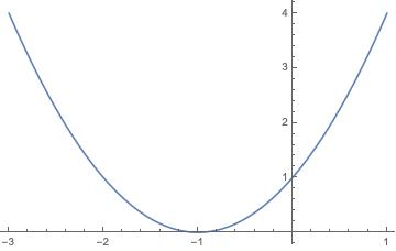
(b) Case 2: Minimizer is out of Figure 1: Different Cases for the Minimizers of Strictly Convex Functions With above remark in our minds, first order conditions are calculated and minimizers are found as:
(4.5) (4.6) In order to solve the 2-equation system, we plug into the equation of and have:
(4.7) The number of solutions of this equation depends on . Since we have and , it is concluded that and we have 2 real-valued solutions. When they are analyzed further, it can be seen that in one of the solutions, and in the other solution .
The set of positive solutions for and are as following:
(4.8) (4.9) In Figure 2, plots of and under different and values can be found.
Figure 2: Control of Major Players under Different and Values - 2.
Solution of the Constrained Optimization Problem of Minor Player. In this section, with given controls for major players and the distribution of other minor players, we are solving the mean field game formulation of the optimization problem of minor players. Our goal is to find the mapping for the control of minor player that minimizes their cost function s.t.:
(4.10) where and denote the control of major players, denotes the mean of the distribution of other minor players’ control and random denotes the initial preference rate of the minor player. Here, the control of minor player is a feedback function depending on their initial position, therefore in the cost function it is going to be denoted as . The function that we want to minimize is as following:
Since the control of minor player is a feedback function, minimizing the integral can be done through minimizing the integrand. In other words, if we denote:
(4.11) Then:
Now, we focus on minimizing (4.11). Since this function is strictly convex in , we may have three different cases for the minimizer as in Figure 3 given . If the first order condition gives a minimizer that is smaller than 0 then the function is minimized at ; on the other hand, if the first order condition gives a minimizer that is bigger than 1, then the function is minimized at , and in the other case, minimizer is found by first order condition.
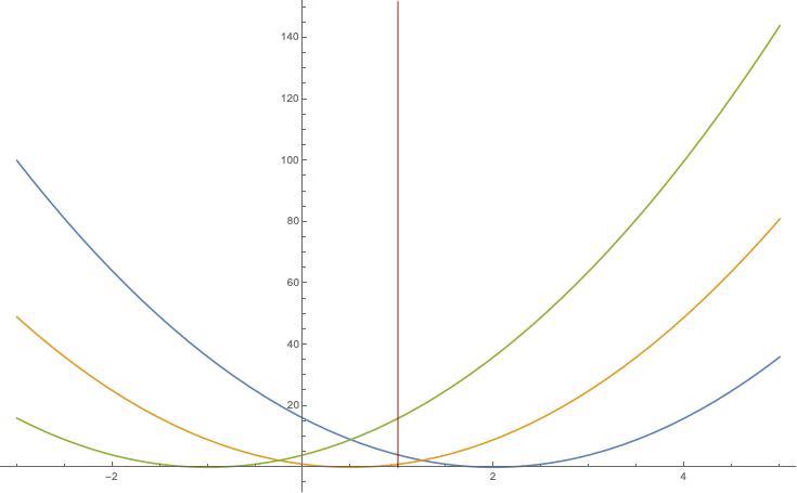
Figure 3: Different Possible Cases fo the Minimizers with Constraint .
When the first order condition is checked the minimizer is found to be:
(4.12) Now, we move to the fixed point argument part such that:
(4.13) Now, we assume that there exists such that . Further we define following sets:
with the following probability measures.
Intuitively this means that given , there may exist some that makes the expression smaller than 0 or bigger than 1 and their probability mass is given as and , respectively. With this assumption the fixed point argument gives us:
(4.14) - 3.
Solution of the System.
Lemma 4.2.
For any given , we have that
(4.15) In other words, we have .
Proof of Lemma 4.2.
First, we realize that any given , the sign of depends on . If , we have . Furthermore, if , we have .
First, we assume that . Then we have , by contradiction we find that .
Secondly, we assume that . In this case, we have and there does not exist that gives . Therefore, we conclude that . Now we focus on . If , it means that there exists some that gives . From here we see that should be bigger than 1.5 and . By using equation (4.14), we have:
Here since and and , we have a contradiction. Therefore, we also conclude that .
Finally, we assume that . In this case, we have and there does not exist that gives . Therefore, we conclude that . Now we focus on . If , it means that there exists some that gives . From here we see that should be smaller than -1.5 and . By using equation (4.14), we have:
Since and , we have a contradiction. Therefore, we also conclude that
∎
By using Lemma 4.2, we can calculate and the final system becomes:
(4.16) where the unit cost of advertisement, , and the distribution of the initial control of minor players, , are given.
∎
Theorem 4.3.
There is a unique Nash Equilibrium in the Mean Field Game with Multiple Major Players.
Proof of Theorem 4.3.
Since the system given in (4.16) gives the Nash Equilibrium solution in the Mean Field Game with Multiple Major Players it is enough to show that the system has a unique solution. If the 3-equation system in (4.16) has a solution, we can conclude that there is existence of the solution to this game.
The existence of the solution of this system can be showed by plugging in and values in the equation for . For any cost of advertisement , we can see that for , there exists a such that and for , there exists a such that . Further we realize that if , we have for any cost of advertisement.
In order to show the uniqueness, we need to show that there is a unique fixed point for . Realize that after plugging in and values can be found by solving the following equation:
If we show that is strictly increasing or decreasing in where , the solution is unique. Therefore, we check the derivative of :
Since and we have , and . Therefore, is strictly increasing which concludes the uniqueness of the fixed point for . Since we previously showed that and are determined uniquely for any given , we conclude that we have a unique Nash equilibrium.
∎
4.2 Multi-Leader-Follower Nash Equilibrium in Mean Field Game with Major Players
In this setting, major players are playing a two-player game assuming that minor players are rational and constructing a Nash Equilibrium among themselves by taking into account the Mean Field Game Equilibrium of the minor players. Here, major players are in a sense Stackelbergian; however, we don’t have a sequential game, major and minor players are giving their responses still simultaneously. At the end Multi-Leader-Multi-Follower Nash Equilibrium is found.
- 1.
We assume that major players think minor players are rational and constructing a Nash Equilibrium among themselves. We take major players’ 2-player game equilibrium controls as and .
- 2.
We fix , and assume that minor players are giving the best response to the controls of major players:
-
By considering the limit , we solve the following mean field game problem for the representative Minor Player, where is the initial control of the minor player which is random:
- –
We find
(4.17)
- –
-
We apply Fixed Point Argument: Find
-
- 3.
Given the MFG equilibrium of minor players, , we solve 2-player game of Major Players:
-
First, we find best response of major player as a function of the other major player’s control:
- –
For major player 1, find
(4.18) - –
For major player 2, find
(4.19)
- –
-
Then we solve the 2-equation system of and to find the equilibrium controls of major players in the 2-player game.
-
- 4.
Finally we have a solution of the following form:
(4.20)
Proposition 4.4.
The final system for the Multi-Leader-Follower Nash Equilibrium in our model is given as
| (4.21) | ||||
where
Proof of Proposition 4.4.
Here, the Mean Field Game solution of the minor player stays the same, remember that we have the following minimizer for the cost function of the minor player:
| (4.22) |
By using the fixed point argument we find
| (4.23) |
where and are defined as in proof of Proposition 4.1.
After, this is plugged into the cost functions of major players, firstly it is checked whether the cost functions of major players are strictly convex in their own controls. Since for the Second Order Condition we have SOC, it is concluded that, cost function of major player 1 (4.18) is strictly convex in and cost function of major player 2 (4.19) is strictly convex in . After first order condition is checked, it is concluded that we have the following minimizers:
| (4.24) | ||||
Lemma 4.5.
For any given , we have that
| (4.25) |
In other words, we have .
Proof of Lemma 4.5.
First we realize that since , given , we cannot have and simultaneously. Therefore, we look at two cases and show contradictions in these cases.
First we assume that . In this case, when the two player system of major players in 4.27 is solved, we realize given any and , we have . Since , we conclude that for all ; therefore, we conclude that which contradicts with our initial assumption.
Secondly, we assume that . In this case, when the two player system of major players in 4.27 is solved, we realize given any and , we have . Since , we conclude that for all ; therefore, we conclude that which contradicts with our initial assumption. ∎
By using Lemma 4.5, we conclude that:
| (4.26) |
Further again by using Lemma 4.5, we can rewrite the minimizers for the major players’ cost functions as follows:
| (4.27) | |||
Now, the 2-equation system (4.27) needs to be solved in order to find the equilibrium. When the solutions are checked, we saw that there exist 2 sets of solutions; one positive and one negative set. Because of the nonnegativity assumption in the controls of the major players, we conclude that the positive set gives the unique optimal control for the major players. ∎
Theorem 4.6.
There exists a unique Multi-Leader-Follower Nash Equilibrium.
5 Experiment Results
5.1 NE: Experiments and Intuitive Remarks
The solution of the above equation system (4.16), , and , are given in the plots (Figure 4, 5, and 6).
First we interpret the results related to the market shares. (Figure 4) From the results, we can infer that at any level of unit cost of advertisement, , and initial market share (mean of initial control of minor players), , market shares of companies become closer. In other words is closer to 0.5 than . Secondly, we can see that this effect is higher when unit cost of advertisement is lower. This is because at lower levels of , both companies are advertising heavily and they affect the marginalized customers on each end. As unit cost of advertisement increases, this effect is less prevalent and market share of product 1 settles down at . On the other hand, if the cost of advertisement, , goes to 0, market becomes perfectly shared, in other words as . Finally, we infer that if at the beginning, the market starts perfectly shared (ie. ) it stays in that way (ie. ).
Now we can focus on the interpretation of the results related to the equilibrium advertisement efficiencies (Figure 5 and 6). As expected at any initial market share () level, as the unit cost of advertisement increases, major players are advertising less because of the high costs. In other words, when , and goes to 0.
Secondly, since the cost functions of major players are the same, symmetric behaviour is observed. In other words, at the same level of unit cost of advertisement, companies are advertising the same amount if they start at the same level of market share. Following this, if the market is shared perfectly initially (), both major players have the same advertisement efficiency level; in other words at the equilibrium.
Furthermore, we realize that at every cost of unit advertisement, as initial market share of product 1 () increases, decreases slightly and increases slightly. The explanation as follows: Since the market share of Product 1 is increasing with , Company 1 decides on smaller advertisement efficiency level when its market share is larger; in other words, gets smaller. This result is in the same direction with the findings in [Doyle, 1968]. On the other hand, since the initial market share for Product 2 is smaller, Company 2 decides to have larger advertisement efficiency level, in order to be able to persuade customers of the opposing company.
Finally, we note that there is no Nash Equilibrium, where market share becomes polarized. In other words, for any and , having or is not a Nash equilibrium. Further, there is no Nash Equilibrium, where companies are not advertising. In other words, for any having and/or is not a Nash Equilibrium.
5.2 MLF-NE:Experiments and Intuitive Remarks
In this section, we interpret the results of the Multi-Leader-Follower Nash Equilibrium. (Figure 7, 8 and 9) First, we note that the same intuitive remarks given in Subsection 5.1 hold for the results. We can summarize them briefly here: 1) The market becomes more homogenized at the equilibrium and this homogenization effect is more prevalent when the cost of advertisement is lower. 2) The behavior of companies are symmetric. If the initial market shares are the same, they advertise the same amounts. 3) At every cost of unit advertisement, as the initial market share of a company increases, its advertising level decreases. 4) There is no Multi-Leader-Follower Nash Equilibrium, where market shares become polarized or where companies are not advertising.
6 Comparison of Nash Equilibrium and Multi-Leader-Follower Nash Equilibrium
We analyzed the different equilibrium behavior (NE & MLF-NE) under different initial market share and cost of advertisement choices in Subsections 5.1 and 5.2. In this part of the report, differences and similarities between standard Nash Equilibrium (NE) and the Multi-Leader-Follower Nash Equilibrium (MLF-NE) are going to be stated. Firstly, we need to emphasize again that the Multi-Leader-Follower Nash equilibrium does not give the Nash Equilibrium among all the players in the classical sense. It gives an Stackelbergian-like equilibrium; therefore, we end up with different results.
As stated above in Subsections 5.1 and 5.1, both equilibrium points have some similarities. For example, major players’ advertisement efficiency decisions are moving in the same direction in both of the equilibrium notions under the changes in unit cost of advertisement, , or initial market share, . For example, in both cases, major players are advertising less when is higher. Moreover, in both of the equilibrium notions, market shares become closer and if the unit cost of advertisement goes to infinity, goes to .


As there are some similarities in the equilibrium results, there are also differences. In Figure 10, we can see the control chosen by the Major Player 1, in the Nash Equilibrium (left) and in the Multi-Leader-Follower Nash Equilibrium (middle) given different unit cost of advertisement, and initial market share, values. In order to compare them, we also plot the difference of the controls chosen by the Major Player 1 in two different equilibria (right). In this 3D plot, we can see that this difference is positive. Therefore, we note that companies are advertising less in the Multi-Leader-Follower Nash Equilibrium at every level of unit cost of advertisement, and initial market share, . However, this difference is more significant at the lower levels of . In other words, in Nash Equilibrium solution there is excessive advertisement (Figure 10 and 11). Consequently, when the total cost is analysed, it is seen that companies are having a higher cost in the Nash Equilibrium. However this difference is getting insignificant as unit cost of advertisement increases (Figure 12). Finally, even if in both cases market shares become closer ( is closer to 0.5 than ), it is seen that in Nash Equilibrium solution if then also . However, in the Multi-Leader-Follower Nash Equilibrium solution, it can be seen that at the lower levels of the unit cost of advertisement, we end up with when . This means that if the cost of advertisement is small enough, in MLF-NE, companies in an adverse position initially have a chance to be the leader of the market with advertising. (Figure 13)

In conclusion, since companies are advertising significantly higher in Nash Equilibrium at the lower levels of , they are ending up with a significantly higher total cost. Therefore, it can be concluded that it would be the best for companies if they can understand the consumers’ behavior and play a 2-player game with the opponent company.
7 Conclusion
In this paper, we analysed two different equilibrium notions for the advertising competition game in a duopoly market when consumers are involved. In the first equilibrium notion (NE), Nash equilibrium is found among all players including major and minor players; on the other hand, in the second equilibrium notion (MLF-NE), major player is assuming minor players are rational and constructing a Nash equilibrium among themselves and they are playing a 2-player game with the opposing company. In this paper, since we have a large number of consumers, mean field game approximation is used in order to find the Nash equilibrium of the minor players. After models are constructed, solution methodologies are given and it is concluded that there exists a unique solution in both cases. Finally, the solutions are compared and it is recommended to the companies in the duopoly to understand the behavior of consumers and use the MLF-NE solution. In this way, they have smaller total costs in the equilibrium by evading from unnecessary levels of advertisement.
Main contribution of this report is using the multiple major players and minor players mean field games methodology on the advertisement competition of a duopoly. Even if the model is designed as a static (one-shot) game, the extension to the dynamic version is planned as a future work.
Acknowledgments. We would like to thank Dr. Mathieu Lauriere for his valuable comments on the manuscript. Furthermore, we thank the anonymous referee for their valuable feedback that helped us to clarify and improve this manuscript.
References
- [Bass et al., 2005] Bass, F. M., Krishnamoorthy, A., Prasad, A., and Sethi, S. P. (2005). Generic and brand advertising strategies in a dynamic duopoly. Marketing Science, 24(4):556–568.
- [Bensoussan et al., 2016] Bensoussan, A., Chau, M. H. M., and Yam, S. C. P. (2016). Mean field games with a dominating player. Applied Mathematics & Optimization, 74(1):91–128.
- [Carmona and Delarue, 2013] Carmona, R. and Delarue, F. (2013). Probabilistic analysis of mean-field games. SIAM Journal on Control and Optimization, 51(4):2705–2734.
- [Carmona and Delarue, 2018] Carmona, R. and Delarue, F. (2018). Probabilistic theory of mean field games with applications. Springer.
- [Carmona and Wang, 2017] Carmona, R. and Wang, P. (2017). An alternative approach to mean field game with major and minor players, and applications to herders impacts. Applied Mathematics & Optimization, 76(1):5–27.
- [Carmona and Zhu, 2016] Carmona, R. and Zhu, X. (2016). A probabilistic approach to mean field games with major and minor players. Ann. Appl. Probab., 26(3):1535–1580.
- [Chan and Sircar, 2015] Chan, P. and Sircar, R. (2015). Bertrand and cournot mean field games. Applied Mathematics & Optimization, 71(3):533–569.
- [Clarke, 1973] Clarke, D. G. (1973). Sales-advertising cross-elasticities and advertising competition. Journal of Marketing Research, 10(3):250–261.
- [Doyle, 1968] Doyle, P. (1968). Advertising expenditure and consumer demand. Oxford Economic Papers, 20(3):394–416.
- [Erickson, 1995] Erickson, G. M. (1995). Differential game models of advertising competition. European Journal of Operational Research, 83(3):431 – 438.
- [Fruchter, 1999] Fruchter, G. E. (1999). Oligopoly advertising strategies with market expansion. Optimal Control Applications and Methods, 20(4):199–211.
- [Fruchter and Kalish, 1997] Fruchter, G. E. and Kalish, S. (1997). Closed-loop advertising strategies in a duopoly. Management Science, 43(1):54–63.
- [Garella and Petrakis, 2008] Garella, P. G. and Petrakis, E. (2008). Minimum quality standards and consumers’ information. Economic Theory, 36(2):283–302.
- [Hattori and Higashida, 2012] Hattori, K. and Higashida, K. (2012). Misleading advertising in duopoly. The Canadian Journal of Economics / Revue canadienne d’Economique, 45(3):1154–1187.
- [Hu and Fukushima, 2015] Hu, M. and Fukushima, M. (2015). Multi-leader-follower games: Models, methods and applications. Journal of the Operations Research Society of Japan, 58(1):1–23.
- [Huang et al., 2004] Huang, M., Caines, P. E., and Malhamé, R. P. (2004). Large-population cost-coupled lqg problems: generalizations to non-uniform individuals. In Decision and Control, 2004. CDC. 43rd IEEE Conference on, volume 4, pages 3453–3458. IEEE.
- [Huang et al., 2006] Huang, M., Malhamé, R. P., and Caines, P. E. (2006). Large population stochastic dynamic games: closed-loop mckean-vlasov systems and the nash certainty equivalence principle. Commun. Inf. Syst., 6(3):221–252.
- [Huang et al., 2003] Huang, M., Pe, C., and Malhame, R. (2003). Individual and mass behaviour in large population stochastic wireless power control problems: centralized and nash equilibrium solutions. In 42nd IEEE International Conference on Decision and Control (IEEE Cat. No.03CH37475), volume 1, pages 98–103.
- [Lasry and Lions, 2007] Lasry, J.-M. and Lions, P.-L. (2007). Mean field games. Japanese Journal of Mathematics, 2(1):229–260.
- [Mankiw, 2012] Mankiw, N. G. (2012). Principles of Microeconomics. South-Western Cengage Learning, sixth edition edition.
- [Nourian and Caines, 2013] Nourian, M. and Caines, P. (2013). -nash mean field game theory for nonlinear stochastic dynamical systems with major and minor agents. SIAM Journal on Control and Optimization, 51(4):3302–3331.
- [Prasad and Sethi, 2003] Prasad, A. and Sethi, S. (2003). Dynamic optimization of an oligopoly model of advertising.
- [Prasad and Sethi, 2004] Prasad, A. and Sethi, S. P. (2004). Competitive advertising under uncertainty: A stochastic differential game approach. Journal of Optimization Theory and Applications, 123(1):163–185.
- [Salhab et al., 2016] Salhab, R., Malhame, R., and Ny, J. L. (2016). A dynamic collective choice model with an advertiser. IEEE 55th Conference on Decision and Control (CDC).
- [Singh and Vives, 1984] Singh, N. and Vives, X. (1984). Price and quantity competition in a differentiated duopoly. The RAND Journal of Economics, 15(4):546–554.
- [Vidale and Wolfe, 1957] Vidale, M. and Wolfe, H. (1957). An operations-research study of sales response to advertising. Operations research, 5(3):370–381.