Equivalence between fermion-to-qubit mappings in two spatial dimensions
Abstract
We argue that all locality-preserving mappings between fermionic observables and Pauli matrices on a two-dimensional lattice can be generated from the exact bosonization in Ref. Chen et al. 2018, whose gauge constraints project onto the subspace of the toric code with emergent fermions. Starting from the exact bosonization and applying Clifford finite-depth generalized local unitary (gLU) transformation, we can achieve all possible fermion-to-qubit mappings (up to the re-pairing of Majorana fermions). In particular, we discover a new super-compact encoding using 1.25 qubits per fermion on the square lattice, which is lower than any method in the literature. We prove the existence of fermion-to-qubit mappings with qubit-fermion ratios for positive integers , where the proof utilizes the trivialness of quantum cellular automata (QCA) in two spatial dimensions. When the ratio approaches 1, the fermion-to-qubit mapping reduces to the 1d Jordan-Wigner transformation along a certain path in the two-dimensional lattice. Finally, we explicitly demonstrate that the Bravyi-Kitaev superfast simulation, the Verstraete-Cirac auxiliary method, Kitaev’s exactly solved model, the Majorana loop stabilizer codes, and the compact fermion-to-qubit mapping can all be obtained from the exact bosonization.
I Introduction
A fermion-to-qubit mapping is a duality between local even11 1 We only consider terms respecting the fermion-parity symmetry, i.e., products with even numbers of fermionic creation and annihilation operators. fermionic operators and local products of Pauli matrices. It is well known that any fermionic system in a 1d lattice can be mapped onto a 1d spin system by the Jordan-Wigner transformation. The Jordan-Wigner transformation can also be applied to systems in higher dimensions by choosing a particular ordering of fermions; however, the mapping becomes highly non-local. From both theoretical and practical points of view, mapping local fermionic operators to local spin operators in higher dimensions is an essential topic. In the last two decades, there have been many proposals of fermion-to-qubit mappings for two dimensions Verstraete and Cirac 2005; Kitaev 2006; Whitfield et al. 2016; Chen et al. 2018; Jiang et al. 2019; Setia et al. 2019; Bochniak and Ruba 2020; Derby et al. 2021; Po 2021 and three or arbitrary dimensions Bravyi and Kitaev 2002; Chen and Kapustin 2019; Chen 2020. These fermion-to-qubit mappings play important roles in various topics of modern physics, such as exactly solvable models for topological phases Kitaev 2006; Ellison and Fidkowski 2019; Chen et al. 2021; Chen and Hsin 2021, fermionic quantum simulations Bravyi and Kitaev 2002; Verstraete and Cirac 2005; Whitfield et al. 2016; Jiang et al. 2019; Derby et al. 2021, and quantum error correction Bravyi et al. 2010; Vijay and Fu 2016; Viyuela et al. 2019; Vijay et al. 2015; Litinski and von Oppen 2018; Hastings 2017. In particular, the exact bosonizations in Refs. Chen et al. 2018; Chen and Kapustin 2019; Chen 2020; Bochniak and Ruba 2020 construct the toric code with fermions in arbitrary dimensions and impose gauge constraints to restrict in the subspace with emergent fermions, which provide an elegant spacetime description by the Chern-Simons and the Steenrod square topological action. The spacetime pictures for other fermion-to-qubit mappings mentioned above are not manifest. Ref. Whitfield et al. 2016 points out that the Verstraete-Cirac auxiliary method Verstraete and Cirac 2005 can be related to a topological model (toric code), and the compact encoding Derby et al. 2021 found that its stabilizer is similar to a toric code.
From the theoretical perspective, it is tempting to ask a question: are all fermion-to-qubit mappings in two spatial dimensions “equivalent” to the exact bosonization? First, we define the “equivalence” by finite-depth generalized local unitary (gLU) transformations. Informally speaking, finite-depth gLU transformation is a finite-depth quantum circuit (FDQC) with ancilla qubits. We argue that the answer to the above question is “yes” and demonstrate it with examples.
From the practical point of view, fermion-to-qubit mappings are widely used in fermionic quantum simulations of physical systems. In practical quantum simulations, an important quantity is the qubit-fermion ratio , the number of qubits to simulate one fermion on average, since it is directly related to the total number of fermionic modes encoded in a qubit array. Suppose we encode fermionic modes by qubits, then the qubit-fermion ratio is . The best fermion-to-qubit mapping on the 2d square lattice is the compact fermion-to-qubit mapping with the ratio Derby et al. 2021.
In this work, we focus on lattices in two spatial dimensions. First, we construct a new super-compact fermion-to-qubit mapping with the qubit-fermion ratio on the 2d square lattice. Moreover, we provide a systematic approach to construct various 2d bosonizations by utilizing the ideas of Clifford circuit Gottesman 1998a; Gottesman 1998b and finite-depth generalized local unitary (gLU) transformations Chen et al. 2010; Zeng et al. 2018. Such an approach provides a new perspective to study the relationship between different fermion-to-qubit mappings. We find that all the local fermion-to-qubit mappings can be generated from the exact bosonization by finite-depth gLU transformations. In particular, we explicitly show how to obtain the Bravyi-Kitaev superfast encoding (BKSF), the Verstraete-Cirac mapping, Kitaev’s honeycomb model, the Majorana loop stabilizer codes (MLSC), and the compact fermion-to-qubit mapping.
Summary of results
We first demonstrate a super-compact fermion-to-qubit mapping on the 2d square lattice with qubit-fermion ratio in Sec. II and compare its data with other fermion-to-qubit mappings in Table 1. In Sec. III, we define the crucial theoretical technique in our construction: the generalized local unitary (gLU) transformation Chen et al. 2010; Zeng et al. 2018. Then, in Sec. III.2, we derive the fermion-to-qubit mapping, which is equivalent to the compact encoding Derby et al. 2021. In Sec. III.3, we further improve the ratio to derive the construction shown in the previous section. In Sec. III.4, we prove that a general construction with ratio exists for any positive integer . The proof utilizes the trivialness of 2d quantum cellular automata (QCA) Freedman and Hastings 2020; Haah 2021a. In Sec. IV, we define the equivalence relation between different 2d bosonizations based on finite-depth gLU transformations and discuss the equivalence between the exact bosonization and many well-known fermion-to-qubit mappings. We construct explicit Clifford circuits that convert the exact bosonization to the Bravyi-Kitaev superfast encoding (Sec. IV.1), the Verstraete-Cirac mapping (Sec. IV.2), Kitaev’s honeycomb model (Sec. IV.3), the Majorana loop stabilizer codes (Sec. IV.4), and the Jordan-Wigner transformation (Sec. IV.5).
| qubit-fermion-ratio | fermion parity weight | hopping weight | stabilizer weight | |
| Verstraete-Cirac Verstraete and Cirac 2005 22 2 The graph structure of the auxiliary Hamiltonian is Fig. 15. | 2 | 1 | 3-4 | 6 |
| BKSF Bravyi and Kitaev 2002 33 3 The ordering of edges is shown in Fig. 14. | 2 | 4 | 2-6 | 6 |
| Kitaev’s honeycomb model Kitaev 2006 | 2 | 2 | 2-5 | 6 |
| Exact bosonization Chen et al. 2018 | 2 | 4 | 2-6 | 6 |
| MLSC Jiang et al. 2019 | 2 | 3 | 3-4 | 4-10 |
| Compact fermion-to-qubit mapping Derby et al. 2021 | 1.5 | 1 | 3 | 8 |
| Super-compact fermion-to-qubit mapping | 1.25 | 1-2 | 2-6 | 12 |
II Super-compact fermion-to-qubit mapping
In this section, we introduce a super-compact encoding of fermions by qubits with the qubit-fermion ratio . We first introduce the Hilbert spaces for fermions and qubits and then describe the mapping between them.
On the 2d square lattice in Fig. 2, each vertex contains a fermionic mode with creation/annihilation operator , with the standard commutation relation . It is easier to use the Majorana basis
| (1) |
The local fermion parity operator at a vertex is
| (2) |
and the hopping operator on an edge is
| (3) |
where and are the left and right vertices of the edge defined in Fig. 1. The even algebra of fermions consists of local observables with a trivial fermion parity, i.e., local observables which commute with the total fermion parity .44 4 The even fermionic algebra can also be considered as the algebra of local observables containing an even number of Majorana operators. The generators for the even algebra of fermions are and on all edges and vertices Chen et al. 2018.


On the other hand, the qubits are put at vertices in Fig. 2. We label vertices by black and grey colors. For each black vertex, there is 1 qubit, and for each grey vertex, there are 2 qubits. As shown in Fig. 3 and 4, each grey vertex has two Pauli matrices on the top-right and bottom-left corners respectively.
The fermion-to-qubit mappings are mappings from to Pauli strings (products of Pauli matrices) on qubits with the same algebra. In addition, such mapping satisfies a condition that the product of along an arbitrary closed path should be the identity operator (up to a phase) since all Majorana operators cancel out. Such constraint requires the qubit system to be stabilized by a stabilizer group which is a set of hopping operators along with all closed loops. Now, we explicitly construct the mapping on the lattice in Fig. 2:
| (4) |
where and are defined in Fig. 3. It can be checked that two operators and anti-commute if and only if and are two distinct edges sharing one common vertex, and and anti-commute if and only if the edge contains the vertex . Therefore, and satisfy the same commutation relations. The last step is to impose the stabilizer conditions (gauge constraints) that product of on a loop is proportional to the identity operator:
| (5) |
where is the length of the loop .
The generators of this stabilizer condition are expressed in Fig. 4. The stabilizers for the vertices that connect pink, black, green, purple edges generate the whole stabilizer group. The weight of such a stabilizer is .


III Generalized local unitary circuits on the exact bosonization

We describe a systematical way to derive fermion-to-qubit mappings from the exact bosonization in two spatial dimensions in the section. In Ref. Chen et al. 2018, the exact bosonization is proposed using the subspace of the toric code with fermionic excitations, which will be reviewed in Sec. III.1. By applying local unitary operators on the exact bosonization, we can generate a new fermion-to-qubit mapping. However, to include the lattice deformation or changing of the Hilbert spaces, local unitary operators are not sufficient, and the idea of generalized local unitary (gLU) operators is introduced.
The generalized local unitary (gLU) Chen et al. 2010; Zeng et al. 2018 arises from the idea of wave function renormalization where local unitary operators are used to add or remove degrees of freedom at different length scales. For a wave function, we can use an operation to add or remove ancilla qubits in the product state.55 5 Since the ancilla qubits are in the products, adding or removing them do not change the information contained in the state. We call the transformation that changes the degrees of freedom a generalized local unitary (gLU) operator. The formal definition of gLU in Ref. Chen et al. 2010 is as follows. For a quantum state with the reduced density matrix in region , only acts in a support subspace of the total Hilbert space . The dimension of is , which is called support dimension. Hence, the total Hilbert space on region can be written as a direct sum . Let , to be the basis of , , to be the basis of , and , to be the basis of (). We introduce the local unitary transformation to rotate to . In the new basis, wave function only has non-zero amplitudes on the first basis vectors, and therefore we can truncate out the remaining columns of to get the gLU operator without losing any information.
With gLU transformation, we can remove the degrees of freedom in the system if they are in the product states. This operation is equivalent to disentangling parts of qubits from others. Hence, the qubit-fermion ratio can be improved by wisely applying finite-depth gLU to the exact bosonization. In this paper, we will use finite-depth gLU Clifford circuits since we focus on Pauli stabilizer models. We demonstrate the construction of fermion-to-qubit mappings with ratio in Sec. III.2 and in Sec. III.3 by conjugating the 2d exact bosonization by certain finite-depth gLU Clifford circuits.
III.1 Review of the exact bosonization
We review the exact bosonization on the Hilbert space defined in Fig. 6. The elements of vertices, edges, and faces are denoted . On each face of the lattice we place a single pair of fermionic creation-annihilation operators , or equivalently a pair of Majorana fermions . The even fermionic algebra consists of local observables with a trivial fermion parity, i.e., local observables which commute with the total fermion parity . The even algebra is generated by Chen et al. 2018:
- 1.
On-site fermion parity:
(6) - 2.
Fermionic hopping term:
(7) where and are faces to the left and right of , with respect to the orientation of in Fig. 6.
The bosonic dual of this system involves -valued spins on the edges of the square lattice. For every edge , we define a unitary operator that squares to . Labeling the faces and vertices as in Fig. 6, we define:
| (8) |
where , are Pauli matrices acting on a spin at each edge . Operators for other edges are defined by using translation symmetry. Pictorially, the operator is drawn as
| (9) |
corresponding to the vertical or horizontal edge .
It has been shown in Ref. Chen et al. 2018 that and satisfy the same commutation relations. We also map the fermion parity at each face to the “flux operator” , the product of around a face :
| (10) |
The bosonization map is
| (11) |
or pictorially
The condition on fermionic operators gives gauge constraints (stabilizer) for bosonic operators, or generally
| (40) |
The gauge constraint Eq. (40) can be considered as the stabilizer ( for in the code space), which forms the stabilizer group . The operators and generate all logical operators.66 6 The logical operators consist of all operators that commute with . are trivial logical operators since stabilizers have no effect on the code space. and generate all logical operators. In the setting above, qubits live on edges and fermions live on faces, so the ratio between the number of qubits and the number of fermions is . We are going to apply finite-depth gLU transformations to lower this ratio.
III.2 Compact fermion-to-qubit mapping with ratio
In the exact bosonization on the square lattice, the bosonic subspace is constrained by the stabilizer Eq. (40) at each vertex. First, we enlarge the unit cell to be a square
| (41) |
Note that we have colored the faces to be even or odd as the checkerboard. In each square, there are totally fermions, qubits and stabilizers, whose qubit-fermion ratio is . We are going to apply a finite-depth gLU circuit to disentangle some qubits and reduce the ratio.
In Fig. 7, the translational invariant Clifford circuit is defined.77 7 We have enlarged the unit cell and therefore the distances for the translational generators are doubled. We divide the stabilizers into two cases, living on an odd face or an even face, as shown below
After the conjugation of the Clifford circuit in Fig. 7, these stabilizers become
We have converted the stabilizer into a single-qubit stabilizer . This qubit will be in the eigenstate of and can be discarded. Hence, we successfully eliminate the qubits on the left edges of all odd faces. In the unit square Eq. (41), there are only 6 qubits remaining, and the ratio between qubits and fermions is .
By the Clifford circuits in Fig. 7, we eliminate stabilizers on odd faces and convert the stabilizers on even faces to toric-code-like stabilizers. Next, we analyze the logical operators which represent the hopping of fermion after the conjugation. Here the convention of the fermionic hopping is . There are four types of fermionic hopping operator (after removing the degrees of freedom in Eq. (III.2))
| (72) |
and two types of flux operators
| (73) |
We note that the stabilizer in Eq. (III.2) is the same as the stabilizer of the compact encoding in Ref. Derby et al. 2021 (up to the relabeling of Pauli matrices , , ). Since the stabilizers are the same, the space of logical operators must be equivalent. We can redefine the bottom two lines of Eq. 72 as “fermion parity” by re-pairing of Majorana fermions as Fig. 8, and reproduce the compact encoding in Ref. Derby et al. 2021.

III.3 Super-compact fermion-to-qubit mapping with ratio

Based on the construction in the previous section, which is obtained from conjugating the original 2d bosonization by the Clifford circuit shown in Fig. 7, we further conjugate it by the Clifford circuit in Fig. 10. In the construction, we label squares by “even” and “odd”. Since the translational invariant Clifford circuit in Fig. 10 acts on a cell, we color squares by 4 different colors: yellow, blue, red, and green and call them class 1, 2, 3, and 4 squares. Classes 1 and 3 belong to “odd” faces, while classes 2 and 4 belong to the “even” faces.


Conjugated by the circuits in Fig. 10, the stabilizers enveloping blue and yellow squares become
However, the stabilizers enveloping green and red squares become
which is trivial. Then, we can simply remove the qubits on the boundaries between yellow and blue squares, which reduces the qubit-fermion ratio to .
Similarly, we conjugate Eq. (72) and (73) by the Clifford circuit in Fig. 10, and the result of these logical operators are listed in Fig. 11. This gives the super-compact fermion-to-qubit mapping demonstrated in Sec. II by a re-pairing of Majorana fermions (Fig. 12) and a slight lattice deformation.
III.4 General Construction for compact fermion-to-qubit mappings
In this section, we describe a general method to construct fermion-to-qubit mappings with a reduced qubit-fermion ratio from the exact bosonization. The exact bosonization contains gauge constraints (stabilizers) Eq. (40) supported on faces (northeast to vertices ), and we rename as for convenience. We enlarge the unit cell and will show that it is always possible to apply finite-depth gLU operators such that a portion of stabilizers can be mapped to a single Pauli matrix. More precisely, we are going to prove that the stabilizer on each white face below can be mapped to a single Pauli matrix:
| (74) |
where can be any positive integer.88 8 The portion of grey faces over all faces is . After removing stabilizers on white faces, the qubit-fermion ratio becomes .
Instead of transforming on white faces directly, we are going to prove a stronger statement: the gauge constraints (Eq. (40)) on white faces, the hopping operators (Eq. (IV.3)) across horizontal edges, and the operators
| (75) |
on grey faces, can all be mapped to a single Pauli matrix simultaneously under a finite-depth gLU circuit. These operators on the square lattice are shown as
| (76) |
To prove the above statement, we need to introduce a lemma:
Lemma 1.
Given and for all edges that are products of Pauli matrices on a neighborhood of the edge satisfying the Pauli algebra,
there exists a finite-depth gLU transformation mapping to (a single Pauli on edge ).
Proof.
The (Clifford) quantum cellular automata (QCA) in two spatial dimensions are simply (Clifford) local unitary circuits and shifts Freedman and Hastings 2020; Haah 2021a. The map
| (77) |
defines a QCA and therefore can be decomposed to a Clifford circuit and shifts. For the shift operator, we can introduce ancilla in the states and define the shift operator moving the ancilla in the opposite direction, such that the net flow of qubits is zero. Then, this shift operator can be expressed by a local unitary circuit (involving the ancilla degrees of freedom). In the end, these ancilla are still in the states and can be removed by a finite-depth gLU transformation. Therefore, there exists a finite-depth gLU transformation from to and vice versa. ∎
Lemma 2.
Given operators (separators) and (flippers) that are products of Pauli matrices on a neighborhood of the edge satisfying
| (78) |
there exist operators that are products of Pauli matrices on a neighborhood of edges such that
In other words, if the flippers do not commute with themselves, they can be modified such that the Pauli algebra is satisfied.
Proof.
If and do not commute,
| (79) |
we define
| (80) |
Notice that only affects the commutation relation between and and this fixes the commutation for the part and leaves part unchanged. Therefore, and satisfy the Pauli algebra. ∎
The operators and are call separators and flippers Haah et al. 2018. Once the separators and flippers are given, a QCA is defined by Eq. (77) (after defining by Eq. (80)). By lemma 1, the separator can be mapped to a single Pauli matrix by a finite-depth gLU transformation.
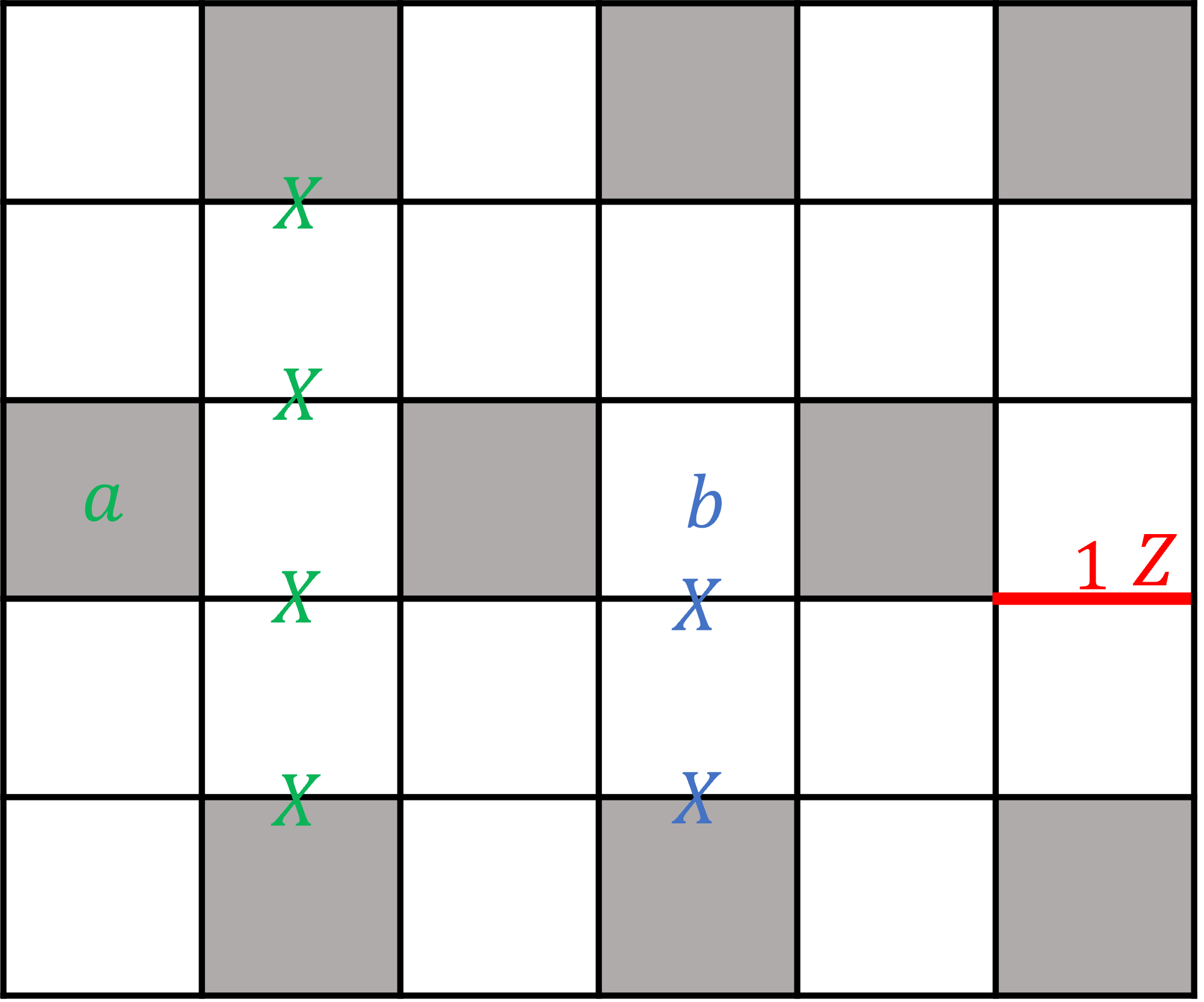
The operators on white faces, on horizontal edges, and in grey faces in (76) are the separators . Now, we are going to describe their flippers:
- 1.
For on grey faces, we define its flippers by the product of (-strings of the toric code) connecting two grey faces on the column to the right, as shown in Fig. 13. It can be checked that this -string only violates exactly one and commute with all other separators and .
- 2.
A potential flipper99 9 The potential flipper is an operator satisfying the algebra (78) partially. For example, it may anti-commute with extra separators . This issue can be fixed by attaching other operators to this potential flipper. for the separator on a white face is the product of connecting the white face to the grey face below (Fig. 13). This operator flips exactly one on white faces and commutes with , but it may anti-commute with a on a grey face. In this case, we can always attach the flipper for this (found in step 1) to the potential flipper. This operator becomes the true flipper for a single .
- 3.
For on a horizontal edge, we start with a potential flipper on this edge . It is obvious that it flips only one and may anti-commute a finite number of and on white and grey faces. Since we have already found the flippers for and , we can attach these flippers to the potential flipper such that the combined operator commutes will all separators except one .
We have found the complete set of separators and flippers on the square lattice. By Lemma 1, the on each white face can be mapped to a single Pauli matrix.
IV Equivalence between fermion-to-qubit mappings and the exact bosonization
In this section, we argue that any locality preserving fermion-to-qubit mappings1010 10 To be precise, we consider the mapping between local fermionic observables and local products of Pauli matrices. in two spatial dimensions can be connected to the exact bosonization by a finite-depth gLU transformation. First, given a fermion-to-qubit mapping, it must contain the flux operators (images of the local fermion parity) and the gauge constraints (images of the product of fermionic hopping terms in a small closed loop). On a torus, we can define a Pauli stabilizer code as
| (81) |
Over two large cycles of the torus, we have the -fold ground state degeneracy since we do not impose the fermionic constraints on the large cycles. The code distance is linear in the system size since the logical operator is the product of hopping along with the large cycles. It is proven in Ref. Haah 2021b that any translationally invariant Pauli stabilizer model with a linear code distance is decomposed by a local Clifford circuit of constant depth into a finite number of copies of the toric code for any prime .1111 11 In this paper, we only work on qubits, which corresponds to . Therefore, the theorem in Ref. Haah 2021b is valid. Since the degeneracy is 4 on the torus, the above stabilizer code Eq. (81) must be a single copy of toric code up to a Clifford circuit. Therefore, and are related to and in the exact bosonization in Sec. III.1 by a gLU transformation (since the toric code defined on different lattice should be related by gLU transformation to add or remove qubits).
In the following part of this section, we will explicitly demonstrate how to transform many well-known fermion-to-qubit mappings in literature to the exact bosonization.
IV.1 Bravyi-Kitaev superfast simulation
The Bravyi-Kitaev superfast simulation (BKSF) in Ref. Bravyi and Kitaev 2002 is a method to encode fermionic operators into Pauli operators. BKSF encodes complex fermions at vertices by qubits on edges . The key idea of BKSF is to assign an arbitrary ordering of edges around each vertex and write down the logical operators according to the ordering. For vertex , we label the edges connected to by , on 2d square lattice, shown in Fig. 14.
The logical operators and are defined as
| (82) |
where is the label of edge on the vertex , is the label of edge on the vertex . The fermion-to-qubit mapping is
| (83) |
where and are fermionic operators defined in Sec. II. The product of on any closed loop need to satisfy the condition Eq. (5) due to the identity for Majorana operators

By the convention in Fig. 14, we have:
| (84) |
We notice that this is the same logical operator as the exact bosonization in the dual lattice after we relabel the Pauli matrices and . The fermion parity terms in both cases are just a product of around a vertex (a face in the dual lattice), and therefore the BKSF approach with this ordering convention is the same as the exact bosonization.
IV.2 Verstraete-Cirac auxiliary method
In this section, we demonstrate the equivalent relation between the Verstraete-Cirac mapping Verstraete and Cirac 2005 and exact bosonization after regrouping Majorana fermions. The basic idea of the Verstraete-Cirac mapping is to eliminate the nonlocal Pauli -string from the 1d Jordan-Wigner transformation by introducing auxiliary qubits with gauge constraints. In this mapping, each site uses four Majorana modes to encodes a complex fermion and an auxiliary complex fermion. For implementation, we put two qubits on each vertex, one for the physical complex fermion, the other for the auxiliary complex fermion. The Majorana operators , belong to the auxiliary complex fermion. The auxiliary fermions stay in the ground state of following Hamiltonian
| (85) |
where the includes only pairs that connected by the directed edges in Fig. 15.
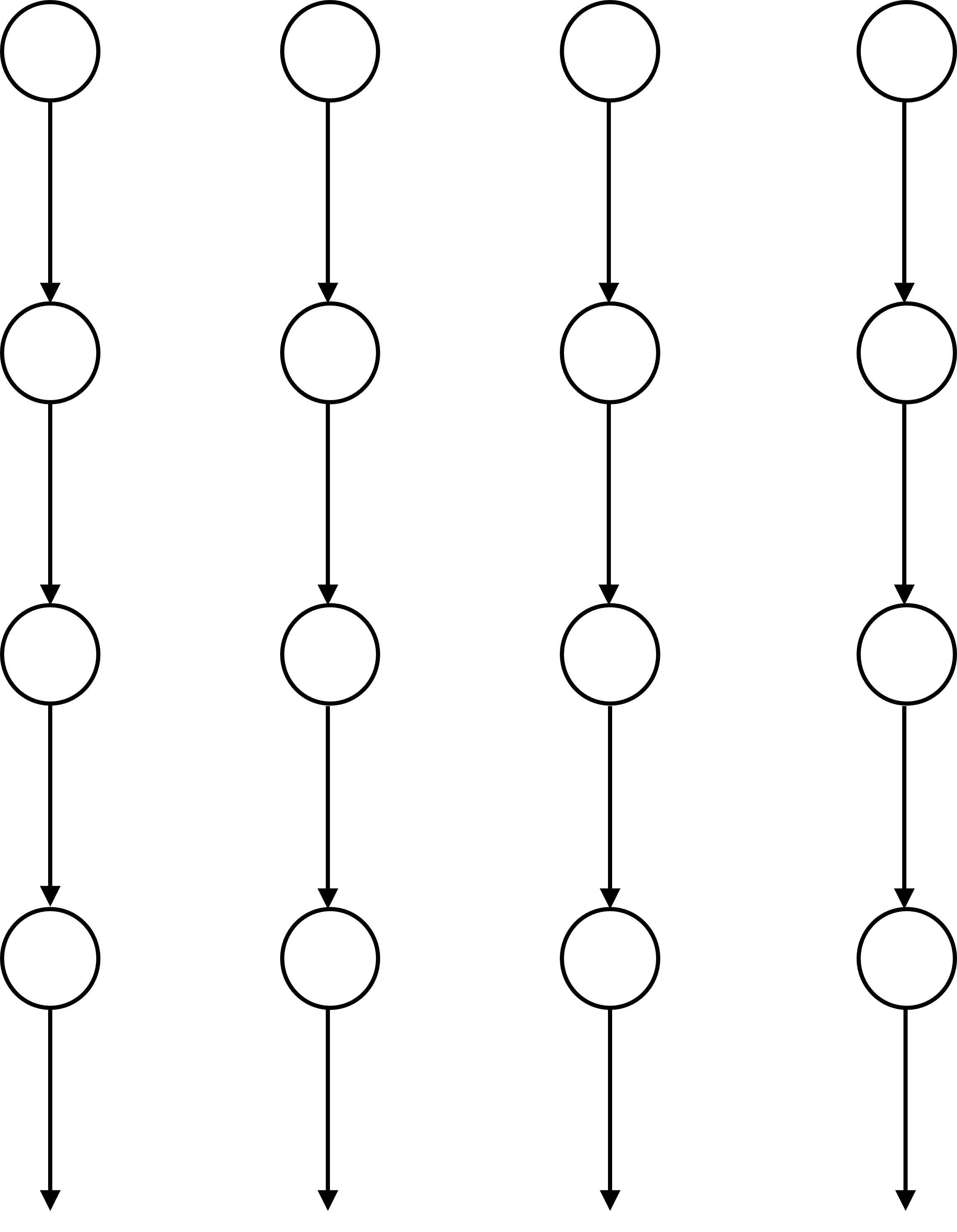
The hopping operator is modified as . We apply the 1d Jordan-Wigner transformation with ordering , where in our convention start with the first row from left to right, and move to the second and so on. However, the auxiliary Hamiltonian is a non-local Hamiltonian. To resolve this problem, we perform following substitution , for all rows. Since all commute with each other, the auxiliary Hamiltonian becomes local without changes in the ground state. Then the local gauge constraint (stabilizer) is . The gauge constraint can be written as a Pauli stabilizer
| (86) |
Pauli matrices act on the auxiliary qubit . We put physical qubits on the vertical edges and auxiliary qubits on the horizontal edges. Since physical qubits and auxiliary qubits are in different edges, we will not show the tilde in following text for convenience.
By conjugating the logical operators in Eq. (87) by the Clifford circuits shown in Fig. 16, the logical operators and stabilizer become
| (88) |

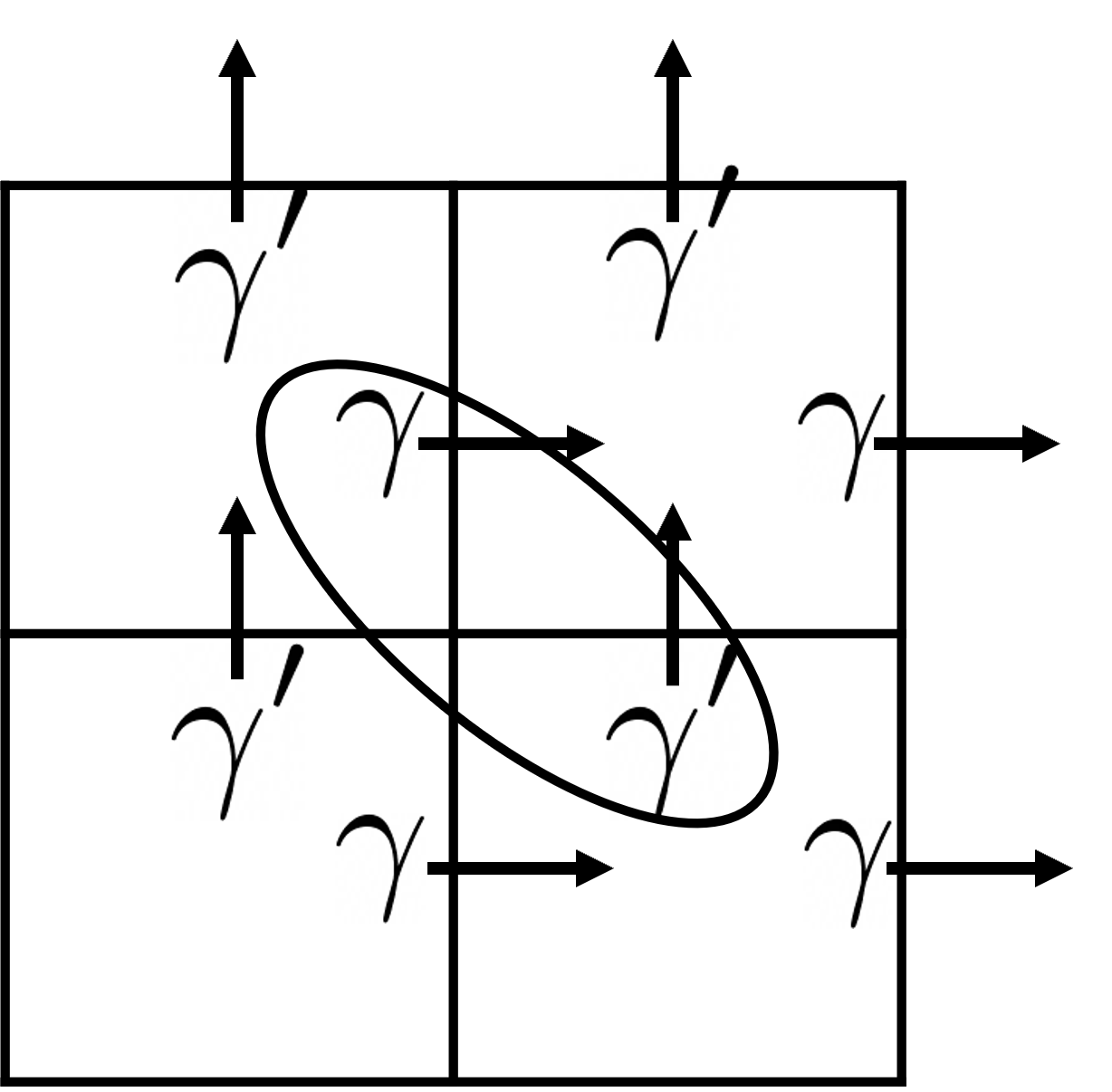
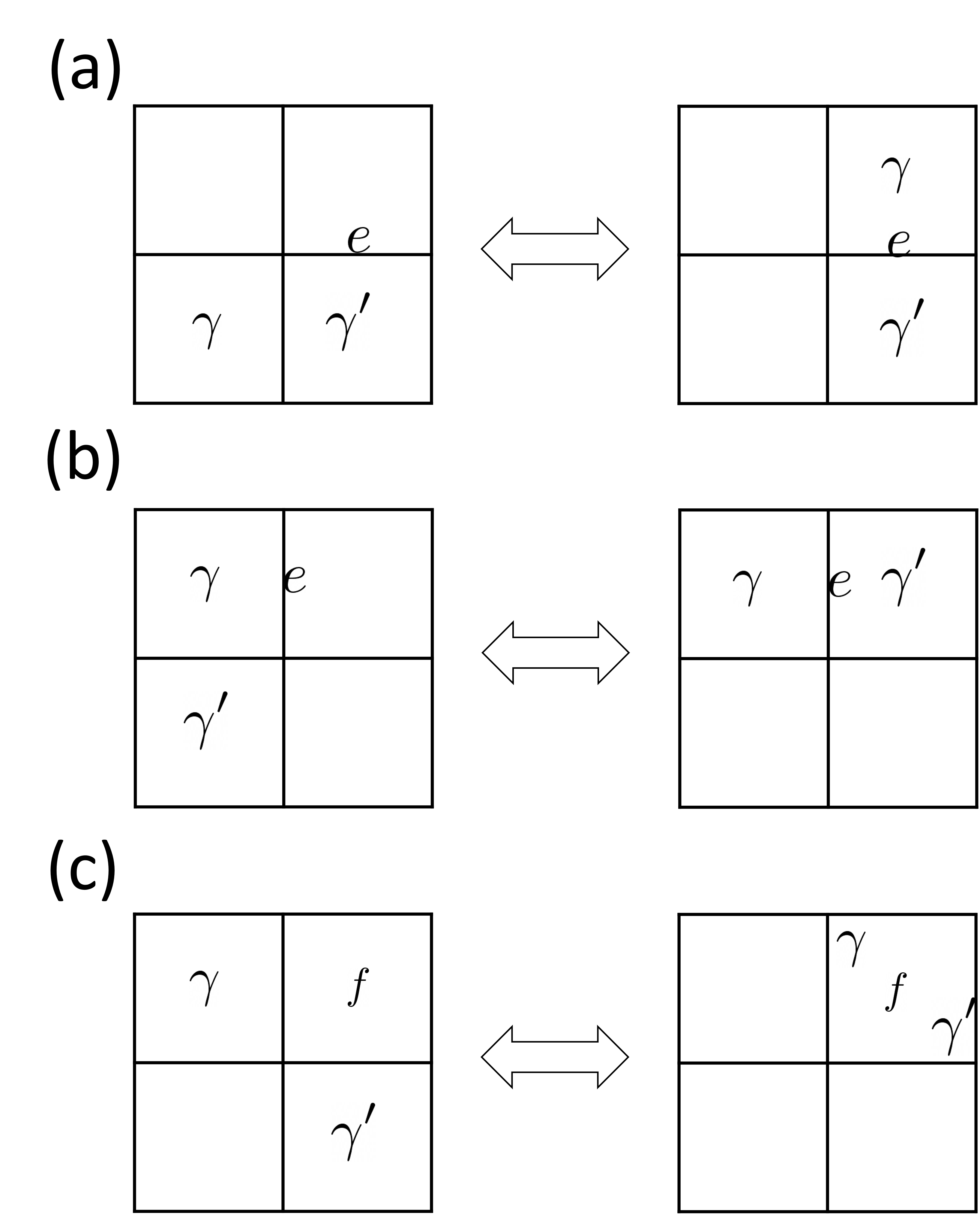
The logical operators and stabilizer in Eq. (88) is exactly the logical operators and stabilizers of exact bosonization after a shift of Majorana fermions. If we shift the Majorana fermions in the exact bosonization as Fig. 17 and re-pair them. Then we find the exact bosonization and the Verstraete-Cirac mapping are equivalent, as Fig. 18.
IV.3 Kitaev’s honeycomb model
The Hamiltonian of Kitaev’s honeycomb model Kitaev 2006 can be written as
| (89) |
where , , links are shown in Fig. 19. The qubit at each site can be represented by four Majorana operators , , and with an additional constraint to eliminate the redundancy at each site . The Pauli matrices at each site can be represented as follows:
| (90) |
or equivalently (after multiplying by )
| (91) |
Then, a free-fermion Hamiltonian
| (92) |
is equivalent to a sector of Eq. (89), where the index takes values , or depending on the direction of the link . Focusing on the algebra generated by , the mapping Eq. (90) can be written as Chen et al. 2018:
| (93) |
and the product of Majorana hoppings along a hexagon is proportional to identity, which gives a gauge constraint on the qubit Hilbert space. It is shown Chen et al. 2018 that by embedding the honeycomb lattice into the square lattice as Fig. 20, relabeling by , and performing single-qubit rotations, the complete bosonization map can be expressed as
with gauge constraints
| (122) |
This is equivalent to the logical operators and stabilizers in Eq. (88) up to a shift. Therefore, it is gLU equivalent to the exact bosonization.


IV.4 Majorana loop stabilizer codes

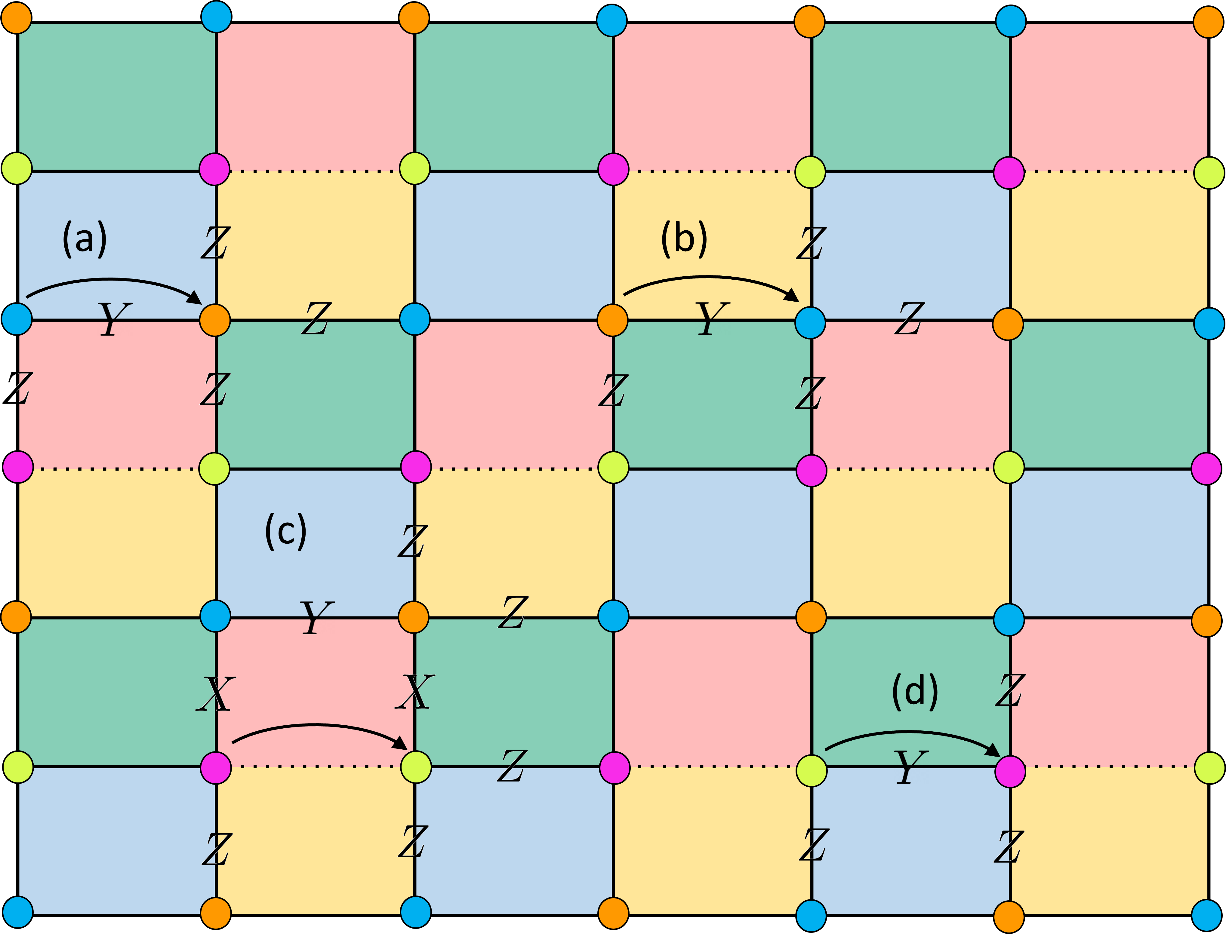
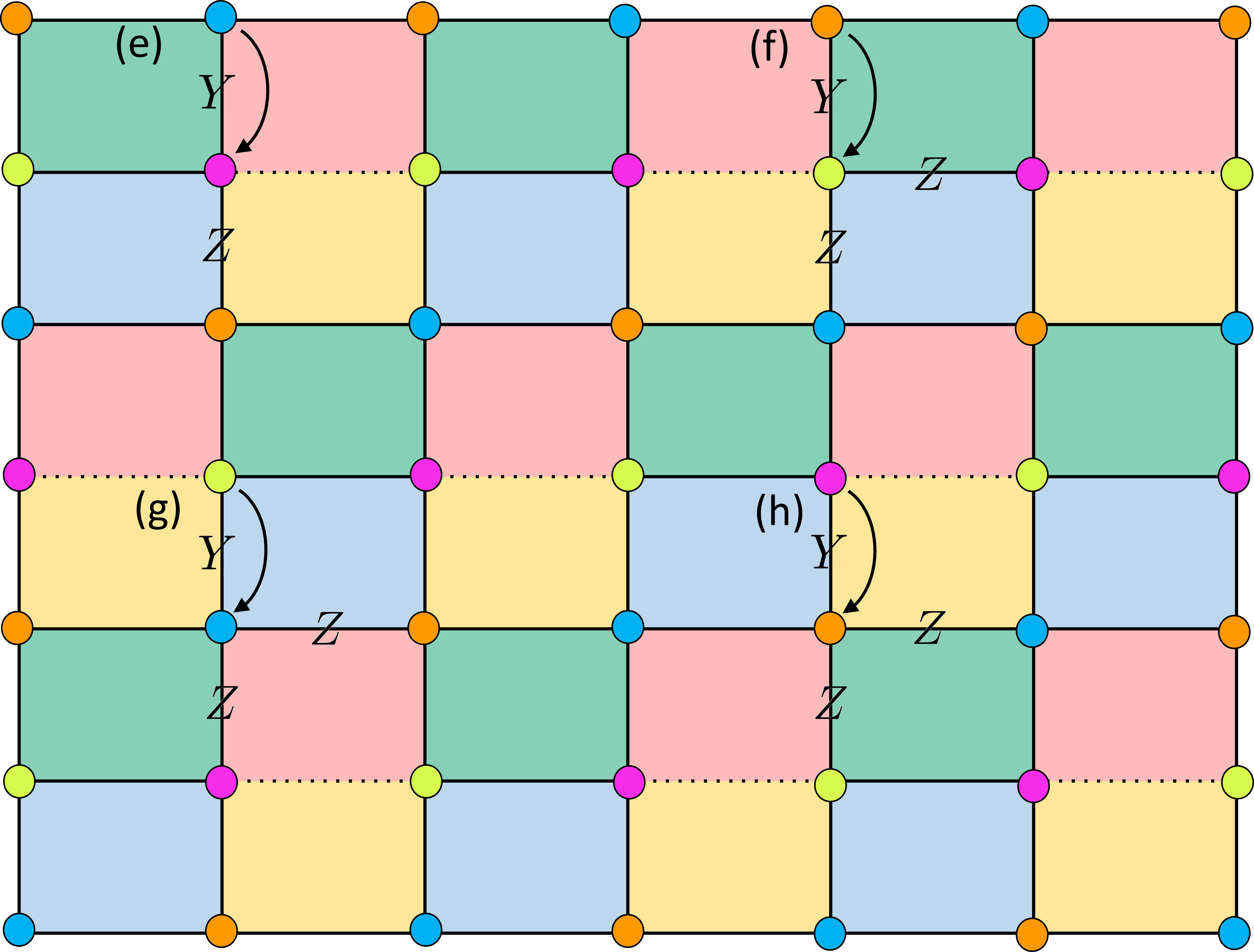
In this section, we show that Majorana loop stabilizer code (MLSC) Jiang et al. 2019 is gLU equivalent to the 2d exact bosonization. Similar to BKSF, the Majorana loop stabilizer codes encode a complex fermion on vertex by qubits on edge connected to . The Majorana loop stabilizer codes have fermionic hopping operation on each edge, fermion parity operator on each vertex and stabilizers acting on faces with different colors. We follow the same procedure described in Sec. III, conjugating the logical operations and stabilizers of MLSC by finite-depth Clifford circuits in Fig. 21. Then the four kinds of horizontal hoppings in MLSC reduce to the horizontal hopping in the exact bosonization (up to a stabilizer), and the same thing happens to the vertical hoppings, parity operators, and stabilizers.
Starting from the MLSC, Fig. 22 and Fig. 23 shows that the horizontal and vertical hoppings after the transformation can match the horizontal and vertical hoppings in exact bosonization. An interesting fact is that the first Clifford circuit in Fig. 21 removes qubit on the edges between red and yellow squares and makes this correspondence possible.
IV.5 Connection to Jordan-Wigner transformation
In this section, we will show that conjugating the exact bosonization by a linear-depth1212 12 The depth of the circuit scales linearly with the system size. Clifford circuit in Fig. 24 will result in the 1d Jordan-Wigner transformation along the path in Fig. 25.
For the Jordan-Wigner transformation, the qubit-fermion ratio is 1, but it is a non-local fermion-to-qubit mapping since in 1d Jordan-Wigner transformation, the vertical hopping terms are mediated by a Pauli -string between two sites. By directly applying the linear-depth gLU Clifford circuit in Fig. 24 to the logical operators of the exact bosonization, the qubits on the horizontal edges are disentangled and do not show up in the logical operators. All stabilizers become single-Pauli operators on horizontal edges and can be removed by gLU transformations. Explicitly, the logical operators after conjugation of the Clifford circuit are:

which is exactly the 1d Jordan-Wigner transformation with the ordering chosen in Fig. 25. Hence, we can regard 1d Jordan-Wigner transformation as a special case that we remove all the qubits on the horizontal edges where the vertical hoppings are no longer local.

Acknowledgement
Y.-A.C thanks Mark Steudtner for pointing out the equivalence between the BKSF and the exact bosonization. Y.-A.C want to thank Anton Kapustin, Tyler Ellison and Nat Tantivasadakarn for useful discussions. Y.-A.C is also thankful to Bowen Yang for teaching the classification of Pauli stabilizer models in two dimensions. Y.-A.C is supported by the JQI fellowship at the University of Maryland. Y.X. is supported by ARO W911NF-15-1-0397 and advisor Mohammad Hafezi.
Appendix A Clifford gates
The Clifford group is defined as the group of unitaries that normalize the Pauli group. The Clifford gates are defined as elements in the Clifford group Gottesman 1998a; Gottesman 1998b. In this paper, we use single-qubit Clifford gates: -gate, -gate, -gate.
The -gate is the Hadamard gate
| (150) |
that satisfies , .
The -gate is the phase gate
| (151) |
that satisfies , .
The -gate is
| (152) |
where , .
For 2-qubit Clifford gates, we choose , and gate. The gate is
| (153) |
where
| (154) |
The (controlled-) gate is
| (155) |
where
| (156) |
The (controlled-) gate is
| (157) |
where
| (158) |
References
- Chen et al. (2018) Yu-An Chen, Anton Kapustin, and Djordje Radicevic, “Exact bosonization in two spatial dimensions and a new class of lattice gauge theories,” Annals of Physics 393, 234 – 253 (2018).
- Verstraete and Cirac (2005) F Verstraete and J I Cirac, “Mapping local hamiltonians of fermions to local hamiltonians of spins,” Journal of Statistical Mechanics: Theory and Experiment 2005, P09012–P09012 (2005).
- Kitaev (2006) Alexei Kitaev, “Anyons in an exactly solved model and beyond,” Annals of Physics 321, 2–111 (2006).
- Whitfield et al. (2016) James D. Whitfield, Vojt ěch Havlíček, and Matthias Troyer, “Local spin operators for fermion simulations,” Phys. Rev. A 94, 030301 (2016).
- Jiang et al. (2019) Zhang Jiang, Jarrod McClean, Ryan Babbush, and Hartmut Neven, “Majorana loop stabilizer codes for error mitigation in fermionic quantum simulations,” Physical Review Applied 12 (2019), 10.1103/physrevapplied.12.064041.
- Setia et al. (2019) Kanav Setia, Sergey Bravyi, Antonio Mezzacapo, and James D. Whitfield, “Superfast encodings for fermionic quantum simulation,” Phys. Rev. Research 1, 033033 (2019).
- Bochniak and Ruba (2020) A. Bochniak and B. Ruba, “Bosonization based on clifford algebras and its gauge theoretic interpretation,” Journal of High Energy Physics 2020, 118 (2020).
- Derby et al. (2021) Charles Derby, Joel Klassen, Johannes Bausch, and Toby Cubitt, “Compact fermion to qubit mappings,” Phys. Rev. B 104, 035118 (2021).
- Po (2021) Hoi Chun Po, “Symmetric jordan-wigner transformation in higher dimensions,” arXiv preprint arXiv:2107.10842 (2021).
- Bravyi and Kitaev (2002) Sergey B Bravyi and Alexei Yu Kitaev, “Fermionic quantum computation,” Annals of Physics 298, 210–226 (2002).
- Chen and Kapustin (2019) Yu-An Chen and Anton Kapustin, “Bosonization in three spatial dimensions and a 2-form gauge theory,” Phys. Rev. B 100, 245127 (2019).
- Chen (2020) Yu-An Chen, “Exact bosonization in arbitrary dimensions,” Phys. Rev. Research 2, 033527 (2020).
- Ellison and Fidkowski (2019) Tyler D. Ellison and Lukasz Fidkowski, “Disentangling interacting symmetry-protected phases of fermions in two dimensions,” Phys. Rev. X 9, 011016 (2019).
- Chen et al. (2021) Yu-An Chen, Tyler D. Ellison, and Nathanan Tantivasadakarn, “Disentangling supercohomology symmetry-protected topological phases in three spatial dimensions,” Phys. Rev. Research 3, 013056 (2021).
- Chen and Hsin (2021) Yu-An Chen and Po-Shen Hsin, “Exactly solvable lattice hamiltonians and gravitational anomalies,” arXiv preprint arXiv:2110.14644 (2021).
- Bravyi et al. (2010) Sergey Bravyi, Barbara M Terhal, and Bernhard Leemhuis, “Majorana fermion codes,” New Journal of Physics 12, 083039 (2010).
- Vijay and Fu (2016) Sagar Vijay and Liang Fu, “Physical implementation of a majorana fermion surface code for fault-tolerant quantum computation,” Physica Scripta 2016, 014002 (2016).
- Viyuela et al. (2019) Oscar Viyuela, Sagar Vijay, and Liang Fu, “Scalable fermionic error correction in majorana surface codes,” Phys. Rev. B 99, 205114 (2019).
- Vijay et al. (2015) Sagar Vijay, Timothy H. Hsieh, and Liang Fu, “Majorana fermion surface code for universal quantum computation,” Phys. Rev. X 5, 041038 (2015).
- Litinski and von Oppen (2018) Daniel Litinski and Felix von Oppen, “Quantum computing with majorana fermion codes,” Phys. Rev. B 97, 205404 (2018).
- Hastings (2017) M. B. Hastings, “Small majorana fermion codes,” (2017), arXiv:1703.00612 [quant-ph] .
- Gottesman (1998a) Daniel Gottesman, “Theory of fault-tolerant quantum computation,” Phys. Rev. A 57, 127–137 (1998a).
- Gottesman (1998b) Daniel Gottesman, “The heisenberg representation of quantum computers,” arXiv preprint quant-ph/9807006 (1998b).
- Chen et al. (2010) Xie Chen, Zheng-Cheng Gu, and Xiao-Gang Wen, “Local unitary transformation, long-range quantum entanglement, wave function renormalization, and topological order,” Phys. Rev. B 82, 155138 (2010).
- Zeng et al. (2018) Bei Zeng, Xie Chen, Duan-Lu Zhou, and Xiao-Gang Wen, “Quantum information meets quantum matter – from quantum entanglement to topological phase in many-body systems,” (2018), arXiv:1508.02595 [cond-mat.str-el] .
- Freedman and Hastings (2020) Michael Freedman and Matthew B. Hastings, “Classification of quantum cellular automata,” Communications in Mathematical Physics 376, 1171–1222 (2020).
- Haah (2021a) Jeongwan Haah, “Clifford quantum cellular automata: Trivial group in 2d and witt group in 3d,” Journal of Mathematical Physics 62, 092202 (2021a), https://doi.org/10.1063/5.0022185 .
- Tarantino and Fidkowski (2016a) Nicolas Tarantino and Lukasz Fidkowski, “Discrete spin structures and commuting projector models for two-dimensional fermionic symmetry-protected topological phases,” Phys. Rev. B 94, 115115 (2016a).
- Tarantino and Fidkowski (2016b) Nicolas Tarantino and Lukasz Fidkowski, “Discrete spin structures and commuting projector models for two-dimensional fermionic symmetry-protected topological phases,” Phys. Rev. B 94, 115115 (2016b).
- Haah et al. (2018) Jeongwan Haah, Lukasz Fidkowski, and Matthew B Hastings, “Nontrivial quantum cellular automata in higher dimensions,” arXiv preprint arXiv:1812.01625 (2018).
- Haah (2021b) Jeongwan Haah, “Classification of translation invariant topological pauli stabilizer codes for prime dimensional qudits on two-dimensional lattices,” Journal of Mathematical Physics 62, 012201 (2021b), https://doi.org/10.1063/5.0021068 .