Spatiotemporal Clustering with Neyman-Scott Processes via Connections to Bayesian Nonparametric Mixture Models
Abstract
Neyman-Scott processes (NSPs) are point process models that generate clusters of points in time or space. They are natural models for a wide range of phenomena, ranging from neural spike trains to document streams. The clustering property is achieved via a doubly stochastic formulation: first, a set of latent events is drawn from a Poisson process; then, each latent event generates a set of observed data points according to another Poisson process. This construction is similar to Bayesian nonparametric mixture models like the Dirichlet process mixture model (DPMM) in that the number of latent events (i.e. clusters) is a random variable, but the point process formulation makes the NSP especially well suited to modeling spatiotemporal data. While many specialized algorithms have been developed for DPMMs, comparatively fewer works have focused on inference in NSPs. Here, we present novel connections between NSPs and DPMMs, with the key link being a third class of Bayesian mixture models called mixture of finite mixture models (MFMMs). Leveraging this connection, we adapt the standard collapsed Gibbs sampling algorithm for DPMMs to enable scalable Bayesian inference on NSP models. We demonstrate the potential of Neyman-Scott processes on a variety of applications including sequence detection in neural spike trains and event detection in document streams.
1 Department of Statistics, University of Michigan, Ann Arbor, MI, USA
2 Department of Electrical Engineering, Stanford University, Stanford, CA, USA
3 Center for Neural Science, New York University, New York, NY, USA
4 Center for Computational Neuroscience, Flatiron Institute, New York, NY, USA
5 Department of Statistics and Wu Tsai Neurosciences Institute, Stanford University, Stanford, CA, USA
∗ Equal Contribution
† Corresponding Author: scott.linderman@stanford.edu
Keywords: Neyman-Scott process, mixture of finite mixture model, Dirichlet process, collapsed Gibbs
1 Introduction
Many natural systems give rise to discrete sets of events in time and space. Biological neurons communicate with one another via sequences of spikes. Social network users share time-stamped messages with text, images, and other metadata. A fundamental challenge is to develop statistical models and inference algorithms that can provide insight into such systems and enable accurate predictions of future events.
Poisson processes are clearly suited to this task [1]. However, real systems may not obey the strict independence assumptions these models impose. In a Poisson process, the number of events in one interval of time is independent of the number of events in nearby but non-overlapping intervals. This assumption is often violated in practice.
Consider a simple model of a bursty neuron [2]. Suppose the neuron typically fires action potentials (spikes) at a low rate of spikes/second, and in this regime it may be well modeled as a homogenous Poisson process. However, suppose that every so often the neuron emits bursts of around action potentials in the span of a few hundred milliseconds. If 3 spikes are measured in a 100ms window of time, it is likely that the neuron is in the middle of a burst so we would expect to see more spikes in the following 100ms as well.
While these dependencies across disjoint intervals defy the basic assumptions of a Poisson process, the neural spike times may still be well modeled as conditionally Poisson. For example, suppose we know there are bursts that occur at times . Then the spike times might be modeled as an inhomogeneous Poisson process with conditional intensity [3],
where denotes the Gaussian density function with mean and variance . According to this model, weighted Gaussian impulse responses are superimposed on top of the constant background rate to produce bursts of spikes, clustered together in time.
Neyman-Scott processes (NSPs) [4] are point processes that capture this clustering property. In an NSP, the cluster centers (the burst times in our example) are treated as latent variables. Conditioned on these latent variables, the observed events follow an inhomogeneous Poisson process. Marginalizing over the latent variables induces dependencies across intervals that could not be captured with a simple Poisson process.
The Neyman-Scott process follows a simple generative model. First, a set of latent events is drawn from a Poisson process. Then, each latent event adds an impulse response to the intensity function of another Poisson process, which produces the set of observed events. If the impulse responses are localized in time and space, then each latent event produces a cluster of observed events. The Neyman-Scott process is a type of doubly stochastic point process (a.k.a. Cox process) since the intensity itself is a stochastic process.
The set of underlying latent events is often of scientific interest. For example, we may want to relate a neuron’s burst times to a sensory stimulus or behavioral covariate. However, this can be challenging from a statistical perspective, since neither the number of latent events nor their locations are known. Traditionally, inference and estimation in NSPs has been approached with reversible jump Markov chain Monte Carlo (RJMCMC) algorithms [5], which use birth and death moves to address this trans-dimensional inference problem [6]. However, in practice, RJMCMC can suffer from high rejection rates, sacrificing performance unless proposals are carefully crafted. Alternatively, there are a number of specialized algorithms based on minimum contrast estimation, which optimize the parameters of the NSP to match statistics of the data, such as Ripley’s K-function [7] or the pair correlation function [8, 9, 10, 11, 12, 13]. However, obtaining closed-form expressions for these second-order statistics often requires strong assumptions about the parametric form of the NSP [14, 15].
Here, we establish a novel connection between NSPs and Bayesian nonparametric mixture models, and in doing so we inherit the host of Bayesian inference algorithms that have been developed for the latter [16, 17, 18, 19]. Intuitively, latent events are akin to clusters in a mixture model. The key observation is that in an NSP, the number of latent events is a Poisson random variable. In this regard, the NSP differs from the Dirichlet process mixture model (DPMM) [20, 21, 22, 23] — the canonical Bayesian nonparametric mixture model — since a DPMM produces a countably infinite number of clusters. Instead, the NSP more closely resembles the mixture of finite mixture model (MFMM), which assumes an explicit prior distribution on the number of clusters [24, 25, 26, 27]. In an NSP, that prior is a Poisson distribution and, in contrast to other MFMMs, its mean is tuned to the volume of space or time under consideration, making the NSP especially well-suited to spatiotemporal modeling.
In this paper, we will formalize the connection between Neyman-Scott processes and mixture of finite mixture models. Furthermore, we show how Dirichlet process mixture models arise as a limiting form of an NSP, and in doing so we bridge MFMMs and DPMMs. We exploit the novel connection to derive a collapsed Gibbs sampling algorithm like that of Neal 2000 and Miller and Harrison 2018, which operates directly on partitions of data points. Finally, we demonstrate the efficacy of this algorithm on simulated data and in applications to sequence detection in multineuronal spike train recordings and event detection in document streams.
2 Neyman-Scott Processes
Point processes are probabilistic models that yield random finite sets of points , where is a compact subset of , e.g. of space or time [3]. The simplest point process is the Poisson process [1], which is governed by a nonnegative intensity function . The number of events that fall in a region follows a Poisson distribution with mean . Moreover, the number of events in is independent of the number in if and are disjoint. We use the notation to indicate that a set is drawn from a Poisson process with intensity function . A marked Poisson process is a Poisson process that generates sets of tuples with locations and marks according to an intensity function .
Neyman-Scott processes [4] are doubly stochastic processes (also known as Cox processes [28]) in which the intensity is derived from a Poisson process. First, a set of latent events is drawn from a marked Poisson process,
| (1) |
Each latent event includes a location , a non-negative weight , and, optionally, extra parameters, . Without loss of generality, assume , where is a normalized probability density and is the total measure. Thus, the number of latent events is a Poisson random variable, .
Then, each latent event adds a non-negative impulse response to the intensity of another marked Poisson process, which produces the observed data points,
| (2) | ||||
| (3) |
As above, we assume is a probability density which is scaled up or down by the weight, . Dependencies between the weights, locations, and parameters can be incorporated into the latent event intensity function .
2.1 Example applications of Neyman-Scott processes
Neyman-Scott processes are applicable to a wide variety of spatiotemporal clustering problems. Figure 1 highlights three examples, which we will return to in our experiments.
Modeling the locations of trees in a forest
Consider modeling the locations of trees in a forest. Trees of the same species may cluster together if they grow from seeds dropped by a shared ancestor. Neyman-Scott processes have been used to model this type of spatial point process data [29, 30]. Let denote a compact subset of the 2-dimensional plane, like the square shown in Figure 1 (left). Likewise, let , , and denote the location, covariance, and weight of a cluster of trees, respectively, and assume the impulse responses are scaled Gaussian densities, . In Figure 1 (left), we set the latent event intensity to be homogenous in space and proportional to a gamma density and inverse Wishart density in the weight and covariance, respectively.
Finding sequences of spikes in neural recordings
With multielectrode arrays, neuroscientists can record the times at which individual neurons fire action potentials, or spikes. A sequence of spike times from one or more neurons is called a spike train. We can model a spike train as a collection of tuples where denotes the time of the -th spike and denotes the index of the neuron on which it occurred. An important problem in neuroscience is detecting sequences of spikes that unfold across multiple neurons and recur many times over the course of a recording [31, 32]. This is an extension of the burst-detection problem in Section 1.
Consider the following Neyman-Scott process model for sequence detection, as described by Williams et al. 2020. Each sequence corresponds to a latent event, which consists of a time (i.e. location) , weight , and a discrete type (i.e. parameter) . The hyperparameter specifies the number of sequence types, and each neuron may spike with different probability and delay under different sequence types. By varying the offsets, a single latent event can induce a sequence of spikes across a set of neurons, and different sequence types can engage different subsets of neurons, as shown in Figure 1 (middle).
Detecting world events from streams of news documents
Finally, suppose we have a collection of documents, each with a timestamp, author, and a string of words. For example, they may be diplomatic cables exchanged between multiple countries. We represent the dataset as where denotes the time stamp. The mark is another tuple , where denotes the index of the document’s author and denotes a vector of word counts for each term in a vocabulary of size . Compared to previous examples, these are very high dimensional marks.
The idea is that documents that discuss the same event were likely written around the same time and use similar terms. For example, we might see a flurry of diplomatic cables following an election. In many cases, those events are latent and we aim to infer them from the observed documents. To perform event detection with a Neyman-Scott process, let the latent events of the NSP consist of a time , weight , and parameters . The first parameter is a distribution over authors; the second is a vector of intensities for each word in the vocabulary, as illustrated in Figure 1 (right).
2.2 Simulating a Neyman-Scott process
These examples bear strong resemblance to mixture models, with each latent event corresponding to a cluster. The Poisson superposition principle [1] makes this connection explicit. Given the set of latent events, the intensity function in eq. 2 is a sum of non-negative impulse responses. To simulate such a Poisson process, we can independently sample data points from Poisson processes for each impulse response and take their union.
To sample data points for each impulse response, first sample the number of induced data points, then sample their locations and marks independently according to the normalized impulse response. Since the impulse responses are weighted probability density functions, the expected number of induced data points is simply the weight, , and the normalized impulse responses are simply the conditional densities, . This procedure for sampling an NSP is shown in Algorithm 1.
This sampling procedure lets us interpret the Neyman-Scott process as a clustering model in which each data-point is attributed to of one of the underlying latent events. Moreover, under the NSP, the number of clusters is a random variable, suggesting a connection between Neyman-Scott processes and Bayesian nonparametric mixture models. We formalize this relationship in the next section.
3 Neyman-Scott Processes and Bayesian Nonparametric Mixture Models
Our first contribution is to establish a connection between Neyman-Scott processes, Dirichlet process mixture models (DPMMs) [20, 21, 22, 23], and the mixture of finite mixture model (MFMM) recently studied by Miller and Harrison 2018. MFMMs are Bayesian mixture models in which the number of clusters is a finite random variable. We will show how the NSP can be seen as an MFMM in which the distribution of the number of components depends on how many data points are observed. This relationship allows us to extend many of the results of Miller and Harrison 2018 and characterize the NSP in terms of its random partition distribution, urn scheme, and random measure formulation. In doing so, we will see that the Neyman-Scott Process occupies a privileged place among MFMMs: in a certain limit, the NSP reduces to the classic DPMM. This relationship allows the Neyman-Scott process to interpolate between these two important model classes and inherit the efficient inference algorithms available for DPMMs and MFMMs.
To establish the connection to MFMMs and DPMMs, we first present an equivalent sampling procedure for Neyman-Scott processes. Rather than sampling the numbers of induced data points, , for each of the latent events, we first sample the total number of induced data points, , and then assign each data point a parent latent event. Since each is an independent Poisson random variable, the total number of induced data points is also Poisson distributed and the parents are categorical random variables [1]. The alternative algorithm is shown in Algorithm 2.
The sampling procedure simplifies even further under the following assumption.
Assumption 1.
The latent event intensity factors as,
| (4) |
That is, the latent event weights are gamma random variables with shape and inverse scale , and they are independent of the latent event locations and parameters.
Under this assumption, the Neyman-Scott process becomes a shot noise G Cox process [34, 6], which is closely related to the Poisson-gamma process [35], multiplicative intensity models [36], and Lévy-moving averages [37]. We will simply call it an NSP with gamma weights.
The total weight in Algorithm 2 is the sum of independent and identically distributed gamma random variables, which is also a gamma distributed, . Moreover, the normalized weights in Algorithm 2 follow a symmetric Dirichlet distribution, , where is a length- vector of ones. Under the gamma distribution, the total weight is independent of the normalized weights [38]. Algorithm 3 uses these three properties to sample an NSP with gamma weights, per Assumption 1 above. Finally, since the gamma and Poisson are conjugate, we can marginalize over the total weight to obtain a negative binomial distribution on the number of data points, as in collapsed sampling procedure in Algorithm 4.
Compare Algorithm 4 to Algorithm 5 for sampling an MFMM, adapted from Miller and Harrison 2018. There are three main differences. First, the MFMM allows for arbitrary distributions on the number of components, , a p.m.f. on the positive integers, whereas the NSP has a Poisson distribution. Second, the number of latent events in an NSP depends on the total measure over the domain ; that is, an NSP can generalize from one domain to another and scale the expected number of latent events accordingly. Third, the MFMM treats the number of observed events as fixed, whereas the NSP model treats as a random variable that depends on the number of latent events, .
Conditioned on the number of data points, however, the Neyman-Scott process with gamma weights is a special case of the mixture of finite mixtures model. In an NSP, the number of data points carries information about the number of latent events—intuitively, more data points suggests more clusters. In particular, given that we have observed data points, the NSP with gamma weights is a special case of the MFMM in which , where is the negative binomial probability mass function (pmf). This distribution is closely related to a shifted confluent hypergeometric distribution, which we call the Schein distribution after Schein et al. 2019. The Schein distribution is in turn closely related to the Pólya-Aeppli distribution [40]. Its pmf has a closed-form expression in terms of hypergeometric functions.
The correspondence between NSPs and MFMMs enables many of the results of Miller and Harrison 2018 to be adapted to the Neyman-Scott process. In particular, we will derive the marginal distribution over partitions of data points in an NSP and a corresponding Pólya urn scheme, which leads to yet another algorithm for sampling Neyman-Scott processes. This urn scheme will suggest an efficient collapsed Gibbs sampling algorithm for posterior inference in NSPs with gamma weights, which we develop in Section 5. Moreover, the urn scheme reveal a novel connection between Neyman-Scott processes and Dirichlet process mixture models.
3.1 The exchangeable partition distribution of a Neyman-Scott process
The Neyman-Scott process induces a random partition of data points into clusters associated with different latent events. Let denote the number of observed data points and denote a partition of the indices induced by the parent assignments in Algorithm 4. In other words, is a set of disjoint, non-empty sets whose union is . We represent the partition as , where is the set of data indices assigned to latent event and is the size of that cluster. The size of the partition, , is the number of latent events that induced at least one observed data point, so we must have .
The parent assignments induce a partition of the observed events, but they are tied to a particular labeling of the latent events. The partition, by contrast, is invariant to permutations of the latent event indices. Working with partitions frees us from keeping track of latent event indices or empty components in mixture models—we only need to infer how the finite number of data points are partitioned into different components.
Theorem 1.
Under Assumption 1, the prior probability of the partition induced by an NSP, integrating over the latent event locations, weights, and parameters, is,
| (5) |
where and are the shape and rate, respectively, of the gamma prior on latent event weights, is the number of clusters in the partition, is the size of the -th cluster in the partition, is the total number of data points (a random variable), and
| (6) |
Theorem 1 and its proof (given in Appendix A) closely parallel the main theorem of Miller and Harrison 2018, which gives the partition distribution for mixture of finite mixture models. The main difference is that eq. 5 is a distribution on partitions of random size . To obtain a conditional distribution on partitions of given size —the partition distribution more commonly considered [41, 24]—we need to divide by the probability of obtaining data points,
| (7) |
The distribution above is a Poisson-mixed negative binomial. It does not, to our knowledge, have an analytical form, but we will not need one for our purposes.
Note that is a symmetric function of the cluster sizes, , and therefore it is invariant to permutations of the integers . Thus, is an exchangeable random partition and is an exchangeable partition probability function (EPPF) [41]. In particular, it takes the form of a Gibbs partition [42] since it factors into a term that depends on the number of data points and clusters () and a product of rising factorials () depending on the size of each cluster.
The EPPF offers yet another way of sampling a Neyman-Scott process as shown in Algorithm 6. First sample a random partition , which specifies the number of data points; then sample parameters for each cluster in the partition; and finally, independently sample data points for each cluster. The key step is sampling a random partition, and as we will see in the next section, this can be done with a simple Pólya-urn process. The main advantage of this formulation is that it only involves the partition, cluster parameters, and data points, and that enables the simple collapsed Gibbs sampling algorithm for NSPs presented in Section 5.
b. new cluster w/pr end for
3.2 Connecting Neyman-Scott processes and Dirichlet process mixture models
Like the MFMM and other nonparametric mixture models, the Neyman-Scott process can be characterized by its Pólya-urn scheme (aka “restaurant process”). A Pólya-urn scheme is a discrete-time Markov process on partitions of the integers. Indices are introduced one at a time, and they are either added to an existing cluster or to a new, singleton cluster. The Blackwell-MacQueen urn scheme [43] (aka “Chinese restaurant process”) and Pitman-Yor process [44] are classic examples. We will show that the Neyman-Scott process corresponds to an urn scheme of a very similar nature, and, like the two-parameter Pitman-Yor process, it subsumes the Blackwell-MacQueen urn scheme as a limiting case.
The following corollary describes an urn scheme in which the marginal distribution after steps is .
Theorem 2.
Let be a partition of the integers . The following transition operator is a distribution on partitions of the integers that equal when the integer is removed.
| (8) |
Starting with and applying this transition operator times yields a partition of the integers that is distributed according to .
Theorem 2 is equivalent to Theorem 4.1 of Miller and Harrison 2018 for mixture of finite mixture models, which is unsurprising since we have already shown that Neyman-Scott processes are special cases of MFMMs when conditioned on the number of data points.
Here is where the Neyman-Scott process distinguishes itself from other mixture of finite mixture models. In the NSP, the ratio is a constant determined only by the latent event intensity and the parameters of the weight distribution.
Lemma 1.
Under a Neyman-Scott process satisfying Assumption 1,
| (9) |
The proof of this lemma follows from simple substitution, as shown in Appendix A. This ratio controls the probability of adding a new cluster in the urn process described in Theorem 2. In general MFMMs, the ratio changes as a function of and , and Miller and Harrison 2018 recommend precomputing it for a range of values. For Neyman-Scott processes with gamma weights, it is simply a constant.
Lemma 1 also hints at a close relationship between NSPs and Dirichlet process mixture models. Recall that in the Blackwell-MacQueen urn scheme that generates partitions of Dirichlet process mixture model, the probability of adding a new cluster is also constant [43]. Specifically, the probability of adding to an existing cluster is proportional to the size of the cluster, , and the probability of creating a new cluster is proportional to a constant , the Dirichlet process concentration. The following corollary formalizes this relationship, showing how the DPMM arises when as a limiting case of the NSP with infinitely many latent events with weights that are almost surely zero.
Corollary 3.
The Neyman-Scott process with gamma weights (Assumption 1) approaches a Dirichlet process mixture model with concentration and a base measure with density in the limit that while .
Proof.
In this limit, the probability of adding a new cluster is and the probability of adding to an existing cluster is . Thus, the urn scheme given in Theorem 2 converges to the Blackwell-MacQueen urn scheme, which underlies the Dirichlet process mixture model. The cluster parameters in the NSP are sampled i.i.d. from in the same way cluster parameters are sampled independently from the base measure in a DPMM. ∎
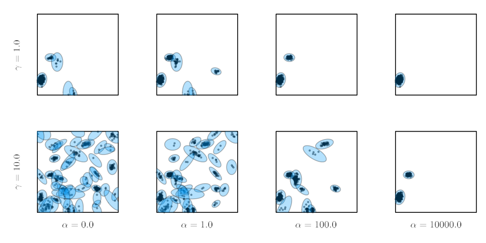
Figure 2 shows realizations of the NSP urn scheme for data points. In each row, the shape parameter is varied while the inverse scale is fixed and the latent event rate is changed so that is held constant. In the limit where (i.e. in the left-most column), the urn process is identical to the Blackwell-MacQueen urn process for Dirichlet process mixture models, as stated in Corollary 3. As the shape parameter is increased, there is a greater tendency to add data points to existing clusters, leading to fewer clusters for a fixed dataset size. The DPMM limit, in contrast, has a larger number of small clusters.
The Neyman-Scott urn scheme in Theorem 2 is even more similar to the urn scheme of the two-parameter Pitman-Yor process [44]. The Pitman-Yor scheme adds indices to existing clusters with probability proportional to and to a new cluster with probability proportional to . When the discount parameter is zero, the Pitman-Yor process is also equivalent to the Dirichlet process (and its urn scheme is equivalent to the Blackwell-MacQueen urn scheme). When the discount parameter is negative, the Pitman-Yor urn scheme preferentially adds to existing clusters, just like in the NSP urn scheme, suggesting a correspondence between the shape parameter in the NSP and in the Pitman-Yor scheme. However, when , the strength parameter must equal for integer so that the probability of creating a new cluster equals exactly zero once . In this case the Pitman-Yor process generates a partition for a finite Dirichlet-multinomial model. That is where the Neyman-Scott and Pitman-Yor urn schemes differ: in the NSP, the probability of creating a new cluster is proportional to a constant, regardless of the number of existing clusters; in the Pitman-Yor urn scheme with a negative discount factor, that probability decreases as the number of clusters increases. Both the Neyman-Scott and Pitman-Yor urn schemes converge to the Blackwell-MacQueen urn scheme under certain limits, but they differ in their approach.
The connection between Neyman-Scott processes and Dirichlet process mixture models is also evident from their random measures. We can view the latent events of the NSP as a discrete random measure on with a Poisson-distributed number of atoms. The -th atom is located at and has weight . Intuitively, in the limit described in Corollary 3, the number of atoms goes to infinity and the weights go to zero. In this limit, the random measure approaches a gamma process that, once normalized, yields a Dirichlet process. The induced intensity arises by convolving this random measure with an impulse response to obtain the intensity . Normalizing the intensity yields the mixture density of a DPMM. We formalize this random measure perspective in Appendix B.
4 Accounting for Background Data Points
Often, the observed data points naturally separate into those induced by latent events and those that are “background noise.” One way to account for such background events is by adding an extra term to the intensity function that produces the observed data points,
| (10) |
where is a non-negative intensity function. Then, the Neyman-Scott process sampling procedure (Algorithm 1) has one extra step of sampling background data points . The complete set of data points, , is the union of the background data points and those induced by latent events.
There are a few ways of modeling the background intensity. Without loss of generality, factor the intensity as , where is a normalized probability density on . We will primarily focus on the spatiotemporal intensity and assume the mark density is easy to model. The simplest background model is a constant, homogeneous intensity, . Under this model, the induced data points are superimposed on top of a background of uniformly distributed data points, and the number of background data points is determined by . Alternatively, could be modeled with a general, nonparametric model like a log Gaussian Cox process [45] or sigmoidal Gaussian Cox process [46]. With such models, we can incorporate any spatiotemporal covariates into the prior distribution on background intensities. Our only requirements are that we must be able to evaluate the background intensity at any point and the posterior distribution over background intensities given background data points be amenable to MCMC sampling. It is important to note that there is a risk of non-identifiability with general parametric background intensities. If the background intensity can subsume the impulse responses, then there is no way to distinguish between background and induced data points. A simple and often intuitive solution to this problem is to assume that the background intensity varies slowly relative to the impulse responses; i.e. to assume a separation of spatiotemporal scales.
Regardless of the background model, the Neyman-Scott process with an additive background intensity and gamma weights also admits a simple partition distribution. Let denote the subset of indices assigned to the background and be a partition of .
Theorem 4.
Under Assumption 1, the prior probability of the partition induced by an NSP with background intensity , marginalizing the latent event locations, weights, and parameters, is,
| (11) |
where and are the shape and rate, respectively, of the gamma prior on weights, is the number of clusters in the partition, is the size of the -th cluster in the partition, is the total number of data points (a random variable), and where is the integrated background intensity.
A partition of size can be generated recursively with the following urn scheme,
| (12) |
where is a partition of the integers and is a partition of obtained by adding index as described above.
Theorem 4 closely parallels Theorems 1 and 2, as does its proof (given in Appendix A). The only difference is that here we separate the background indices, , from the partition of the remaining indices, . In the terminology of Pitman 2006, eq. (11), once normalized by , is a partially exchangeable partition probability function since it is not symmetric in the cluster indices; the background cluster is treated differently.
5 Bayesian Learning and Inference for Neyman-Scott Processes
Having shown the relationship between Neyman-Scott processes with gamma weights, mixture of finite mixture models, and Dirichlet process mixture models, we can adapt standard collapsed Gibbs sampling algorithms for MFMMs [24] and DPMMs [47, 16] to NSPs. The resulting algorithm is quite different from existing inference algorithms for NSPs. Rather than proposing to add or remove latent events, as in reversible jump MCMC algorithms [6, 15], the collapsed Gibbs algorithm marginalizes over latent event locations and parameters and operates directly on the posterior over partitions. Unlike minimum contrast estimation methods, the collapsed Gibbs algorithm asymptotically generates samples from the posterior distribution and makes minimal assumptions about the latent events and their impulse responses.
repeat times to draw samples
a. the background cluster, , with probability
b. cluster , with probability
c. a new cluster with probability
end
for :
Sample locations and parameters
Sample weights
end
Sample hyperparamters of given the samples
Sample number of empty clusters . Set .
Sample homogenous latent event intensity
Sample weights for empty clusters for
Sample hyperparamters
Algorithm 8 assumes access to the marginal likelihood,
| (13) |
and the predictive likelihood
Closed-form expressions for these likelihoods are available for conjugate exponential family models. However, extensions for collapsed Gibbs sampling in nonconjugate DPMMs and MFMMs also apply here. If the marginal likelihood in eq. 13 is not available in closed form, auxiliary variable methods like Algorithm 8 of Neal 2000 may be used. Likewise, split-merge methods [17, 18] can improve the mixing time of the sampling algorithm with larger updates to the partition. Further details on the sampling steps, hyperparameter selection, initialization, and parallelization are in Appendix C.
6 Experiments
We study the collapsed Gibbs algorithms for the Neyman-Scott process model on synthetic data as well as real neural recordings and document streams. All of the code for our experiments is written in the Julia programming language and made publicly available in the Github repository redacted.jl. Across datasets, we find that the Neyman-Scott process (NSP) offers a compelling alternative to existing clustering models in tasks like sequence detection in neural spike train data and event detection in document streams.
6.1 Sampler convergence and performance
In our first experiment, we compare the mixing time and sampler efficiency of our collapsed Gibbs sampler with split-merge moves to a standard reversible jump MCMC sampler on a synthetic dataset. Overall, we find that the collapsed Gibbs sampler converges to the posterior more quickly and produces more effective samples per second than the reversible jump sampler.
We generate synthetic data from a 2D Neyman-Scott process across the unit square with gamma weights and Gaussian clusters. Specifically, we set
| (14) | ||||
| (15) |
where specifies the rate of latent events and denotes an inverse Wishart density with degrees of freedom and scale matrix . We set the background rate to zero for simplicity. Figure 4A shows a sample from this NSP.
We then fit an NSP to the generated data using the same priors. We initialize each Markov chain by sampling each of the parent assignments uniformly at random from the set (see Appendix C for further detail). The reversible jump MCMC sampler alternates between proposing latent event birth-death moves, sampling parent assignments conditioned on the latent event parameters, and sampling of the latent event parameters conditioned on parent assignments. Analogously, the collapsed Gibbs sampler alternates between sampling parent assignments and proposing split-merge moves, both marginalized over latent event parameters. The split-merge moves propose either splitting a cluster in two or merging an existing cluster, operating directly on the posterior over partitions. These updates, like the collapsed Gibbs updates, come directly from our derivation of the posterior probability over partitions (see Appendix C for further detail).
We run 3 independent chains of each sampler for 2 minutes ( samples each) and plot their performance in Figure 3. In Panels A and B, we display trace plots of joint log-likelihood and and the inferred number of non-empty clusters during inference. In Panel C, we plot the potential scale reduction factor (PSR, also known as ) of the number of non-empty clusters. Both samplers converge to PSR near 1.0, indicating that the independent chains have converged to the same posterior mode. Finally, Panel D shows the effective sample size for each sampler. The collapsed Gibbs sampler mixes significantly more rapidly than the reversible jump MCMC sampler.
6.2 Comparison with DPMM
Our second experiment compares the performance of the NSP with the Dirichlet process mixture model (DPMM) on the same synthetic dataset. Our results indicate that a DPMM cannot model data from an NSP well: it leads to inaccurate cluster assignments and a biased estimate of the number of clusters.
We use the same synthetic data and collapsed Gibbs sampler as in Section 6.1 to fit both models, running 3 independent chains per model. Figure 4, panels B and C show the resulting parent assignments at the end of sampling one of the three chains, for each the NSP and the DPMM. We observe that the inferred assignments using the NSP qualitatively outperform those of the DPMM. To quantitatively assess the accuracy of the inferred parent assignments, we use co-occupancy accuracy. Let and denote the parent assignments obtained from partitions and , assuming arbitrary ordering of their clusters. The co-occupancy accuracy is defined as, where is the binary indicator function. Panel D shows the co-occupancy accuracy of the resulting partition for the last 100 samples of each chain. Finally, Panel E shows the inferred number of clusters over the same duration. The NSP infers both co-occupancy and the number of clusters more accurately than the DPMM. These results suggest that the DPMM is not an appropriate model for fitting data generated by an NSP (or an MFMM, see [24] for additional examples).
6.3 Application: Detecting sequences in neural spike trains
We next apply the Neyman-Scott process model to perform sequence detection in neural data. With multielectrode arrays, neuroscientists can record the times at which individual neurons fire action potentials, or spikes. A collection of spike times from one or more neurons is called a spike train. In many experimental settings, groups of neurons (sometimes called “ensembles”) are hypothesized to fire repeatedly in sequences [48, e.g.]. Identifying these sequences in spike train data is a longstanding problem that has spurred a wide variety of modeling approaches [31, 32, 49, 50]. The results below extend Williams et al. 2020.
We model the spike train as a marked point process generated by the Neyman-Scott process described in Section 2. Each sequence corresponds to a latent event, which consists of a time , weight , and a discrete type . We model the latent event intensity as, , where is a distribution over sequence types. We model the conditional intensity of the observed spikes as,
| (16) |
where sets the rate of background spikes across all neurons, is a distribution over neurons, is a distribution over neurons for spikes in sequences of type , and and specify the latency and width, respectively, of impulse responses induced on neuron by latent events of type .

We applied the Neyman-Scott process to a recording of higher vocal center (HVC) premotor neurons in a zebra finch, which generate sequences that are time-locked to syllables in the bird’s courtship song. Figure 5A shows a qualitative comparison of the performance of a discrete time method called convNMF [50] and the Neyman-Scott process for neural sequence detection. The raw data (top panel) showed no visible spike patterns; however, clear sequences were revealed by sorting the neurons lexographically by preferred sequence type and the temporal offset parameter, as inferred by the Neyman-Scott process. While both models extracted similar sequences, the Neyman-Scott process provided a finer scale annotation of the final result, offering, for example, attributions at the level of individual spikes to sequences.
Further, the Neyman-Scott process offered uncertainty estimates for key parameters via the MCMC samples. Figure 5B summarizes uncertainty in the total number of latent events pooled over 10 independent MCMC runs with different random seeds—the chains differ slightly in their estimates, with medians differing by 1-2 sequences across chains. The uncertainty is largely due to the rapid sequences (in blue) shown in panel A. Figure 5C displays a co-occupancy matrix where element corresponds to the probability that spike and spike were attributed to the same sequence. Finally, fig. 5D-E shows the amplitude and offset for each neuron’s sequence-evoked response with 95% posterior credible intervals. These results naturally follow from the probabilistic construction of the the Neyman-Scott process model.
6.4 Application: Detecting world events in streams of diplomatic cables
Detecting important events from historical documents is a common task for historians [51], and large-scale digital corpora offer new challenges and opportunities in this domain. Here we develop a Neyman-Scott process model to perform event detection in document streams. We study a dataset of US State Department declassified cables from June 21–July 31, 1976 [52], which spans a duration of days and totals cables between entities. Each cable has a time stamp and a mark , where specifies the entity and is a vector of word counts for vocabulary of size .
To identify historical events with the cables dataset, we posit that: (1) each entity sends out background cables about regional affairs, e.g. a Thailand entity regularly sends out cables about affairs in Southeast Asia; and (2) when a salient event occurs, some entities will send out event cables. With this intuition, we model the cables with the Neyman-Scott process described in Section 2.1. The observed cables are driven by latent “world events” with times , weights , and parameters that determine the distribution over authors and words. The latent event rate is modeled as,
| (17) |
The only new parameters are , the concentration parameter of the author distribution, and , the concentration and rate parameters of the word intensity distribution.
The conditional intensity of the observed events is modeled as,
| (18) |
where sets the rate of background cables, is a distribution over background cable authors, and specifies the rate of author using word in its background cables. Our goal is to infer putative world events, as represented by the timestamps and parameters .
We compared this Neyman-Scott process model for document streams to a baseline clustering model on this dataset similar to the model proposed by Chaney et al. 2016. Both models allow for background cables with sender-specific rates and word distributions. The models differ in how they handle latent world events. Whereas the Neyman-Scott process models the cables data as a continuous-time process with latent events, the baseline model bins the time into one-week intervals and allows one latent event per week. Thus, the baseline model must necessarily combine contemporaneous world events into one cluster.
To compare the Neyman-Scott process model and the baseline model quantitatively, we compare the predictive log-likelihoods produced on held-out regions of the data. In particular, we hold out 10% of the event space by masking 10% of the observed time interval (4 randomly chosen days) for each embassy during inference. The baseline model achieves a predictive likelihood of nats/document whereas the NSP achieves - nats/document, suggesting the NSP better generalizes to out-of-sample data.

Figure 6 presents the important diplomatic events detected by both models. The Neyman-Scott process model inferred two important and contemporaneous events: one about a celebration in the United States (green) and another about a hostage event involving Uganda (red), as seen in the top words shown in fig. 6 (bottom). The first event points to United States Bicentennial, which celebrated the 200th anniversary of adopting the Declaration of Independence [54]. The second event points to Operation Entebbe, which was a hostage-rescue mission in Uganda ordered by Israel Defence Forces [55].
Notably, the Neyman-Scott process model was able to distinguish temporally overlapping events. It inferred that the two important events detected were temporally overlapping. This inference was consistent with historical facts: both the Bicentennial celebration and Operation Entebbe indeed occurred on the same day in history (July 4, 1976). In contrast, the baseline clustering model (Figure 6, top) merged the Bicentennial celebration event and Operation Entebbe since they both happened in the same week This result illustrates the modeling power of Neyman-Scott processes for document streams: its continuous-time nature allows for the detection of overlapping latent events with temporal, entity, and content specificity.
7 Discussion
Neyman-Scott processes (NSPs) are doubly stochastic point processes that generated clusters of data points. Like Dirichlet process mixture models (DPMMs) and mixture of finite mixture models (MFMMs), the number of clusters is a random variable. NSPs, however, probabilistically model the number of observed within an observed spatiotemporal region, making them well suited to many applications in spatial statistics.
Traditionally, parameter estimation and latent event inference in Neyman-Scott processes have been done via moment-matching or reversible jump MCMC methods. The former is limited in scope, requiring strong assumptions about the nature of the latent events and their impulse responses; the latter is quite general, but its performance is limited by our ability to craft efficient Metropolis-Hastings proposals. A separate line of work has developed computational methods for multiplicative intensity models [36] and a general framework for models derived from Poisson random measures [37], which are important precursors to our work. Here, we proposed a novel collapsed Gibbs sampling algorithm for Neyman-Scott processes with gamma weights (Assumption 1), an assumption that still permits a wide family of models, as showcased in our experiments. We also showed how Neyman-Scott processes with gamma weights are intimately related to mixture of finite mixture models and Bayesian nonparametric mixture models derived from the Dirichlet process and the Pitman-Yor process.
Our experiments highlighted the breadth of spatiotemporal clustering problems amenable to Neyman-Scott process models. In addition to contrasting NSPs and DPMMs with synthetic data and demonstrating the latter’s tendency to over-segmentation, we also showed how NSPs are useful for neural sequence detection and event detection in document streams. These are only two example applications, and it is easy to envision applications in other domains like ecology (e.g. modeling plant locations or rainfall distributions), epidemiology (e.g. modeling disease outbreaks), astronomy (e.g. modeling galaxy locations in survey data), seismology (e.g. modeling earthquake occurrences), and more.
Future work could aim to relax the key assumption of this paper—namely, that the latent events contain independent, gamma-distributed weights—with a model that allows for some dependency. Recent work on repulsive point processes may offer some ways of addressing this limitation [56]. Likewise, recent work on deep NSPs and variational inference for NSPs offers more expressive models and a greater variety of inference algorithms [57, 58]. With better algorithms for posterior inference in Neyman-Scott processes and clearer understanding of their relationship to Bayesian nonparametric mixture models, many generalizations and applications may follow.
Acknowledgements
We thank David Blei, Peter Orbanz, and Lancelot James for helpful discussions and suggestions. We also thank Allison Chaney and Matthew Connelly for assistance with the US State Department cables dataset. YW is supported by the Office of Naval Research under grant number N00014-23-1-2590 and the National Science Foundation under Grant number 2231174 and number 2310831 AD is supported by the U.S. Department of Energy, Office of Science, Office of Advanced Scientific Computing Research, Department of Energy Computational Science Graduate Fellowship under Award Number DE-SC0021110. SWL is supported by grants from the NIH Brain Initiative (U19NS113201, R01NS113119, R01NS130789, and R01NS131987), the National Science Foundation (2223827), the Simons Foundation (SCGB 697092 and 294338), the Sloan Foundation, and the McKnight Foundation.
Appendix A Proofs
Proof of Theorem 1.
Our derivation follows the approach of Miller and Harrison 2018 for mixture of finite mixture models, but we adapt it to Neyman-Scott processes with gamma weights. The major difference is that the number of data points is a random variable in the NSP, so the distribution above is over partitions of random size. First, return to the generative process described in Algorithm 3 and integrate over the latent event amplitudes to obtain the marginal distribution on latent cluster sizes given the total number of latent events . We have,
Let denote the parent assignment of the -th data point. There are parent assignments consistent with the latent cluster sizes , and they are all equally likely under the prior, so the conditional probability of the parent assignments is,
The parent assignments above induce a partition, but technically they assume an ordering of the latent events. Moreover, if some of the latent events fail to produce any observed events, they will not be included in the partition. In performing a change of variables from parent assignments to partitions , we need to sum over latent event assignments that produce the same partition. There are such assignments if there are latent events but only parts in the partitions. Thus,
| (19) |
Clearly, must be at least in order to produce the partition.
Finally, we sum over the number of latent events to obtain the marginal probability of the partition,
where
| (20) |
∎
Proof of Theorem 2.
Let be a partition of and denote the partition of obtained after removing from . The transition operator defined in the theorem guarantees that . We will proceed by induction. Suppose is distributed as . The marginal distribution of the partition obtained by the transition operator is,
| (21) | ||||
| (22) |
There are two cases to consider. First, suppose was added to an existing cluster (i.e. and ). Then,
| (23) | ||||
| (24) |
Second, suppose that a new cluster was created (i.e. ). Then,
| (25) | ||||
| (26) |
Multiplying equations (24) and (26) by and noting that when is added to an existing cluster, the probability in both cases reduces to
| (27) |
in both cases. Since this distribution is proportional to eq. (5) and is a partition of , the normalizing constant must be . Thus, .
To complete the proof, let’s double check that the base case is indeed distributed as ,
| (28) | ||||
| (29) | ||||
| (30) | ||||
| (31) | ||||
| (32) |
This tedious algebra confirms the obvious fact that there is only one partition of the set , so the base case is trivially distributed as . The induction is complete. ∎
Proof of Lemma 1.
Substituting the definition (20) and expanding the Poisson probability mass function,
| (33) | ||||
| (34) | ||||
| (35) |
∎
Proof of Theorem 4.
The partition distribution changes slightly when we incorporate background data points. Intuitively, the background intensity is like a latent event that is always present. Let denote the number of data points attributed to the background and let denote the integrated background intensity.
| (36) | ||||
| (37) |
There are parent assignments consistent with the latent cluster sizes , and they are all equally likely under the prior, so the conditional probability of the parent assignments is,
| (38) | ||||
| (39) |
The parent assignments induce a partition, but technically they assume an ordering of the latent events. Moreover, if some of the latent events fail to produce any observed events, they will not be included in the partition. In performing a change of variables from parent assignments to partitions , we need to sum over latent event assignments that produce the same partition. There are such assignments if there are latent events but only parts in the partitions. Thus,
| (40) |
Of course, must be at least in order to produce the partition. Summing over the number of latent events yields the marginal probability of the partition,
| (41) | ||||
| (42) |
where is defined by eq. (20) above. ∎
Appendix B Random measure perspective on Neyman-Scott processes
Let
| (43) |
denote the random discrete measure on induced by a random sample of latent events from their Poisson process prior. (Here, is an indicator function that evaluates to 1 if and 0 otherwise.) The random measure in eq. (43) is the sum of functions applied to each point in a Poisson process, and as such it is a random variable. Under Assumption 1, it follows a Poisson-randomized gamma distribution defined by the following generative process,
| (44) | ||||
| (45) |
where is the number of latent events that fall in the set and
| (46) |
is the marginal probability of the set ; i.e. the base measure. Marginalizing over the number of latent events, the expected measure scales linearly with the base measure ,
| (47) |
Let be a partition of . The random measures are independent Poisson-randomized gamma variables with means given by eq. 47.
By Campbell’s Theorem [1, Ch. 3.2], the moment generating function of is,
| (48) | ||||
| (49) |
Taking the limit described in Corollary 3, we have,
| (50) | ||||
| (51) | ||||
| (52) |
which follows from the fact that and , and from the Lévy-Khinchine representation of the gamma distribution. Eq. (52) is the MGF of a gamma distribution, , so in this limit the random measure is a gamma process. Intuitively, the Neyman-Scott process with gamma weights approaches a gamma process in the limit where there are infinitely many latent events with weights going to zero. When the gamma process is normalized by its total mass it yields a Dirichlet process.
Appendix C Inference Details
C.1 Sampling the background intensity
After sampling the partition, we update the background intensity given the data points assigned to the background cluster, . We assume access to MCMC transition operators that leave the conditional distribution, , invariant. For the simple, homogenous background intensity model with a gamma prior , the conditional distribution of is available in closed form,
| (53) |
C.2 Sampling the latent events
Given the partition and global parameters, it is straightforward to sample the latent events. We update the latent event parameters by sampling for each cluster. If in the latent event intensity has any parameters, they can be updated given the samples . In our three examples, is an exponential family density, so we place a conjugate prior on its parameters to enable simple Gibbs updates. Otherwise, the parameter estimates are only for visualization purposes; they are immediately discarded before the subsequent partition updates, which marginalize over parameters of the clusters.
C.3 Sampling the total number of latent events
Finally, we have at least two choices when it comes to updating the hyperparameters , , and the latent event intensity . First, we can place a prior distribution over them and sample their conditional distribution. Conditional sampling is most easily accomplished by introducing the total number of latent events as an auxiliary variable (recall that the number of latent events was collapsed out in the derivation of the partition distribution). The following lemma gives the necessary conditional distribution.
Lemma 2.
In a Neyman-Scott process with gamma weights (Assumption 1), the number of empty clusters — i.e. the number of latent events that produce zero observed data points — is a Poisson random variable that is independent of the number of occupied clusters,
| (54) |
Proof.
Interestingly, the mean of this conditional distribution is the same as the ratio in Lemma 1.
C.4 Sampling the latent event rate
Many Neyman-Scott processes, including the three examples above, parameterize the total measure of the latent event intensity as a linear function of the volume, . Under a conjugate gamma prior , its conditional distribution is,
| (58) |
C.5 Sampling the parameters of the weight distributions
Similarly, we can introduce auxiliary weights for the empty clusters from their gamma conditional distribution,
| (59) |
and then sample the hyperparameters and from their conditional distribution,
| (60) |
If the prior factors as , the conditional distribution of the inverse scale is,
| (61) |
The shape parameter does not have a simple conjugate prior, but is amenable to Metropolis-Hastings updates. However, we prefer to treat as a hyperparameter and select it via cross-validation.
C.6 Split-merge moves
Miller and Harrison 2018 noted that their collapsed Gibbs sampler for MFMMs was substantially improved by the addition of split-merge moves [18], which also act directly on the partition. The closed-form partition probability function for the NSP (Theorem 1) enables split-merge moves as well. We find that split-merge moves combined with collapsed Gibbs updates are an effective combination for posterior sampling.
Split-merge moves are especially important when the prior on weights, , places little mass of low-weight latent events. In that regime, the sampler is unlikely to create new latent events and is therefore slow to explore different partitions of observed events. Conversely, when a latent event is the parent of many data points, the sampler is unlikely to eliminate it, since the event must pass temporarily pass through a low-probability phase where it is the parent of only a few assigned data points. This problem is common to other nonparametric Bayesian mixture models as well [24, e.g.]. If, on the other hand, the variance of is large relative to the mean, then the probability of forming new clusters or eliminating existing clusters is non-negligible and the sampler tends to mix more effectively. Unfortunately, this latter regime is also probably of lesser scientific interest, since the interesting latent events are typically large in amplitude. For example, in neuroscience settings, sequences of interest may involve many thousands of observed events, each potentially contributing a small number of spikes [59, 48].
Split-merge moves [18] are an effective means of addressing this issue. In a split move, we choose an existing cluster and propose to split it into two new clusters (such that and ). To choose , we first randomly assign the elements of among the two clusters with equal probability, then run a few Gibbs updates restricted to the two clusters. In a merge move, we choose two existing clusters and propose merging them into a single cluster . In both moves, we accept the proposal with probability defined by the Metropolis-Hastings acceptance ratio. Like the collapsed Gibbs updates, split-merge moves operate directly on the posterior over partitions, marginalizing over the cluster locations and parameters. These moves thus require our derivation of the posterior over partitions and are a simple extension of the collapsed Gibbs updates. For algorithm psuedo-code, please refer to Jain and Neal 2007.
C.7 Initialization
In our synthetic experiments without a background intensity, we initialize each Markov chain by sampling the parent assignments uniformly at random from the set . Since there are at most observed clusters, this initialization procedure assigns non-zero probability,
to each possible partition. For Neyman-Scott processes with a background intensity, we initially assign each parent assignment to the background cluster with probability and otherwise sample a parent assignment uniformly at random from with probability . When using samplers such as RJMCMC, we also sample cluster parameters conditioned on the initial partition.
In our neuroscience and document stream experiments, we use an an annealing procedure to initialize the Markov chains. We fix the mean of the cluster weights and adjust and to gradually decrease the variance of ℓ from some high value down to the variance specified by the prior. Initially, the sampler produces many small clusters of spikes, and as we lower the variance of to a target value, the Markov chain typically combines these clusters into larger sequences. Finally, though we have not found it necessary, one could use alternative methods, like convolutional matrix factorization [60, 61] to initialize the MCMC algorithm.
C.8 Parallel MCMC
Resampling the partition (i.e. cluster assignments) is the primary computational bottleneck for the Gibbs sampler. For many datasets, we can improve performance substantially, at the cost of minor approximation error, by parallelizing the computation [62]. Consider a set of observed events on the time interval . Given processors, we divide the dataset into intervals lasting seconds, and allocate one interval per processor. The current global parameters, , are first broadcast to all processors. In parallel, the processors update the cluster assignments for the observed events in their interval, and then send back sufficient statistics describing each inferred cluster within their interval. After these sufficient statistics are collected on a single processor, the global parameters are re-sampled and then broadcast back to the processors to initiate another iteration. This algorithm introduces some error since clusters are not shared across processors. In essence, this introduces erroneous edge effects if a cluster is split across two processors. However, these errors are negligible when the cluster duration is much less than , which we expect is the practical regime of interest.
C.9 Hyperparameter selection by cross-validation

In a fully Bayesian analysis, the hyperparameters could be given weak priors and sampled within the MCMC loop, as described in the optional steps of Algorithm 8. Alternatively, a practitioner could use cross-validation to estimate hyperparameters based on the log probability assigned to held-out data. Partitioning the data into training and testing sets must be done somewhat carefully. For example, in the neural sequence detection example, we cannot withhold time intervals completely or else the model will not accurately predict latent sequences occurring in these intervals; likewise, we cannot withhold individual neurons completely or else the model will not accurately predict the response parameters of those held out cells. Thus, we adopt a “speckled” holdout strategy [63]. See fig. 7A. We treat held-out data points as missing data and sample them as part of the MCMC algorithm. (Their conditional distribution is fully specified by the generative model.)
Figure 7B-C illustrate this missing data imputation procedure synthetic data from the neural spike train model described in section 6.3. Here, there are two sequence types (red and blue). The gray regions in fig. 7C denote held-out neurons and intervals, and the yellow dots are imputed spikes from one sample of the MCMC chain. Figure 7D shows the likelihood of the train and test (held-out) spikes as a function of MCMC iteration: both plateau after a few hundred iterations. Figure 7E shows how the log likelihood of test spikes can be used to set hyperparameters, like the number of sequence types, using cross-validation. Here, the test log likelihood peaks at the true number of sequence types.
C.10 Reversible-Jump MCMC
For comparison, a standard approach to inference in Neyman-Scott processes is reversible-jump MCMC (RJMCMC). The reversible jump MCMC sampler alternates between proposing latent event birth-death moves, sampling parent assignments conditioned on the latent event parameters, and sampling of the latent event parameters conditioned on parent assignments.
Birth-death moves
Let denote the probability of proposing a “birth” move. (The probability of proposing a “death” move is .) In a birth move, a new latent event is added with location, weight, and parameters randomly drawn from the prior, . In a death move, one of the latent events is deleted at random. Since the new events are drawn from the prior, many terms cancel in the MH acceptance probability.
The probability of accepting a birth move is,
| (62) |
where is the Poisson process likelihood function,
| (63) |
and the intensity is given by eq. 2. Likewise, the probability of accepting a death move that deletes the -th latent event is,
| (64) |
Note that if the impulse responses are concentrated on small regions around the latent events, the likelihood ratios can be computed more efficiently by ignoring data points in the product that are far from the proposed latent event.
Parent and parameter updates
We combine the birth-death moves with Gibbs updates that introduce auxiliary “parent” variables, which assign observed data points to one of the latent events based on the relative intensity of the impulse responses. This follows from the additive nature of the Neyman-Scott process and the Poisson superposition principle (see section 2.2). Once data points have been assigned to latent events, we perform a Gibbs update of the latent event locations, weights, and parameters, leveraging to the assumption that the model is conditionally conjugate.
Thus, the RJMCMC algorithm benefits from the conjugacy of the model, just like collapsed Gibbs algorithm. However, it does not benefit from the closed-form partition distribution derived in this work, which enables direct sampling of the partition distribution via collapsed Gibbs and split-merge moves.
C.11 Performance of CG and RJMCMC as a function of dimension
To better understand the performance of the collapsed Gibbs sampler with split-merge moves, we compare its performance with that of reversible jump MCMC on datasets of different dimensions. Specifically, using the same experimental setup as in Section 6.1, we vary the dimension of the data and measure the performance of each sampler. To mitigate the effect of dimension on the distribution over each cluster covariance , we set the degrees of freedom to a large constant (e.g., ). We also increase the average within-cluster variance so that the clusters occupy a large fraction of the problem volume when . Figures 8A and 8B display sample data from the experiment in Section 6.1 and the current experiment, respectively, to illustrate these changes.
Figure 8C shows the effective sample size of each sampler after 60 seconds as a function of dimension. In the two dimensional setting, the reversible jump sampler outperforms the collapsed Gibbs sampler. Intuitively, this occurs because the cluster occupy a large fraction of the total problem volume, so the reversible jump sampler’s cluster proposals are likely to be accepted. However, as dimension increases, the performance of the reversible jump sampler rapidly decays to zero. This is because the volume of each cluster (measured by the 2- covariance ellipse, for example) decreases exponentially relative to the volume of as the dimension increases, so most random cluster proposals will be rejected. In contrast, the collapsed Gibbs algorithm samples directly from the posterior over partitions and does not suffer from this issue to the same extent. These results suggest our collapsed Gibbs algorithm is particularly useful in high dimensional settings, such as the document stream modeling experiment in Section 6.4.
Appendix D Experimental Details
This appendix includes further details on the experiments.
Computing infrastructure
All experiments were performed on a 2017 MacBook Pro (3.1 GHz Intel Core i7, 4 cores, 16 GB RAM).
D.1 Synthetic data experiments
For the collapsed Gibbs with split-merge vs RJMCMC experiments in Figure 3 and the NSP vs DPMM experiments in Figure 4, we generated synthetic data by simulating an NSP on the unit square without background rate using the following priors,
- •
Expected number of latent events:
- •
Latent event weight concentration:
- •
Latent event weight rate:
- •
Latent event location prior:
- •
Latent event covariance prior:
For each MCMC algorithm (RJMCMC or CG+SM), we ran three independent chains for 2 minutes ( iterations) each, starting from the random initializations as described in section C.7. For CG+SM, we performed 10 split-merge moves per collapsed Gibbs sweep. For RJMCMC, we performed 10 birth-death moves per parent and parameter Gibbs update. Birth and death moves were equally probable (.) Potential scale reduction factor (PSR), aka , and effective sample size (ESS) were computed using the MCMCDiagnosticTools.jl package from https://github.com/TuringLang/MCMCDiagnosticTools.jl. Plots are shown as a function of wall-clock time
D.2 Sequence detection in neural spike train experiments
For the sequence detection in neural spike train experiments presented in Figure 5, the domain is the time interval and the marks are integers . We used the following hyperparameter settings,
- •
Number of sequence types:
- •
Latent event rate: (so expected number of latent events is )
- •
Latent event weight concentration:
- •
Latent event weight rate:
We placed the following weak priors on the key model parameters and sampled them inside the MCMC loop, as described in Algorithm 8,
- •
Background rate prior:
- •
Sequence type distribution prior:
- •
Background neuron distribution prior:
- •
Sequence neuron distribution prior:
- •
Sequence width prior: (a scaled inverse chi-squared prior)
- •
Sequence latency prior:
We initialized the sampler with a simple annealing procedure as described in Williams et al. 2020. (We expect that the initialization procedure described in Section C.7 would work as well.) We ran 3 independent MCMC chains for 2000 iterations each, using 10 split-merge moves per collapsed Gibbs sweep. We visually assessed the converge of the MCMC algorithm by inspecting the log probability trace. Posterior distributions shown in Figure 5B-E were estimated using the last 1000 samples.
D.3 Event detection in diplomatic cables experiments
For the event detection example from Section 6.4, we used the following hyperparameters,
- •
Latent event rate: [one latent event per month in expectation]
- •
Latent event weight concentration:
- •
Latent event weight rate:
- •
Latent event width: [days]
- •
Author concentration:
- •
Word rate prior: ,
These hyperparmeters were set such that the gamma prior on latent event weights had mean and variance . Likewise, the word rate prior is such that the prior over normalized word distribution is uniform on .
We placed the following priors on the model parameters and sampled them inside the MCMC loop, as described in Algorithm 8,
- •
Background rate prior:
These hyperparmeters were set such that the gamma prior on the background rate had mean and variance .
We set the background author distribution and word rates using a heuristic similar to empirical Bayes. We set equal to the empirical distribution of authors and proportional to the frequency with which author used word in the data.
The baseline model can be viewed as an NSP with a fixed set of latent events, one per week. We use the same hyperparameters and prior distributions as above, except we do not have a latent event rate since the number of latent events is fixed. We perform MCMC using the same algorithm, except we do not update latent event times during sampling.
Given the complexity of running this MCMC algorithm on a dataset with cables and a word vocabulary, we only ran the MCMC algorithm for 300 iterations. The log probability appears to have stabilized at this point, but we cannot make strong claims of convergence. Nevertheless, the resulting partition of events recovers clear world events.
Appendix E Additional Proofs
This appendix provides additional theorems and proofs about the Neyman-Scott process, its limiting relationship to the Dirichlet process, and its self consistency.
E.1 Posterior distribution over partitions under the NSP and DPMM
Appendix B provided a random measure perspective on the Neyman-Scott process and connected it to the gamma and Dirichlet processes. Here we show a more direct equivalence between the posterior distribution over partitions (and hence number of clusters) under a DPMM and an NSP in the limit described in Corollary 3.
Theorem 5.
In the limit that while (like in Corollary 3), the posterior distribution over partitions (and number of clusters) under an NSP with gamma weights coincides with the posterior under a DPMM with concentration and a base measure with density .
Proof.
In this limit, the expected number of latent events, , must go to infinity while the individual latent event weights go to zero. We begin by showing the posterior of the partition over data points for an NSP converges to that of DPMM, given a fixed dataset of data points.
The posterior of the partition for NSP given data points is
| (65) |
Since both DPMM and NSP share the same likelihood function, , it is sufficient to establish the convergence for only the prior, .
The prior partition distribution under an NSP (Theorem 1) is
| (66) | ||||
| (67) | ||||
| (68) | ||||
| (69) | ||||
| (70) |
Now take the limit as while . Then and the term inside the sum reduces to Poisson pmf, . The sum of the Poisson pmf converges to 1 even in the limit as the rate goes to infinity. In that limit,
| (71) |
This limit of the prior partition distribution coincides with that of the DPMM with concentration parameter , i.e. . We thus have established the convergence between the partition distribution of NSP and that of DPMM.
The convergence between the partition distribution implies that the posterior of the number of clusters in the partition for NSP also converges to that of DPMM because .
∎
E.2 Self-consistency of the Neyman-Scott process
Let denote the distribution on partitions of induced by the Neyman-Scott process, as defined in Theorem 2.
Proposition 1.
The marginal distribution on partitions of obtained by sampling and discarding indices (assuming ) is . In other words, the NSP has self-consistent marginals.
We can see this from the generative process for partitions. A partition of can be sampled by iteratively applying the transition operator from Theorem 2. Removing integers for yields a partition distributed as , since the distribution of the partition of is unaffected by later indices.
Kolmogorov’s extension theorem implies the existence of a unique probability distribution on partitions of the positive integers such that the marginal distribution of partitions of is for all . This proposition is analogous to Proposition 3.3 of Miller and Harrison 2018.
References
- Kingman [1992] J.F.C. Kingman. Poisson Processes. Oxford Studies in Probability. Clarendon Press, 1992. ISBN 9780191591242.
- Krahe and Gabbiani [2004] Rüdiger Krahe and Fabrizio Gabbiani. Burst firing in sensory systems. Nature Reviews Neuroscience, 5(1):13–23, 2004.
- Daley and Vere-Jones [2003] D J Daley and D Vere-Jones. An Introduction to the Theory of Point Processes: Volume I: Elementary Theory and Methods. Springer, New York, NY, 2003.
- Neyman and Scott [1958] Jerzy Neyman and Elizabeth L Scott. Statistical approach to problems of cosmology. J. R. Stat. Soc. Series B Stat. Methodol., 20(1):1–29, January 1958.
- Green [2003] Peter J Green. Trans-dimensional Markov chain Monte Carlo. Oxford Statistical Science Series, pages 179–198, 2003.
- Moller and Waagepetersen [2003] Jesper Moller and Rasmus Plenge Waagepetersen. Statistical Inference and Simulation for Spatial Point Processes. Taylor & Francis, September 2003.
- Ripley [1977] B D Ripley. Modelling spatial patterns. J. R. Stat. Soc. Series B Stat. Methodol., 39(2):172–212, 1977.
- Bartlett [1963] M S Bartlett. The spectral analysis of point processes. J. R. Stat. Soc. Series B Stat. Methodol., 25(2):264–296, 1963.
- Cressie [1993] Noel A C Cressie. Statistics for spatial data. Wiley, New York, 1993.
- Stoyan and Stoyan [1996] Dietrich Stoyan and Helga Stoyan. Estimating pair correlation functions of planar cluster processes. Biom. J., 38(3):259–271, 1996.
- Waagepetersen [2007] Rasmus Plenge Waagepetersen. An estimating function approach to inference for inhomogeneous Neyman-Scott processes. Biometrics, 63(1):252–258, 2007.
- Diggle [2013] Peter J Diggle. Statistical Analysis of Spatial and Spatio-Temporal Point Patterns, Third Edition. CRC Press, July 2013.
- Baddeley et al. [2015] Adrian Baddeley, Ege Rubak, and Rolf Turner. Spatial Point Patterns: Methodology and Applications with R. CRC Press, November 2015.
- Tanaka and Ogata [2014] Ushio Tanaka and Yosihiko Ogata. Identification and estimation of superposed Neyman–Scott spatial cluster processes. Ann. Inst. Stat. Math., 66(4):687–702, August 2014.
- Møller and Toftaker [2014] Jesper Møller and Håkon Toftaker. Geometric anisotropic spatial point pattern analysis and Cox processes: Anisotropic point pattern analysis. Scand J Statist, 41(2):414–435, June 2014.
- Neal [2000] Radford M Neal. Markov chain sampling methods for Dirichlet process mixture models. J. Comput. Graph. Stat., 9(2):249–265, June 2000.
- Jain and Neal [2004] Sonia Jain and Radford M Neal. A split-merge Markov chain Monte Carlo procedure for the Dirichlet process mixture model. J. Comput. Graph. Stat., 13(1):158–182, March 2004.
- Jain and Neal [2007] Sonia Jain and Radford M Neal. Splitting and merging components of a nonconjugate Dirichlet process mixture model. Bayesian Anal., 2(3):445–472, September 2007.
- Blei and Jordan [2006] David M Blei and Michael I Jordan. Variational inference for Dirichlet process mixtures. Bayesian Anal., 1(1):121–143, March 2006.
- Antoniak [1974] Charles E Antoniak. Mixtures of Dirichlet processes with applications to Bayesian nonparametric problems. The Annals of Statistics, pages 1152–1174, 1974.
- Lo [1984] Albert Y Lo. On a class of Bayesian nonparametric estimates: I. Density estimates. Annals of Statistics, 12(1):351–357, March 1984.
- Neal [1992] Radford M Neal. Bayesian mixture modeling. In Maximum Entropy and Bayesian Methods, pages 197–211. Springer, 1992.
- Escobar and West [1995] Michael D Escobar and Mike West. Bayesian density estimation and inference using mixtures. J. Am. Stat. Assoc., 90(430):577–588, June 1995.
- Miller and Harrison [2018] Jeffrey W Miller and Matthew T Harrison. Mixture models with a prior on the number of components. J. Am. Stat. Assoc., 113(521):340–356, 2018.
- Nobile [1994] Agostino Nobile. Bayesian Analysis of Finite Mixture Distributions. PhD thesis, Carnegie Mellon University, 1994.
- Phillips and Smith [1996] David B Phillips and Adrian FM Smith. Bayesian model comparison via jump diffusions. Markov chain Monte Carlo in practice, 215:239, 1996.
- Richardson and Green [1997] Sylvia Richardson and Peter J Green. On Bayesian analysis of mixtures with an unknown number of components (with discussion). J. R. Stat. Soc. Series B Stat. Methodol., 59(4):731–792, 1997.
- Cox [1955] D R Cox. Some statistical methods connected with series of events. J. R. Stat. Soc. Series B Stat. Methodol., 17(2):129–164, 1955.
- Stoyan and Penttinen [2000] Dietrich Stoyan and Antti Penttinen. Recent applications of point process methods in forestry statistics. Statistical science, pages 61–78, 2000.
- Wiegand and Moloney [2013] Thorsten Wiegand and Kirk A Moloney. Handbook of Spatial Point-Pattern Analysis in Ecology. CRC Press, December 2013.
- Abeles and Gat [2001] Moshe Abeles and Itay Gat. Detecting precise firing sequences in experimental data. J. Neurosci. Methods, 107(1-2):141–154, May 2001.
- Russo and Durstewitz [2017] Eleonora Russo and Daniel Durstewitz. Cell assemblies at multiple time scales with arbitrary lag constellations. Elife, 6, January 2017.
- Williams et al. [2020] Alex Williams, Anthony Degleris, Yixin Wang, and Scott Linderman. Point process models for sequence detection in high-dimensional neural spike trains. In Advances in Neural Information Processing Systems, volume 33, pages 14350–14361, 2020.
- Brix [1999] Anders Brix. Generalized gamma measures and shot-noise Cox processes. Adv. Appl. Probab., 31(4):929–953, 1999.
- Wolpert and Ickstadt [1998] Robert L Wolpert and Katja Ickstadt. Poisson/gamma random field models for spatial statistics. Biometrika, 85(2):251–267, June 1998.
- Ishwaran and James [2004] Hemant Ishwaran and Lancelot F James. Computational methods for multiplicative intensity models using weighted gamma processes: proportional hazards, marked point processes, and panel count data. Journal of the American Statistical Association, 99(465):175–190, 2004.
- James [2005] Lancelot F James. Bayesian Poisson process partition calculus with an application to Bayesian Lévy moving averages. The Annals of Statistics, 33(4):1771–1799, 2005.
- Lukacs [1955] Eugene Lukacs. A characterization of the gamma distribution. The Annals of Mathematical Statistics, 26(2):319–324, 1955.
- Schein et al. [2019] Aaron Schein, Scott Linderman, Mingyuan Zhou, David Blei, and Hanna Wallach. Poisson-randomized gamma dynamical systems. Advances in Neural Information Processing Systems, 32:782–793, 2019.
- Johnson et al. [2005] Norman L Johnson, Adrienne W Kemp, and Samuel Kotz. Univariate discrete distributions, volume 444. John Wiley & Sons, 2005.
- Pitman [2006] Jim Pitman. Combinatorial Stochastic Processes: Ecole d’Eté de Probabilités de Saint-Flour XXXII – 2002. Springer, Berlin, Heidelberg, 2006.
- Gnedin and Pitman [2006] A Gnedin and J Pitman. Exchangeable Gibbs partitions and Stirling triangles. J. Math. Sci., 138(3):5674–5685, October 2006.
- Blackwell and MacQueen [1973] David Blackwell and James B MacQueen. Ferguson distributions via Pólya urn schemes. Ann. Stat., 1(2):353–355, 1973.
- Pitman and Yor [1997] Jim Pitman and Marc Yor. The two-parameter Poisson-Dirichlet distribution derived from a stable subordinator. Annals of Probability, 25(2):855–900, April 1997.
- Møller et al. [1998] Jesper Møller, Anne Randi Syversveen, and Rasmus Plenge Waagepetersen. Log Gaussian Cox processes. Scandinavian Journal of Statistics, 25(3):451–482, 1998.
- Adams et al. [2009] Ryan Prescott Adams, Iain Murray, and David J C MacKay. Tractable nonparametric Bayesian inference in Poisson processes with Gaussian process intensities. In Proceedings of the 26th Annual International Conference on Machine Learning - ICML ’09, New York, New York, USA, 2009. ACM Press.
- MacEachern [1994] Steven N MacEachern. Estimating normal means with a conjugate style Dirichlet process prior. Communications in Statistics - Simulation and Computation, 23(3):727–741, January 1994.
- Hahnloser et al. [2002] Richard H R Hahnloser, Alexay A Kozhevnikov, and Michale S Fee. An ultra-sparse code underlies the generation of neural sequences in a songbird. Nature, 419(6902):65–70, September 2002.
- Quaglio et al. [2018] Pietro Quaglio, Vahid Rostami, Emiliano Torre, and Sonja Grün. Methods for identification of spike patterns in massively parallel spike trains. Biol. Cybern., 112(1-2):57–80, April 2018.
- Mackevicius et al. [2019] Emily L Mackevicius, Andrew H Bahle, Alex H Williams, Shijie Gu, Natalia I Denisenko, Mark S Goldman, and Michale S Fee. Unsupervised discovery of temporal sequences in high-dimensional datasets, with applications to neuroscience. Elife, 8, February 2019.
- Howell and Prevenier [2001] Martha C Howell and Walter Prevenier. From reliable sources: An introduction to historical methods. Cornell University Press, 2001.
- Connelly et al. [2021] Matthew J Connelly, Raymond Hicks, Robert Jervis, Arthur Spirling, and Clara H Suong. Diplomatic documents data for international relations: the Freedom of Information Archive Database. Conflict Management and Peace Science, 38(6):762–781, 2021.
- Chaney et al. [2016] Allison J.B. Chaney, Hanna Wallach, Matthew Connelly, and David M. Blei. Detecting and characterizing events. In Proceedings of the 2016 Conference on Empirical Methods in Natural Language Processing, EMNLP ’16, pages 1142–1152, 2016.
- Halloran [1976] Richard Halloran. 500,000 view capital’s bicentennial parade. The New York Times, Jul 1976.
- Smith [1976] Terence Smith. Hostages freed as Israelis raid Uganda airport. The New York Times, Jul 1976.
- Ghilotti et al. [2023] Lorenzo Ghilotti, Mario Beraha, and Alessandra Guglielmi. Bayesian clustering of high-dimensional data via latent repulsive mixtures. arXiv preprint arXiv:2303.02438, 2023.
- Hong and Shelton [2021] Chengkuan Hong and Christian R Shelton. Deep Neyman-Scott processes. arXiv preprint arXiv:2111.03949, 2021.
- Hong and Shelton [2023] Chengkuan Hong and Christian R Shelton. Variational inference for Neyman-Scott Processes. arXiv preprint arXiv:2303.03701, 2023.
- Buzsáki and Tingley [2018] György Buzsáki and David Tingley. Space and time: the hippocampus as a sequence generator. Trends Cogn. Sci., 22(10):853–869, October 2018.
- Smaragdis [2006] Paris Smaragdis. Convolutive speech bases and their application to supervised speech separation. IEEE Trans. Audio Speech Lang. Processing, 2006.
- Degleris et al. [2019] Anthony Degleris, Ben Antin, Surya Ganguli, and Alex H Williams. Fast convolutive nonnegative matrix factorization through coordinate and block coordinate updates. arXiv preprint arXiv:1907.00139, 2019.
- Angelino et al. [2016] Elaine Angelino, Matthew James Johnson, and Ryan P Adams. Patterns of scalable Bayesian inference. Foundations and Trends® in Machine Learning, 9(2-3):119–247, 2016.
- Wold [1978] Svante Wold. Cross-validatory estimation of the number of components in factor and principal components models. Technometrics, 20(4):397–405, 1978.