Edge magnetism in transition metal dichalcogenide nanoribbons: Mean field theory and determinant quantum Monte Carlo
Abstract
Edge magnetism in zigzag transition metal dichalcogenide nanoribbons is studied using a three-band tight-binding model with local electron-electron interactions. Both mean field theory and the unbiased, numerically exact determinant quantum Monte Carlo method are applied. Depending on the edge filling, mean field theory predicts different phases: gapped spin dimer and antiferromagnetic phases appear for two specific fillings, with a tendency towards metallic edge-ferromagnetism away from those fillings. Determinant quantum Monte Carlo simulations confirm the stability of the antiferromagnetic gapped phase at the same edge filling as mean field theory, despite being sign-problematic for other fillings. The obtained results point to edge filling as yet another key ingredient to understand the observed magnetism in nanosheets. Moreover, the filling dependent edge magnetism gives rise to spin-polarized edge currents in zigzag nanoribbons which could be tuned through a back gate voltage, with possible applications to spintronics.
I introduction
Transition metal dichalcogenides (TMDs) are prominent members of the 2D materials family Manzeli et al. 2017 with numerous prospective technological applications Radisavljevic et al. 2011; Koppens et al. 2014; Mak and Shan 2016. While monolayer graphene is gapless and its bilayer counterpart has a tunable, but small gap of the order of a tenth of an eV Zhang et al. 2009, TMD monolayers are semiconducting, with intrinsic band gaps in excess of eV Mak et al. 2010. Since the direct band gap lies in the visible frequency range, these semiconducting analogues of graphene are promising for optoelectronic applications Tian et al. 2016; Khan and Leuenberger 2018; Barthelmi et al. 2020. TMDs are also promising in the rapidly growing fields of spin- and valleytronics Xiao et al. 2012; Schaibley et al. 2016; Enaldiev 2017; Ciccarino et al. 2018; Zhou et al. 2019, where it is particularly important to manipulate the electronic spin and valley degrees of freedom Molas et al. 2019.
The presence of one-dimensional edges is a distinctive feature of any 2D material. The reduced dimensionality gives rise to unique properties which are not present in the bulk. Zigzag graphene nanoribbons (zGNRs) are known examples where low energy edge states appear. In the tight-binding picture, these correspond to bands close to the Fermi energy that become flatter and flatter as the width of the ribbon is increased. In Ref. Fujita et al. 1996, mean field theory (MFT) was used to study electron-electron interactions in zGNRs, revealing the possibility of spontaneous magnetic order at the edges. Subsequent studies unraveled the rich physics of these edge-states, supporting the existence of the magnetic phase predicted using MFT, and unveiling electronic properties such as half-metallicity Wakabayashi et al. 1998; Yamashiro et al. 2003; Son et al. 2006a; Son et al. 2006b; Rudberg et al. 2007; Hod et al. 2007; Fernández-Rossier 2008. Despite the successful fabrication of graphene nanoribbons Jia et al. 2009; Jiao et al. 2009, the observation of magnetized zigzag edges is limited to the detection of spin-split edge bands using scanning tunneling microscopy Tao et al. 2011. Long-range magnetic order remains elusive Nair et al. 2012, and zGNR fabrication alternatives Chen et al. 2021 as well as new strategies to enhance edge magnetism are currently being explored Pizzochero and Kaxiras 2021.
Similarly to graphene, TMDs can also be synthesized in the form of nanoribbons, as recently demonstrated through a variety of methods Chen et al. 2017; Cheng et al. 2017; Li et al. 2018; Wang et al. 2019; Yang et al. 2019; Munkhbat et al. 2020. However, contrary to graphene, there is ample experimental evidence of edge-magnetic ordering on few-layer TMD nanostructures Mao et al. 2013; Gao et al. 2013; Yang et al. 2015; Zhang et al. 2014; Huo et al. 2014; Kondo et al. 2017; Sarma et al. 2019; Gao et al. 2017. In ultrathin and nanosheets, ferromagnetic order sets in even at room temperature Mao et al. 2013; Gao et al. 2013; Yang et al. 2015; Zhang et al. 2014; Huo et al. 2014. The onset of magnetic order has been attributed to the presence of zigzag edges and/or structural defects such as grain boundaries or vacancies related to the synthesis process. The ferromagnetic behavior found in few-layer nanomeshes Kondo et al. 2017 supports the idea that the zigzag edge contribution is dominant: on one hand, the dependence on interpore distance mimics the dependence on the zigzag nanoribbon width; on the other, ferromagnetism is absent in samples without annealing, where the proportion of as-grown defects compared to zigzag edges is higher. Contrasting with exfoliated nanosheets, for which clear signs of ferromagnetism are observed, pristine TMDs, such as in its three-dimensional form, are diamagnetic Kondo et al. 2017. Moreover, mono-/bi-layer nanosheets show enhanced room temperature ferromagnetism attributed to an increased density of zigzag edges and/or defects Gao et al. 2017, while bulk monolayers are only spin-valley polarized upon doping Braz et al. 2018.
On the theory side, extensive work based on density functional theory (DFT) calculations have predicted both metallic behavior and ferromagnetism at the edges of zigzag TMD nanoribbons (zTMDNRs) Bollinger et al. 2001; Bollinger et al. 2003; Li et al. 2008; Vojvodic et al. 2009; Botello-Méndez et al. 2009; Pan and Zhang 2012; Kou et al. 2012; López-Urías et al. 2015; Cui et al. 2017; Vancsó et al. 2019. These calculations indicate that the energy difference between ferromagnetic and antiferromagnetic spin ordering at the edges is around tens of meV López-Urías et al. 2015; Vancsó et al. 2019. Such a small energy difference casts some doubt on what is the thermodynamically stable phase and also indicates that magnetic ordering in zTMDNRs may be sensitive to external perturbations, such as a back gate voltage, which in turn changes the edge filling. A realistic tight-binding parametrization with a mean field decoupling of the Hubbard interaction was recently used to test the stability of edge magnetism against disorder in zigzag nanoribbons Vancsó et al. 2019. However, the sensitivity to the filling of the edge was not considered. In zGNRs and also phosphorene nanoribbons, edge magnetism has been studied using the unbiased, numerically exact determinant Quantum Monte Carlo (DetQMC) method Yang et al. 2016; Feldner et al. 2010; Feldner et al. 2011; Raczkowski and Assaad 2017; Yang et al. 2017. The results for zGNRs further support the emergence of edge-magnetic order from electron-electron interactions and it is possible to make a direct comparison between DetQMC and MFT results. The DetQMC method overcomes the limitations of the approximate local or semi-local functionals used in DFT calculations Shin et al. 2021, and also the typical overestimation of long-range order in MFT Feldner et al. 2010. To the best of our knowledge, unbiased, numerically exact approaches have not yet been applied to study the magnetism of zTMDNRs.
In this work, we study the magnetism of zTMDNRs using MFT and DetQMC Hirsch 1983; Blankenbecler et al. 1981; Hanke et al. 1993, based on a widely used three-band tight-binding model Liu et al. 2013; Chu et al. 2014, to which we add electron-electron interactions. Within a minimal intraorbital Hubbard model, we find evidence for the existence of magnetic order at the zigzag edges from both MFT and DetQMC, analogously to zGNRs. MFT provides evidence for the existence of a metallic ferromagnetic phase and two gapped phases with antiferromagnetic order, depending on the edge filling. This result is confirmed within MFT using a more elaborate model — suitable for transition metal atoms — which considers multiorbital interactions. The DetQMC results corroborate the existence of one of the gapped phases predicted with MFT for a specific edge filling. For other edge fillings, the DetQMC algorithm suffers from the sign problem and a direct comparison with MFT is not possible.
The remainder of this paper is organized as follows. In Sec. II, we present our minimal model. We also give a brief overview of the MFT and DetQMC methods in the context of the used minimal model. In Sec. III, we present our MFT and DetQMC results separately, closing the section with a critical comparison of the two methods. Conclusions are presented in Sec. IV.
II model and methods
Group 6 TMDs contain transition metals , and chalcogens , in a 1:2 proportion, and thus have the chemical formula . In the monolayer form, atoms are arranged in a triangular lattice, sandwiched between two layers of X atoms. The most common stacking structure — shown in the left panel of Fig. 1 — is denoted trigonal prismatic (2H). In this work, we consider the planar honeycomb lattice corresponding to the 2H unit cell depicted in the top-down view of the right panel of Fig. 1.


We consider a minimal intraorbital Hubbard model based on the three-band tight-binding model of Ref. Liu et al. 2013:
| (1) |
where are nearest-neighbor sites on the triangular ( atom) lattice, , are electron creation operators on lattice sites , atom orbitals and spin , is the number operator and is the Hubbard interaction. We use the hopping parameters obtained with the generalized-gradient approximation in Ref. Liu et al. 2013. To mimic the geometry of the nanoribbon, we consider periodic boundary conditions (PBCs) along the longitudinal () direction and open boundary conditions (OBCs) along the transverse () direction (see right panel of Fig. 1). In order to capture potential multiorbital effects, one needs to go beyond our minimal Hubbard model by adding the following terms to the Hamiltonian of Eq. (1): an interorbital on-site interaction term (), a Hund term () and a pair-hopping term (),
| (2) | ||||
| (3) | ||||
| (4) |
Assuming rotational invariance, out of the four parameters characterizing the on-site interaction, only two are independent. For -orbitals, the following relation holds: Dagotto et al. 2001. Despite the lack of full rotational symmetry in TMDs, deviations from this relation are not severe Ribic et al. 2014, and we still use it here.
In Fig. 2, we show the energy bands obtained with the noninteracting three-band tight-binding model for zTMDNRs with a width of 64 atoms. The two in-gap, spin-degenerate bands at around eV correspond to states localized at the and terminated edges. It should be noted that the minimal model considered here correctly reproduces the edge bands derived from , , and orbitals Liu et al. 2013; Chu et al. 2014.

TMDs have a sizable spin-orbit coupling (SOC) ranging from several tens to a few hundreds of meV Liu et al. 2013. Yet, as we shall see later, the minimum Hubbard interaction required for magnetic ordering is approximately an order of magnitude larger than the SOC energy scale. Thus, while SOC is a crucial feature of the real material, it can be safely neglected for our purposes. This relatively weak SOC (compared to required for magnetic ordering) further justifies the use of the rotationally invariant Coulomb interaction vertex of Eqs.(2-4). Another important remark is that spin-rotation symmetry is broken by SOC and the Mermin-Wagner theorem does not apply Mermin and Wagner 1966. Therefore edge-magnetic ordering at finite temperature is not ruled out in TMDNRs.
II.1 Mean field theory
The Gibbs-Bogolyubov-Feynman inequality states that the variational grand potential — computed with a quadratic mean field Hamiltonian — is an upper bound on the grand potential computed with a corresponding interacting Hamiltonian :
| (5) |
where is the mean field grand potential, is the temperature and , is the total electron number operator and is a thermodynamical average with respect to . The chemical potential is set by fixing the electron density.
Starting from the mean field Hamiltonian family
| (6) |
where is the three-band tight-binding Hamiltonian and is a variational field, we apply the variational principle of Eq. (5) to find the that best approximates the model Hamiltonian of Eq. (1). The variational field that minimizes is obtained by self-consistently solving the set of mean field equations .

To simplify the mean field analysis, we assume that the mean field Hamiltonian of Eq. (6) has translational symmetry along the longitudinal direction. A discrete Fourier transform decouples the mean field Hamiltonian into a set of effective one dimensional chains in the transverse direction, one for each longitudinal quasimomentum . The choice of periodicity in the longitudinal direction restricts the self-consistent fields, and consequently the types of magnetic ordering that can be obtained by minimizing . Let be the number of atom columns in the unit cell. Taking only allows paramagnetic or ferromagnetic solutions, while also allows alternating spins (i.e. ferrimagnetic or antiferromagnetic solutions). In order to capture more complex forms of magnetic ordering one has to consider larger periods. In particular, to detect the spin dimers we shall encounter later, one has to set . Upon taking a unit cell with , the first Brillouin zone is reduced by a factor of and energy bands fold times. In Fig. 3, we highlight the bands of the three-band tight-binding model with . The bands labeled , correspond to the and terminated edges, respectively. The green and yellow lines indicate band fillings where — as we shall see later — gaps will be opened due to the Hubbard term in MFT. These gaps correspond to edge-dimer (AF2) and edge-antiferromagnetic phases (AF1).
In order to study the effect of the multiorbital terms of Eqs. (2)-(4), we further simplify our MFT approach by using a minimal set of variational fields. This set is obtained by making educated assumptions following the results obtained with the thorough MFT analysis of the intraorbital Hamiltonian of Eq. (6). Firstly, we assume that the mean field solution is such that the bulk magnetization (for on every row other than the two edge rows) vanishes. Then, we assume that magnetic order is primarily sensitive to electron spin. Thus, we ignore any orbital dependence. Finally, we compare the value of in Eq.(5) for the following phases: paramagnetic, (anti)ferromagnetic on each of the edges — labeled as Ferro-X, Ferro-M, AF-X, AF-M — or on both — labeled as Ferro-MX, AF-MX.
II.2 Determinant Quantum Monte Carlo
DetQMC is commonly used to simulate interacting models of 2D nanostructures Varney et al. 2009; Feldner et al. 2010; Golor et al. 2013; Johnston et al. 2013; Cheng et al. 2015; Yang et al. 2016; Yang et al. 2017; Raczkowski and Assaad 2017. It is based on the Hubbard Stratonovich transformation, which allows one to map the Hubbard model onto a Hamiltonian of independent fermions coupled to a binary auxiliary field. Averages of quantum operators are evaluated by employing importance sampling over configurations of the auxiliary field. Each field configuration contributes to the expectation value with a weight that can be negative, leading to the fermion-sign problem. For sign-problematic models, the distribution of the sign variable is such that the variance of QMC estimators increases exponentially with the system size and the inverse temperature Troyer and Wiese 2005; Bai et al. 2009. In our case, a strong Hubbard interaction deems the model severely sign-problematic. The severity of the sign problem also varies with the chemical potential. The average of the sign distribution is a good measure of the severity of the sign problem for a given set of parameters (the latter being the total number of sitesorbitals). As , the sign problem becomes more severe and the QMC estimators are no longer reliable.
We measure the spin-spin correlator between sites and with DetQMC:
| (7) |
Notice that we use the following definition throughout: . Translational invariance and mirror symmetry are used to maximize the amount of information extracted from the measured values of the observable . The discrete Fourier transform of the spin-spin correlator, known as the magnetic structure factor,
| (8) |
is used to carry out finite-size scaling analysis and probe the system for long-range order in the thermodynamic limit. Peaks at and , where is the lattice constant, correspond to ferromagnetic and antiferromagnetic order, respectively. Other types of order yield different peaks.
We inspect the TMD nanoribbon for edge magnetism by restricting the sum in Eq. (8) to the rows corresponding to the and edges. If is the ribbon length, and setting to study antiferromagnetic order, the structure factor for row can be written as:
| (9) |
In practice, for finite-size systems, we aim to obtain an estimate of the correlation length and compare it with . When , we are sufficiently close to the thermodynamic limit to identify an ordered phase. Due to translational invariance, we have that . Defining , we hypothesize that
| (10) |
where is the row-dependent staggered magnetization and is an integrable, monotonically decreasing function. Then, we may evaluate whether or not an ordered phase appears by testing the consistency of our hypothesis.
Replacing Eq. (10) in Eq. (9), we obtain
| (11) |
If , the quantity becomes constant at long distances and converges to the squared staggered magnetization. Defining , we obtain
| (12) |
Equation (12) can be used to obtain an estimate of the staggered magnetizations in the thermodynamic limit. We start by considering a temperature that is low enough to find signs of magnetic ordering, but high enough to avoid convergence problems (see Fig. 11). Then, we simulate systems with varying longitudinal length , and use Eq. (12) to extrapolate to the thermodynamic limit.
III results
A central aspect of the present work is the study of magnetic instabilities in zTMDNRs as a function of electron occupation of the edge bands. To be specific, we define the edge filling, , as the fraction of electrons filling edge bands relative to the total number of available edge states within the noninteracting three-band tight-binding model, i.e. . Defining the spin-dependent electron density as , where the total number of sitesorbitals, such that , we may write the electron density as , which then ranges from 0 to 2. After simple algebra, the edge filling can be written in terms of the electron density as
| (13) |
where is the width of the ribbon. For example, charge neutrality in this model corresponds to , which corresponds to , i.e., half-filling of the edge.
III.1 Mean field theory: intraorbital interaction
We start by presenting MFT results for the intraorbital Hubbard- model given by Eq. (1). Only results for parameters are shown, but we found similar results for other TMDs of the family (see appendix A).
Long-range edge-magnetic order emerges as the intraorbital Hubbard interaction is increased. The type of magnetic ordering depends on the edge filling . In particular, two gapped phases emerge: a spin-dimer phase (AF2) at and an edge-antiferromagnetic phase (AF1) at . These two edge fillings are indicated by dashed lines in Fig. 3. Both below and between the two gapped phases, MFT predicts edge-ferromagnetic order. As can be seen in Fig. 3, for bulk conduction bands start to be populated and the physics is no longer edge dominated.

On the basis of the free edge bands shown in Fig. 3, we can see that the gapped antiferromagnetic phases AF1 and AF2 are associated with the nesting vectors and , respectively. Nesting favors gap opening instabilities such as these two types of antiferromagnetic ordering. For other generic fillings, a splitting of the spin-up and spin-down bands is preferred, which in turn induces Stoner-like edge-ferromagnetism. The three different types of edge-magnetic phases are shown in Fig. 4, where the profile of the local magnetization can be seen along the rows of the ribbon. At the edges, it is higher in magnitude, decreasing rapidly and eventually vanishing in the bulk.
The U-T phase diagrams for the antiferromagnetic (AF1) and dimer (AF2) phases are shown in Fig. 5. It can be seen that these gapped phases exist at and below room temperature at the mean field level. Although this stability might be overestimated in MFT, it suggests that DetQMC calculations are worth doing for this model. Moreover, even though the Coulomb repulsion parameters are largely unknown for TMDs, the modest values of the Hubbard interaction obtained are well within current parameter estimates Roldán et al. 2013. Let us also mention that, due to the asymmetry between the two edges, the critical for magnetic order to develop is different for each of the two edges. In particular, for the AF1 phase only the edge is magnetized in the phase diagram of Fig. 5 (right panel). The edge becomes polarized only for eV, as will be clear below.

In Fig. 6, we show the mean field band structures for the two gapped phases AF1 and AF2 and two representative edge-ferromagnetic phases. Both AF1 and AF2 band structures show an interaction-induced band gap (right panels). The AF2 phase (top right) occurs at and, correspondingly, half of the edge-bands are filled (in this case, since , this corresponds to 4 out of 8 spin-degenerate bands). The AF1 phase (bottom right) occurs at . Since now we take , this corresponds to 3 out of 4 spin-degenerate edge bands. For the two representative edge-ferromagnetic phases (left panels), we took to accommodate the possibility of (anti)ferrimagnetic ordering, but we consistently obtained ferromagnetism (other types of magnetic ordering or paramagnetism were also energetically excluded). At (top left), both edges become magnetized since the spin-degeneracy of all edge bands is lifted. For (bottom left), the bands corresponding to the edge remain spin-degenerate, unlike the ones corresponding to the edge. Thus, only the M-edge becomes magnetized.

The phases we have obtained are independent of the width of the ribbon. To illustrate this, we consider the AF1 phase at . In Fig. 7, we show the staggered magnetization and the electron density (top and middle panels) as a function of the row position for two different ribbon widths and atoms. The results are numerically indistinguishable. On the bottom panel of Fig. 7, we show the variation of with at for the ribbon widths .

As pointed out earlier, edge-antiferromagnetism is more robust on the edge for the three values considered, consistently appearing for lower critical values of compared to the M-edge. The differences in the critical values of for different are related to the change in required to keep fixed as is changed, according to Eq. (13). It is reasonable to assume that systems with larger widths would behave similarly. In fact, for the system with the smaller width of 5 atoms, the edge staggered magnetizations are the same as those depicted on the top panel of Fig. 7. The fact that there is no significant qualitative change justifies the use of a system with atoms for the DetQMC calculations in Sec. III.3 (it becomes too computationally expensive to simulate larger systems using DetQMC due to the sign problem).
To close this section, we note that the edge physics behind the magnetism we find in Fig. 4 is the result of two competing mechanisms: gap opening instabilities and Stoner-like edge-ferromagnetism. The winning mechanism depends on the edge filling, which is set via the Fermi energy. If the two Fermi points of the noninteracting system are connected through a wave vector which spans an integer fraction of the Brillouin zone (dashed green and yellow lines of Fig. 3), the addition of a mean field intraorbital Hubbard interaction induces a nesting instability which opens a gap (see right panels of Fig. 6). Other fillings favor Stoner-like edge-ferromagnetism (see left panels of Fig. 6), with metallic edges and spin-split edge bands.
On the other hand, entropy gain due to thermal fluctuations tends to counteract magnetic ordering. This is illustrated in Fig. 5, where we observe that the critical Hubbard interaction required for magnetic ordering increases as the temperature is increased. The critical Hubbard interaction depends slightly on the width (see bottom panel of Fig. 7), converging rapidly for wider ribbons. Once the system becomes magnetic, the order parameters coincide regardless of the width (see top panel of Fig. 7), which is consistent with edge-dominated physics.
III.2 Mean field theory: multiorbital interaction
In Fig. 8, we show the mean field phase diagrams for the multiorbital Hamiltonian, which includes both the minimal intraorbital model and the terms of Eqs.(2-4). As stated in Sec. II.1, we assume a smaller set of mean field parameters by assuming that only the edges get magnetized. This is a justified approach based on the results of the previous section (in particular, the top panel of Fig. 7). The results obtained with multiorbital interactions are compiled in Fig. 8, where we show phase diagrams in the plane versus at , obtained with a ribbon of width .
We start by focusing on the AF1 phase at . In Fig. 8(a) we consider and assume both edges are simultaneously magnetized. It is clear that the interorbital term counteracts the tendency for antiferromagnetic order since the critical value required for the onset of AF1 phase increases as is increased. Figure 8(b) shows the effect of including and , now allowing for edge magnetization independently on each edge. According to Sec. II.1, we consider . It can be seen that the X-edge becomes polarized first, in agreement with the results of the previous section. When and , one can see that the critical for the onset of X-edge magnetization (AF-X), as well as for the onset of magnetization on both edges (AF-MX), is lower than the case when shown in Fig. 7 (bottom panel). This indicates that and favor magnetic order. Similarly to the case of panel 8(a), as increases, the critical value of for the onset of antiferromagnetism increases.
We now consider two representative edge fillings between and . In Fig. 8(c) we set . Two ferromagnetic phases can be seen, one on both edges (Ferro-MX) and the other solely on the M-edge (Ferro-M). Even though ferromagnetic phases appear for lower values of , antiferromagnetic phases eventually appear as is increased. Yet, the interorbital interaction still suppresses magnetic ordering quite significantly. The edge filling is considered in Fig. 8(d). Ferromagnetism becomes more prominent on the phase diagram, with a ferromagnetic phase on the X-edge (Ferro-X) appearing. Moreover, the tendency for the interorbital interaction to suppress magnetic ordering is weakened, with the Ferro-X and AF-X phases still surviving even as approaches . Notably, the Ferro-X phase becomes favorable for lower values of as is increased.
III.3 Determinant Quantum Monte Carlo
We now turn to the DetQMC approach (see Appendix B for specific details about our implementation). For our minimal Hubbard model, the method is severely limited by the sign problem, with the average sign going to zero in most regions of interest of the phase diagram. Notwithstanding, we are able to confirm the appearance of the AF1 phase predicted with MFT.
On the top panel of Fig. 9, we show the average sign for some of the parameters () we use throughout this section. The width is atoms. According to Eq. (13), the electron density corresponding to is . For each system size in the longitudinal direction, we fix the chemical potential so as to approximate this electron density, measured with DetQMC, as closely as possible. On the bottom panel of Fig. 9, we show the chemical potential required in order to obtain . Note that it initially grows with the system size, but then tends to stabilize. This is already apparent for .

On the top panel of Fig. 10, we show the spin-spin correlator along the edges measured with DetQMC. For — for which the AF1 phase appears in MFT — our DetQMC results show that the spin-spin correlator has an alternating pattern that signals antiferromagnetic ordering. The staggered pattern corresponds to a peak at in computed for the edges of the ribbon (), shown on the bottom panel of Fig. 10. This peak is considerably more pronounced on the edges than on the other rows of the ribbon, indicating a tendency towards edge-antiferromagnetic ordering. The sharper peak for the X-edge compared to the M-edge confirms that antiferromagnetism is more robust on the former.
In Fig. 11, we show that as the Hubbard interaction (top panels) or the inverse temperature (bottom panels) increase, the spin-spin correlations at the X-edge increase in magnitude. As can be seen on the bottom panels, for the behavior of the spin-spin correlations does not differ significantly from those of the system at lower temperature . As the temperature increases, the average sign gets closer to 1, yielding less statistical fluctuations. Thus, in the remainder of this section, we fix since it gives statistically relevant results which are already sufficiently close to the zero temperature limit. Note that, taking the semiconducting bulk gap in 2D TMDs as an estimate for the bandwidth of edge states, we obtain at , which is well within typical values used to simulate ground state properties with DetQMC.

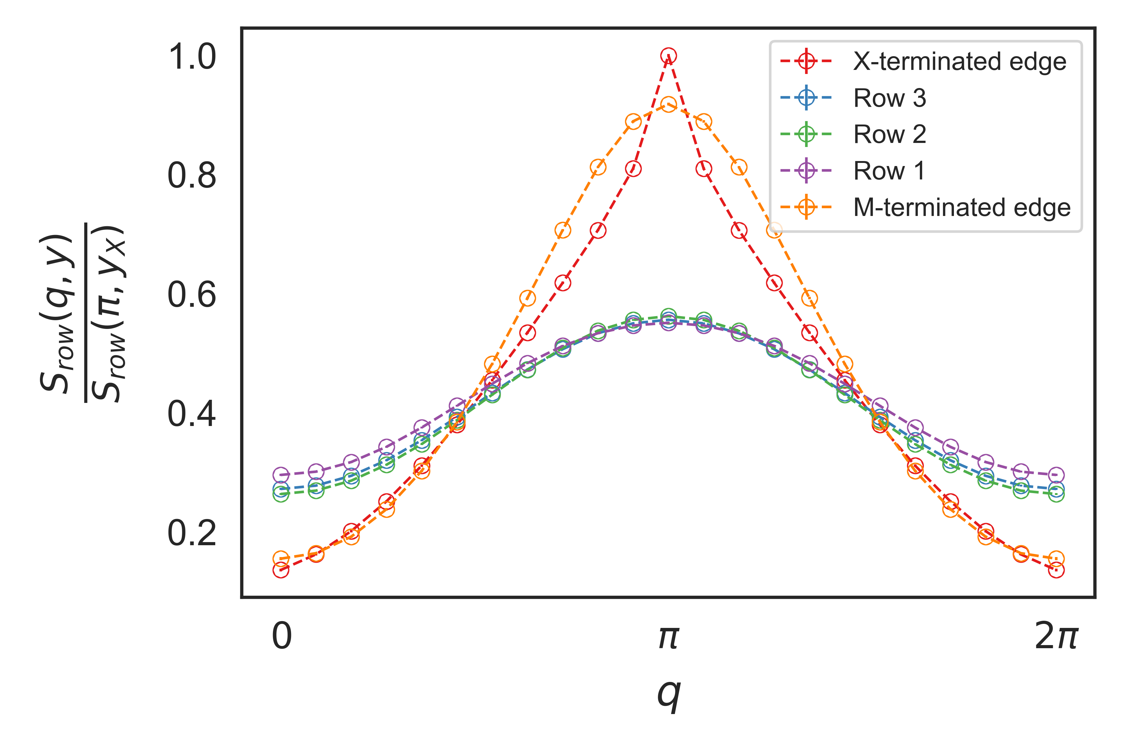
By varying the longitudinal dimension of the ribbon, , we are able to extrapolate the value of the staggered magnetization to the thermodynamic limit using the method outlined in Sec. II.2. In Fig. 12, we show finite-size scaling data for . On the top panel, one can see that the peak of sharpens as increases. On the bottom panel, it is seen that the staggered spin-spin correlation on the X- edge tends to a constant as the system size is increased, which signals antiferromagnetic ordering.


We find that the spin-spin correlations decay algebraically, indicating quasi long-range order. To fit the results, we use the power law:
| (14) |
where and are respectively the correlation length and the critical exponent, with and depending on whether is odd or even. By fitting to the DetQMC data for , we find the correlation lengths: and . These are consistent with our scaling hypothesis in Eq. (10) since . We also find the critical exponents and .
III.4 Comparison between MFT and DetQMC
We close this section with a critical comparison of the results obtained from MFT and DetQMC at , where the AF1 phase shows up. In order to obtain the staggered magnetization based on the DetQMC results, we plot for as a function of , and use Eq. (12) to extrapolate to the thermodynamic limit. Representative results are shown on the top panel of Fig. 13.


Notice that although we observe antiferromagnetic correlations at the M-edge with DetQMC, these do not signal magnetic ordering in the thermodynamic limit: the blue dashed line on the top panel intersects the -axis approximately at zero. It is possible that antiferromagnetism on the M-edge appears for higher values of similarly to what we observed with MFT. However, we cannot confirm this suspicion because the sign problem becomes too severe beyond (at which point our DetQMC simulations show no sign of antiferromagnetic order on the M-edge).
On the bottom panel of Fig. 13, we compare the extrapolated staggered magnetization obtained with DetQMC to the MFT results. We considered the same ribbon width in MFT but used . As expected, DetQMC predicts a higher critical interaction, , compared to the MFT result, . The agreement becomes better if we consider wider ribbons and/or in the MFT calculation. Qualitatively, the MFT and DetQMC results are similar in the sense that edge-antiferromagnetic ordering is established for values of the interaction that are of the same order of the band gap , with MFT overestimating long-range ordering. DetQMC unveils quasi-long-range order, with algebraic behavior of the spin-spin correlations.
IV Discussion and conclusions
We have used MFT and DetQMC to probe edge magnetism in zTMDNRs via a minimal three-band Hubbard model. Three main questions have been addressed: (1) How does changing the edge filling affect the phase diagram? (2) What is the effect of multiorbital interactions? (3) Can we use the numerically exact DetQMC approach to probe edge magnetism in TMD nanoribbons in spite of the well known sign problem?
To answer the first question, we considered an intraorbital Hubbard interaction, which we treated at the mean field level. We found two gapped phases: an edge-dimer phase (AF2), when the edges are half filled, and an edge-antiferromagnetic phase (AF1) at three-quarter edge filling. For other edge fillings, there is a tendency towards edge-ferromagnetism. As shown in Fig. 6, the ferromagnetic phases are metallic and the edge magnetization depends on the edge filling. Such magnetic edge states give rise to spin-polarized edge currents which could be tuned by changing the Fermi level through a back gate voltage. In particular, when the gapped phases are reached, these currents are suppressed. Similar behavior has been explored in zTMDNRs in the presence of magnetic proximity effect produced by ferromagnetic Cortés et al. 2019; Correa et al. 2020 and antiferromagnetic Cortés et al. 2020 substrates. Our results indicate that intrinsic magnetism could also be used to induce spin-polarized edge currents.
The second question has been answered by considering not only the intraorbital Hubbard interaction, but also an interorbital interaction term , as well as Hund and pair-hopping terms, characteristic of transition metal atoms. Within MFT, we obtained rich phase diagrams shown in Fig. 8, which corroborate and further complement the phases obtained with the simpler intraorbital Hubbard interaction. Generically, the interorbital term tends to suppress the magnetic phases, while and tend to enhance them. However, there are fillings for which stabilizes the ferromagnetic phase in a large portion of the phase diagram, as shown in Fig. 8(d).
As far as the third question is concerned, we have successfully applied DetQMC to the intraorbital Hubbard model for zTMDNRs, finding that edge magnetism strongly depends on the edge filling. In particular, at three-quarter edge filling – where the AF1 phase appears at mean field level – DetQMC has only a moderate sign problem and accurate results can be obtained. We have found edge-antiferromagnetic quasi-long-range order with spin-spin correlations behaving algebraically, reinforcing the AF1 phase predicted by MFT. The extrapolated staggered magnetization from DetQMC is consistent with the MFT result, as shown in Fig. 13. Even though in MFT long-range order is slightly overestimated, DetQMC and MFT agree that antiferromagnetism is more robust on the X-edge.
Let us point out that the dependence of edge magnetism on edge filling that we found might be relevant when interpreting experimental results. Often, the density of zigzag edges is used to explain how the ferromagnetic response varies between different nanosheet samples. Our results point to the edge filling as yet another key ingredient, since structural defects or chemisorbed adatoms may effectively change the filling of the edge. Finally, an important aspect for further study is the impact of a magnetic substrate — which induces magnetic exchange fields as considered in Refs. Cortés et al. 2019; Correa et al. 2020; Cortés et al. 2020 — on the edge magnetism of zTMDNRs. The methods we use in this work could be used to determine whether the edge magnetism we have found survives the presence of a substrate, and whether phase transitions can be induced by tuning the coupling to the substrate. Searching for edge magnetism at twin grain boundaries in 2D TMDs Čadež et al. 2019 and at 1D interface-states in TMD heterostructures Ávalos-Ovando et al. 2019 is another interesting direction.
V acknowledgements
We acknowledge support by the Portuguese Foundation for Science and Technology through Strategic Funding No. UIDB/04650/2020, Project No. POCI-01-0145-FEDER-028887. F.M.O.B. is supported by a DTP studentship funded by the Engineering and Physical Sciences Research Council. The authors would like to gratefully acknowledge João Pedro dos Santos Pires and Simão Meneses João for the enlightening discussions. This project was undertaken on the Viking Cluster, which is a high-performance computing facility provided by the University of York. We are grateful for computational support from the University of York High Performance Computing service (Viking) and the Research Computing team.
Appendix A Effect of edge bandwidth on edge magnetism
In this appendix, we discuss the impact of using different TMDs in our calculations, therefore changing the edge bandwidth, i.e., the portion of the spectrum corresponding to edge bands. Using different TMDs has only a slight impact on the edge magnetic ordering because the edge bandwidth is similar ( eV) among group 6 TMDs, as we show in Fig. 2.


We obtain the edge antiferromagnetic phases AF2 and AF1, respectively at for all the TMDs we considered. For other edge fillings, we find edge ferromagnetism. Even though there are slight differences in the specific values of the order parameters on each edge between the TMDs, our general qualitative conclusions do not change. We illustrate this for the AF1 phase in the top panel of Fig. 14. Notice that for and the two edges have the same value of the staggered magnetization. This is because these two TMDs have the narrowest edge bandwidths. Thus, for this specific Hubbard-, the magnetizations are likely already saturated, i.e. they have already reached their maximum value. On the bottom panel of Fig. 14, we show an example of the aforementioned edge antiferromagnetic phases for .
Appendix B Determinant Quantum Monte Carlo method
This appendix contains a brief description of our implementation of the DetQMC method that was used throughout this work and is publicly available at 11 1 DetQMC implementation, https://github.com/fmonteir/tmd-nanoribbon-detQMC, [Accessed: 20-March-2022]. Extensive details and bench-marking of the implementation are also available in Ref.Brito 2018. In order to enable the reader to reproduce our results, we focus on the aspects that are most relevant to this work. In particular, we provide details on how to write the spin correlation operator in terms of the Green’s functions, which are the main object of DetQMC simulations. In theory, expectations of quantum observables can be computed directly from the partition function. Unfortunately, it is not possible to obtain an explicit closed form expression for the latter for the interacting systems in this work. Thus DetQMC makes use of Monte Carlo sampling to compute expectations of the spin correlation operator.
In the path integral formulation, with discretized imaginary time, the partition function contains a product of exponential functions of a sum of non-commuting operators. This product can be approximated by using the Trotter breakup. Dividing the imaginary time interval into equal sub-intervals of smaller width , and using the inverse of the Baker–Campbell–Hausdorff formula, whilst keeping only the first order term in , we obtain
| (15) |
where is the three-band tight-binding Hamiltonian and is the intraorbital Hubbard term defined in the Hilbert space of the -th imaginary time slice. The parameter can be regarded as a high energy cutoff, and it must be larger than all other energy scales in the problem for the approximation to be valid.
Let us define the so called Hubbard Stratonovich (HS) binary field as a -dimensional, spin- field comprised of binary variables. The interaction term is eliminated by use of the discrete HS transformation for Bai et al. 2009; Hirsch 1983 . Since , we have
| (16) |
We will recast Eq.(16) in terms of the local electronic spin , yielding a non-interacting quadratic term. Let and . Introducing the binary variables , the discrete HST
| (17) |
allows one to write the exponential of the Hubbard term as a trace over the field at imaginary time slice Bai et al. 2009. In principle, a more complicated transformation could allow one to simulate the model with interorbital, Hund and pair-hopping terms. However, it would require three spin- fields Huang et al., thereby significantly increasing the computational cost, which is already quite high due to the sign problem. Moreover, such a transformation would likely lead to a more severe sign problem Held and Vollhardt 1998, increasing the computational cost even more or impeding simulations altogether. For the sake of simplicity and to avoid excessive computational cost, we have only included the intraorbital term in our simulations.
Let us define , with . Now, define HS fields for each imaginary time slice , which in turn specifies and . Including the trace over the field and exchanging it with the fermionic trace in Eq.(15), we obtain
| (18) |
where all operators are now quadratic in the fermion operators. For the latter, the trace over the electronic degrees of freedom may be taken explicitly Hanke et al. 1993, turning the many-fermion problem into a single-particle problem:
| (19) |
To multiply the chains of -matrices in a numerically stable manner, we use QR decompositions with partial pivoting Hanke et al. 1993; Bai et al. 2009; Bai et al. 2011. The determinant can be calculated in flops for a matrix whose size is polynomial in the number of sites , leading to a naive algorithm. To sample configurations of , we use single spin-flip dynamics. The acceptance/rejection scheme of the Metropolis algorithm is implemented using a rank-one update of the matrices Bai et al. 2009, which reduces the complexity of the algorithm to order . Using Wick’s theorem, we may write any observable in terms of the matrix elements of the Green’s function for a fixed configuration of the HS field, which in turn is given by Hanke et al. 1993; Bai et al. 2009. We use the Green’s function — the fundamental object of DetQMC — to sample configurations of the field and to measure spin correlations. We do so by averaging the spin correlation operator over uncorrelated configurations of the HS field to obtain an estimator of , the spin correlation between site/orbital pairs and . For each configuration, we measure the observable , defined in terms of as
| (20) |
A final remark must be made about computational effort. These simulations are plagued by the sign problem — which exponentially increases the variance of our estimators — deeming them very computationally intensive. In order to give the reader a concrete idea of just how intensive these simulations are, we compared two of the points shown in Fig. 9: we fixed and compared the data points shown for . Since the average sign for () is lower than for (), we expected to need more CPU hours in the case of the former in order to obtain similar accuracy to the case of the latter. This expectation was confirmed: 2930 CPU hours were required in order to obtain an error of in the electron density for , whilst 26093 CPU hours (almost 9 times more) were required in order to obtain an error of for . The data points were chosen to illustrate the computational cost because they were some of the most statistically demanding parts of this study.
References
- Manzeli et al. (2017) S. Manzeli, D. Ovchinnikov, D. Pasquier, O. V. Yazyev, and A. Kis, Nat. Rev. Mater. 2, 17033 (2017).
- Radisavljevic et al. (2011) B. Radisavljevic, A. Radenovic, J. Brivio, V. Giacometti, and A. Kis, Nat. Nanotechnol. 6, 147 (2011).
- Koppens et al. (2014) F. H. L. Koppens, T. Mueller, P. Avouris, A. C. Ferrari, M. S. Vitiello, and M. Polini, Nat. Nanotechnol. 9, 780 (2014).
- Mak and Shan (2016) K. F. Mak and J. Shan, Nat. Photonics 10, 216 (2016).
- Zhang et al. (2009) Y. Zhang, T.-T. Tang, C. Girit, Z. Hao, M. C. Martin, A. Zettl, M. F. Crommie, Y. R. Shen, and F. Wang, Nature 459, 820 (2009).
- Mak et al. (2010) K. F. Mak, C. Lee, J. Hone, J. Shan, and T. F. Heinz, Phys. Rev. Lett. 105, 136805 (2010).
- Tian et al. (2016) H. Tian, M. L. Chin, S. Najmaei, Q. Guo, F. Xia, H. Wang, and M. Dubey, Nano Res. 9, 1543 (2016).
- Khan and Leuenberger (2018) M. Khan and M. N. Leuenberger, Nanophotonics 7, 1589 (2018).
- Barthelmi et al. (2020) K. Barthelmi, J. Klein, A. Hötger, L. Sigl, F. Sigger, E. Mitterreiter, S. Rey, S. Gyger, M. Lorke, M. Florian, F. Jahnke, T. Taniguchi, K. Watanabe, V. Zwiller, K. D. Jöns, U. Wurstbauer, C. Kastl, A. Weber-Bargioni, J. J. Finley, K. Müller, and A. W. Holleitner, Appl. Phys. Lett. 117, 070501 (2020).
- Xiao et al. (2012) D. Xiao, G.-B. Liu, W. Feng, X. Xu, and W. Yao, Phys. Rev. Lett. 108, 196802 (2012).
- Schaibley et al. (2016) J. R. Schaibley, H. Yu, G. Clark, P. Rivera, J. S. Ross, K. L. Seyler, W. Yao, and X. Xu, Nat. Rev. Mater. 1, 16055 (2016).
- Enaldiev (2017) V. V. Enaldiev, Phys. Rev. B 96, 235429 (2017).
- Ciccarino et al. (2018) C. J. Ciccarino, T. Christensen, R. Sundararaman, and P. Narang, Nano Lett. 18, 5709 (2018).
- Zhou et al. (2019) B. T. Zhou, K. Taguchi, Y. Kawaguchi, Y. Tanaka, and K. T. Law, Commun. Phys. 2, 26 (2019).
- Molas et al. (2019) M. R. Molas, A. O. Slobodeniuk, T. Kazimierczuk, K. Nogajewski, M. Bartos, P. Kapuściński, K. Oreszczuk, K. Watanabe, T. Taniguchi, C. Faugeras, P. Kossacki, D. M. Basko, and M. Potemski, Phys. Rev. Lett. 123, 096803 (2019).
- Fujita et al. (1996) M. Fujita, K. Wakabayashi, K. Nakada, and K. Kusakabe, J. Phys. Soc. Jpn. 65, 1920 (1996).
- Wakabayashi et al. (1998) K. Wakabayashi, M. Sigrist, and M. Fujita, J. Phys. Soc. Jpn. 67, 2089 (1998).
- Yamashiro et al. (2003) A. Yamashiro, Y. Shimoi, K. Harigaya, and K. Wakabayashi, Phys. Rev. B 68, 193410 (2003).
- Son et al. (2006a) Y.-W. Son, M. L. Cohen, and S. G. Louie, Nature 444, 347 (2006a).
- Son et al. (2006b) Y.-W. Son, M. L. Cohen, and S. G. Louie, Phys. Rev. Lett. 97, 216803 (2006b).
- Rudberg et al. (2007) E. Rudberg, P. Sałek, and Y. Luo, Nano Lett. 7, 2211 (2007).
- Hod et al. (2007) O. Hod, V. Barone, J. E. Peralta, and G. E. Scuseria, Nano Lett. 7, 2295 (2007).
- Fernández-Rossier (2008) J. Fernández-Rossier, Phys. Rev. B 77, 075430 (2008).
- Jia et al. (2009) X. Jia, M. Hofmann, V. Meunier, B. G. Sumpter, J. Campos-Delgado, J. M. Romo-Herrera, H. Son, Y. P. Hsieh, A. Reina, J. Kong, M. Terrones, and M. S. Dresselhaus, Science 323, 1701 (2009).
- Jiao et al. (2009) L. Jiao, L. Zhang, X. Wang, G. Diankov, and H. Dai, Nature 458, 877 (2009).
- Tao et al. (2011) C. Tao, L. Jiao, O. V. Yazyev, Y.-C. Chen, J. Feng, X. Zhang, R. B. Capaz, J. M. Tour, A. Zettl, S. G. Louie, H. Dai, and M. F. Crommie, Nat. Phys. 7, 616 (2011).
- Nair et al. (2012) R. R. Nair, M. Sepioni, I.-L. Tsai, O. Lehtinen, J. Keinonen, A. V. Krasheninnikov, T. Thomson, A. K. Geim, and I. V. Grigorieva, Nat. Phys. 8, 199 (2012).
- Chen et al. (2021) C. Chen, Y. Lin, W. Zhou, M. Gong, Z. He, F. Shi, X. Li, J. Z. Wu, K. T. Lam, J. N. Wang, F. Yang, Q. Zeng, J. Guo, W. Gao, J. M. Zuo, J. Liu, G. Hong, A. L. Antaris, M. C. Lin, W. L. Mao, and H. Dai, Nat. Electron. 4, 653 (2021).
- Pizzochero and Kaxiras (2021) M. Pizzochero and E. Kaxiras, J. Phys. Chem. Lett. 12, 1214 (2021).
- Chen et al. (2017) Y. Chen, P. Cui, X. Ren, C. Zhang, C. Jin, Z. Zhang, and C.-K. Shih, Nat. Commun. 8, 15135 (2017).
- Cheng et al. (2017) F. Cheng, H. Xu, W. Xu, P. Zhou, J. Martin, and K. P. Loh, Nano Lett. 17, 1116 (2017).
- Li et al. (2018) S. Li, Y.-C. Lin, W. Zhao, J. Wu, Z. Wang, Z. Hu, Y. Shen, D.-M. Tang, J. Wang, Q. Zhang, H. Zhu, L. Chu, W. Zhao, C. Liu, Z. Sun, T. Taniguchi, M. Osada, W. Chen, Q.-H. Xu, A. T. S. Wee, K. Suenaga, F. Ding, and G. Eda, Nat. Mater. 17, 535 (2018).
- Wang et al. (2019) Z. Wang, X. Zhang, J. A. Hachtel, A. Apte, C. S. Tiwary, R. Vajtai, J. C. Idrobo, R. Ozturk, and P. Ajayan, Nanoscale Horiz. 4, 689 (2019).
- Yang et al. (2019) C. Yang, B. Wang, Y. Xie, Y. Zheng, and C. Jin, Nanotechnology 30, 255602 (2019).
- Munkhbat et al. (2020) B. Munkhbat, A. B. Yankovich, D. G. Baranov, R. Verre, E. Olsson, and T. O. Shegai, Nat. Commun. 11, 4604 (2020).
- Mao et al. (2013) X. Mao, Y. Xu, Q. Xue, W. Wang, and D. Gao, Nanoscale Res. Lett. 8, 430 (2013).
- Gao et al. (2013) D. Gao, M. Si, J. Li, J. Zhang, Z. Zhang, Z. Yang, and D. Xue, Nanoscale Res. Lett. 8, 129 (2013).
- Yang et al. (2015) Z. Yang, D. Gao, J. Zhang, Q. Xu, S. Shi, K. Tao, and D. Xue, Nanoscale 7, 650 (2015).
- Zhang et al. (2014) R. Zhang, Y. Li, J. Qi, and D. Gao, Nanoscale Res. Lett. 9, 586 (2014).
- Huo et al. (2014) N. Huo, Y. Li, J. Kang, R. Li, Q. Xia, and J. Li, Appl. Phys. Lett. 104, 202406 (2014).
- Kondo et al. (2017) G. Kondo, N. Yokoyama, S. Yamada, Y. Hashimoto, C. Ohata, S. Katsumoto, and J. Haruyama, AIP Adv. 7, 125019 (2017).
- Sarma et al. (2019) S. Sarma, B. Ghosh, S. C. Ray, H. T. Wang, T. S. Mahule, and W. F. Pong, J. Phys. Condens. Matter 31, 135501 (2019).
- Gao et al. (2017) G. Gao, C. Chen, X. Xie, Y. Su, S. Kang, G. Zhu, D. Gao, A. Trampert, and L. Cai, Mater. Res. Lett. 5, 267 (2017).
- Braz et al. (2018) J. E. H. Braz, B. Amorim, and E. V. Castro, Phys. Rev. B 98, 161406 (2018).
- Bollinger et al. (2001) M. V. Bollinger, J. V. Lauritsen, K. W. Jacobsen, J. K. Nørskov, S. Helveg, and F. Besenbacher, Phys. Rev. Lett. 87, 196803 (2001).
- Bollinger et al. (2003) M. V. Bollinger, K. W. Jacobsen, and J. K. Nørskov, Physical Review B 67, 085410 (2003).
- Li et al. (2008) Y. Li, Z. Zhou, S. Zhang, and Z. Chen, J. Am. Chem. Soc. 130, 16739 (2008).
- Vojvodic et al. (2009) A. Vojvodic, B. Hinnemann, and J. K. Nørskov, Phys. Rev. B 80, 125416 (2009).
- Botello-Méndez et al. (2009) A. R. Botello-Méndez, F. López-Urías, M. Terrones, and H. Terrones, Nanotechnology 20, 325703 (2009).
- Pan and Zhang (2012) H. Pan and Y.-W. Zhang, J. Mater. Chem. 22, 7280 (2012).
- Kou et al. (2012) L. Kou, C. Tang, Y. Zhang, T. Heine, C. Chen, and T. Frauenheim, J. Phys. Chem. Lett. 3, 2934 (2012).
- López-Urías et al. (2015) F. López-Urías, A. Laura Elías, N. Perea-López, H. R. Gutiérrez, M. Terrones, and H. Terrones, 2D Mater. 2, 015002 (2015).
- Cui et al. (2017) P. Cui, J. H. Choi, W. Chen, J. Zeng, C. K. Shih, Z. Li, and Z. Zhang, Nano Lett. 17, 1097 (2017).
- Vancsó et al. (2019) P. Vancsó, I. Hagymási, P. Castenetto, and P. Lambin, Phys. Rev. Mater. 3, 094003 (2019).
- Yang et al. (2016) G. Yang, S. Xu, W. Zhang, T. Ma, and C. Wu, Phys. Rev. B 94, 075106 (2016).
- Feldner et al. (2010) H. Feldner, Z. Y. Meng, A. Honecker, D. Cabra, S. Wessel, and F. F. Assaad, Phys. Rev. B 81, 115416 (2010).
- Feldner et al. (2011) H. Feldner, Z. Y. Meng, T. C. Lang, F. F. Assaad, S. Wessel, and A. Honecker, Phys. Rev. Lett. 106, 226401 (2011).
- Raczkowski and Assaad (2017) M. Raczkowski and F. F. Assaad, Phys. Rev. B 96, 115155 (2017).
- Yang et al. (2017) G. Yang, B. Li, W. Zhang, M. Ye, and T. Ma, J. Phys.: Condens. Matter 29, 365601 (2017).
- Shin et al. (2021) D. Shin, N. Tancogne-Dejean, J. Zhang, M. S. Okyay, A. Rubio, and N. Park, Phys. Rev. Lett. 126, 196406 (2021).
- Hirsch (1983) J. E. Hirsch, Phys. Rev. B 28, 4059 (1983).
- Blankenbecler et al. (1981) R. Blankenbecler, D. J. Scalapino, and R. L. Sugar, Phys. Rev. D 24, 2278 (1981).
- Hanke et al. (1993) W. Hanke, Y. V. Kopaev, and W. John, Cryst. Res. Technol. 28, 28 (1993).
- Liu et al. (2013) G.-B. Liu, W.-Y. Shan, Y. Yao, W. Yao, and D. Xiao, Phys. Rev. B 88, 085433 (2013).
- Chu et al. (2014) R.-L. Chu, G.-B. Liu, W. Yao, X. Xu, D. Xiao, and C. Zhang, Phys. Rev. B 89, 155317 (2014).
- Dagotto et al. (2001) E. Dagotto, T. Hotta, and A. Moreo, Phys. Rep. 344, 1 (2001).
- Ribic et al. (2014) T. Ribic, E. Assmann, A. Tóth, and K. Held, Phys. Rev. B 90, 165105 (2014).
- Mermin and Wagner (1966) N. D. Mermin and H. Wagner, Phys. Rev. Lett. 17, 1133 (1966).
- Varney et al. (2009) C. N. Varney, C.-R. Lee, Z. J. Bai, S. Chiesa, M. Jarrell, and R. T. Scalettar, Phys. Rev. B 80, 075116 (2009).
- Golor et al. (2013) M. Golor, T. C. Lang, and S. Wessel, Phys. Rev. B 87, 155441 (2013).
- Johnston et al. (2013) S. Johnston, E. A. Nowadnick, Y. F. Kung, B. Moritz, R. T. Scalettar, and T. P. Devereaux, Phys. Rev. B 87, 235133 (2013).
- Cheng et al. (2015) S. Cheng, J. Yu, T. Ma, and N. M. R. Peres, Phys. Rev. B 91, 075410 (2015).
- Troyer and Wiese (2005) M. Troyer and U.-J. Wiese, Phys. Rev. Lett. 94, 170201 (2005).
- Bai et al. (2009) Z. Bai, W. Chen, R. Scalettar, and I. Yamazaki, in Multi-Scale Phenomena in Complex Fluids, Series in Contemporary Applied Mathematics, Vol. 12 (World Scientific, Singapore, 2009) pp. 1–110.
- Roldán et al. (2013) R. Roldán, E. Cappelluti, and F. Guinea, Phys. Rev. B 88, 054515 (2013).
- Cortés et al. (2019) N. Cortés, O. Ávalos-Ovando, L. Rosales, P. Orellana, and S. Ulloa, Phys. Rev. Lett. 122, 086401 (2019).
- Correa et al. (2020) J. H. Correa, A. C. Dias, L. Villegas-Lelovsky, J. Fu, L. Chico, and F. Qu, Phys. Rev. B 101, 195422 (2020).
- Cortés et al. (2020) N. Cortés, O. Ávalos-Ovando, and S. E. Ulloa, Phys. Rev. B 101, 201108R (2020).
- Čadež et al. (2019) T. Čadež, L. Li, E. V. Castro, and J. M. P. Carmelo, Phys. Rev. B 99, 155109 (2019).
- Ávalos-Ovando et al. (2019) O. Ávalos-Ovando, D. Mastrogiuseppe, and S. E. Ulloa, J. Phys. Condens. Matter 31, 213001 (2019).
- (81) DetQMC implementation, https://github.com/fmonteir/tmd-nanoribbon-detQMC, [Accessed: 20-March-2022].
- Brito (2018) F. M. O. Brito, Master’s thesis, Instituto Superior Técnico (2018).
- (83) X.-X. Huang, B. Moritz, M. Claassen, and T. P. Devereaux, Phys. Rev. B 105, 165124.
- Held and Vollhardt (1998) K. Held and D. Vollhardt, Eur. Phys. J. B 5, 473 (1998).
- Bai et al. (2011) Z. Bai, C. Lee, R.-C. Li, and S. Xu, Linear Algebra and its Applications Special Issue: Dedication to Pete Stewart on the occasion of his 70th birthday, 435, 659 (2011).