Partial-Attribution Instance Segmentation for Astronomical Source Detection and Deblending
Abstract
Astronomical source deblending is the process of separating the contribution of individual stars or galaxies (sources) to an image comprised of multiple, possibly overlapping sources. Astronomical sources display a wide range of sizes and brightnesses and may show substantial overlap in images. Astronomical imaging data can further challenge off-the-shelf computer vision algorithms owing to its high dynamic range, low signal-to-noise ratio, and unconventional image format. These challenges make source deblending an open area of astronomical research, and in this work, we introduce a new approach called Partial-Attribution Instance Segmentation that enables source detection and deblending in a manner tractable for deep learning models. We provide a novel neural network implementation as a demonstration of the method.
1 Introduction
Astronomical images can contain tens of thousands of stars and galaxies (sources). Forthcoming telescopes including the Vera Rubin Observatory [11, 12], James Webb Space Telescope [26], and Nancy Grace Roman Space Telescope [24, 25] will push the current limits of observational astronomy and dramatically increase the number of sources to analyze. To measure accurate properties for these sources, we must detect sources by identifying statistically significant local maxima in an image and deblend sources by isolating the potentially overlapping flux distributions of each object. Consider a background-subtracted astronomical image in which sources are observed, where is the height, is the width, and indicates the number of astronomical passbands. The image can be decomposed into a sum of individual object contributions as
| (1) |
where represents the flux contributed to by source , and is the approximate noise distribution in the image. The process of decomposing an image into the form of Equation 1 represents the core challenge of source deblending. This submission presents a deep learning-based method to perform detection and deblending on astronomical images.
1.1 Related Work
Source detection and deblending are well-studied problems in astronomy, and many approaches have been developed. Below, we highlight some popular and recent methods for source detection and deblending and point the interested reader to the review by Masias et al. 2012.
Detection and deblending methods can be characterized by their detection capacity and deblend type. The detection capacity represents the number of sources a method can detect within a single image. For Equation 1, a detection capacity of would indicate that a method could detect all sources appearing in an image. The deblend type indicates how the flux in a single pixel may be split between overlapping (blended) sources. A disjoint deblender assigns all flux in a pixel to a single source exclusively. An intersecting/discrete deblender can assign the flux to more than one source with uniform weighting across pixels. Finally, an intersecting/continuous deblender can assign the flux to more than one source with variable weighting across pixels.
Astronomical analysis methods vary in their detection and deblending methods. Bertin & Arnouts 1996 introduced SExtractor that uses a convolution and thresholding approach for detection, and an isophotal analysis using binned pixel intensity for deblending. Hausen & Robertson 2020 introduced Morpheus, a U-Net [23] style convolutional neural network (CNN) model that filters out background pixels, uses a thresholding approach for detection, and combines watershed and peak finding algorithms for deblending. Another U-Net based model called blend2mask [3] performs detection and deblending using the U-Net alone. Reiman & Göhre 2019 use a modified Super-Resolution GAN (SRGAN) [16] to deblend overlapping sources. Burke et al. 2019 trained a Mask R-CNN [8] model to detect and deblend sources. SCARLET [19] deblends sources using constrained matrix factorization.
Table 1 summarizes the features of these previous methods, none of which have a detection capacity of and an intersecting/continuous deblend type. We now present a deep learning-based intersecting/continuous deblending algorithm with a detection capacity of .
| Name | Detection Capacity | Deblend Type |
|---|---|---|
| SExtractor[2] | Disjoint | |
| Morpheus[7] | Disjoint | |
| Mask R-CNN[4] | Intersecting/Discrete | |
| blend2mask2flux[3] | Intersecting/Discrete | |
| Modified SRGAN[22] | 0 | Intersecting/Continuous |
| SCARLET[19] | 0 | Intersecting/Continuous |
| This Work | Intersecting/Continuous |
2 Partial-Attribution Instance Segmentation
Partial-Attribution Instance Segmentation (PAIS) is a new extension of the instance segmentation paradigm that allows for weighted, overlapping segmentation maps. PAIS differs from other segmentation schemes like cell segmentation [28], interacting surface segmentation [27], and amodal instance segmentation [17]. PAIS aims to isolate objects appearing in an image while preserving their measurable quantities within areas of overlap. For PAIS, we can approximate Equation 1 as
| (2) |
where estimates the background-subtracted flux image in Equation 1, constitutes the pixel-level fractional contribution of source to , and symbolizes the Hadamard product. Equation 2 is tractable for deep learning models, allowing the model to learn the bounded quantities rather than the unbounded source images . The number of sources setting the upper limit of the sum in Equation 2 can differ for each image.
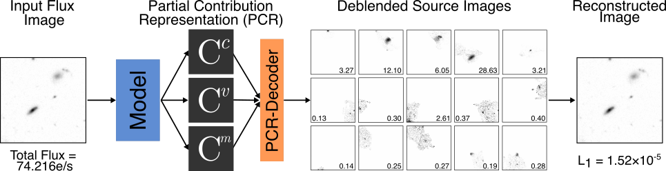
To construct a PAIS format that can be represented by a CNN, we have to construct an encoding for the in Equation 2. Inspired by Cheng et al. 2019 and Kendall et al. 2017, we propose an encoding for the components called Partial Contribution Representation (PCR). The goal of PCR is to encode, for any single pixel , the fractional contribution to its intensity from the closest sources. Using PCR, a variable number of sources can be encoded per image. PCR consists of three tensors: the Center-of-mass , Contribution-vectors and Contribution-maps . The center-of-mass encodes the locations of all the sources in an image. For any pixel, we set if that location indicates the center of a source and otherwise. The contribution-vector encodes the Cartesian offset to the closest sources. The contribution-map connects the fractional contribution of the sources with the associated contribution-vectors . The fixed dimensionality of , , and make PCR tractable for deep learning algorithms.
3 Our Approach
Our approach consists of making a PAIS dataset leveraging PCR and is implemented using a novel neural network architecture. We summarize our dataset, model, and training method below.
3.1 Dataset
To generate the PAIS input samples, we used the Hubble Legacy Fields (HLF) GOODS-South F160W () flux images [10], along with the 3D-HST source catalog [20]. The HLF images were split into training and test sets of pixel subregions, with 2,000 training samples and 500 test samples. The input labels, as described in Section 2, consist of the center-of-mass images , the contribution-vectors , and the contribution-maps . The center-of-mass training images are generated in a manner similar to Cheng et al. 2019, by placing pixelated 2D Gaussians with standard deviation at the locations of sources in the 3D-HST catalog. The contribution-vectors, an extension to the method by Cheng et al. 2019, are generated from the Cartesian offset to the nearest sources to each pixel. The contribution-maps require the values from Equation 2. To determine , we use SCARLET [19] with the F125W, F160W, F606W, and F850LP flux and weight images from the HLF GOODS-South data and the TinyTim point-spread functions [15] to deblend the sources from the 3D-HST catalog. We then use PCR to encode the from SCARLET. The complete dataset generation routine can be found in our project repository (https://github.com/ryanhausen/morpheus-deblend/ ).
To evaluate the efficacy of PCR to encode , we define two metrics. We use the mean difference between the total flux determined by the SCARLET encoded for each input source and that recovered by our encoding. We also use a two-sample Kolmogorov–Smirnov (KS) test to compare the normalized cumulative surface brightness profile within the radius encompassing 90% of the total flux of each source to evaluate the encoding of the spatial flux distribution. Table 2 reports the results and demonstrates that PCR encoding approximately preserves both the total flux and the spatial flux distribution for each source. With this verification, we can train a network to recover the PCR encoding for each input HST F160W image.
| Test | Value |
|---|---|
| Total Source Flux [e/s] (MAE) | |
| Two-Sample KS Test p-value |
3.2 Model
To recover the PCR for training images, we developed a novel neural network architecture inspired by Cheng et al. 2019, based on the Fast Attention Network [9] and implemented in TensorFlow [1]. The model features two decoders that share a single encoder. The first decoder, called the spatial decoder, predicts values for and . The second decoder, called the attribution decoder, predicts values for . The complete model code can be found in the repository for this project (https://github.com/ryanhausen/morpheus-deblend/ ). An end-to-end example of the model can be seen in Figure 1.
3.3 Training
To train the model to recover the PCR of the input images, we use the Adam Optimizer [14] with a learning rate of , , , , and a batch size of 100. The model was trained for 1000 epochs using an NVIDIA V100 32GB GPU, taking 31 hours. The loss function for the model is composed of three functions. The spatial decoder outputs for and are penalized according to mean squared error (MSE) and the mean absolute error (MAE), respectively. The attribution decoder output is penalized using cross-entropy loss with an additional entropy regularization term. In practice, we found that the additional entropy regularization helped incentivize the network to learn information about multiple sources in . Each loss term is weighted and combined into a single loss function described by
| (3) |
where is the MSE loss calculated between the model output and input label with , is the MAE loss calculated between the model output and input label with , is a cross-entropy loss calculated between the model output and input label with , and is the entropy regularization on the model output with . See Table 3 for a summary of the training results, demonstrating a good balance between test and training error. A complete log of training experiments is available at (https://www.comet.ml/ryanhausen/morpheus-deblend/ ).
| Metric | Training | Test |
|---|---|---|
| MAE | ||
| MSE | ||
| cross-entropy |
4 Discussion and Future Work
In this work, we introduced the Partial Attribution Instance Segmentation (PAIS) scheme for astronomical source debelending. We presented Partial Contribution Representation (PCR) as a method for implementing PAIS within deep learning-based models. We demonstrated the efficacy of PCR for encoding the results of existing astronomical deblenders, and developed a novel neural network architecture to recover the PCR from input flux images. While we demonstrated deblending for single band (F160W) images, PCR can be extended to multiband images. As with many supervised methods, our model requires labeled training data. To apply this method on other survey datasets may require the use of transfer learning [6, 21] or retraining.
Acknowledgments and Disclosure of Funding
5 Acknowledgements
RDH would like to thank Roberto Manduchi for helpful conversations. BER acknowledges support from NASA contract NNG16PJ25C and grant 80NSSC18K0563. The authors acknowledge use of the lux supercomputer at UC Santa Cruz, funded by NSF MRI grant AST 1828315.
6 Broader Impact
This work develops a novel method for separating source signals in astronomical images. Due to the specialized format and problem setting, the authors do not see any broader negative societal impacts as a result of this work.
References
- Abadi et al. [2016] Abadi, M., Agarwal, A., Barham, P., et al. 2016, arXiv e-prints, arXiv:1603.04467. https://arxiv.org/abs/1603.04467
- Bertin & Arnouts [1996] Bertin, E., & Arnouts, S. 1996, A&AS, 117, 393, doi: 10.1051/aas:1996164
- Boucaud et al. [2020] Boucaud, A., Huertas-Company, M., Heneka, C., et al. 2020, MNRAS, 491, 2481, doi: 10.1093/mnras/stz3056
- Burke et al. [2019] Burke, C. J., Aleo, P. D., Chen, Y.-C., et al. 2019, MNRAS, 490, 3952, doi: 10.1093/mnras/stz2845
- Cheng et al. [2019] Cheng, B., Collins, M. D., Zhu, Y., et al. 2019, arXiv e-prints, arXiv:1911.10194. https://arxiv.org/abs/1911.10194
- Domínguez Sánchez et al. [2019] Domínguez Sánchez, H., Huertas-Company, M., Bernardi, M., et al. 2019, MNRAS, 484, 93, doi: 10.1093/mnras/sty3497
- Hausen & Robertson [2020] Hausen, R., & Robertson, B. E. 2020, ApJS, 248, 20, doi: 10.3847/1538-4365/ab8868
- He et al. [2017] He, K., Gkioxari, G., Dollár, P., & Girshick, R. 2017, arXiv e-prints, arXiv:1703.06870. https://arxiv.org/abs/1703.06870
- Hu et al. [2020] Hu, P., Perazzi, F., Caba Heilbron, F., et al. 2020, arXiv e-prints, arXiv:2007.03815. https://arxiv.org/abs/2007.03815
- Illingworth et al. [2016] Illingworth, G., Magee, D., Bouwens, R., et al. 2016, arXiv e-prints, arXiv:1606.00841. https://arxiv.org/abs/1606.00841
- Ivezić et al. [2008] Ivezić, Ž., Kahn, S. M., Tyson, J. A., et al. 2008, arXiv e-prints. https://arxiv.org/abs/0805.2366
- Ivezić et al. [2019] Ivezić, Ž., Kahn, S. M., Tyson, J. A., et al. 2019, ApJ, 873, 111, doi: 10.3847/1538-4357/ab042c
- Kendall et al. [2017] Kendall, A., Gal, Y., & Cipolla, R. 2017, arXiv e-prints, arXiv:1705.07115. https://arxiv.org/abs/1705.07115
- Kingma & Ba [2014] Kingma, D. P., & Ba, J. 2014, ArXiv e-prints. https://arxiv.org/abs/1412.6980
- Krist et al. [2011] Krist, J. E., Hook, R. N., & Stoehr, F. 2011, in Society of Photo-Optical Instrumentation Engineers (SPIE) Conference Series, Vol. 8127, Optical Modeling and Performance Predictions V, ed. M. A. Kahan, 81270J, doi: 10.1117/12.892762
- Ledig et al. [2016] Ledig, C., Theis, L., Huszar, F., et al. 2016, arXiv e-prints, arXiv:1609.04802. https://arxiv.org/abs/1609.04802
- Li & Malik [2016] Li, K., & Malik, J. 2016, arXiv e-prints, arXiv:1604.08202. https://arxiv.org/abs/1604.08202
- Masias et al. [2012] Masias, M., Freixenet, J., Lladó, X., & Peracaula, M. 2012, MNRAS, 422, 1674, doi: 10.1111/j.1365-2966.2012.20742.x
- Melchior et al. [2018] Melchior, P., Moolekamp, F., Jerdee, M., et al. 2018, Astronomy and Computing, 24, 129, doi: 10.1016/j.ascom.2018.07.001
- Momcheva et al. [2016] Momcheva, I. G., Brammer, G. B., van Dokkum, P. G., et al. 2016, ApJS, 225, 27, doi: 10.3847/0067-0049/225/2/27
- Pratt [1993] Pratt, L. Y. 1993, in Advances in Neural Information Processing Systems 5, ed. S. J. Hanson, J. D. Cowan, & C. L. Giles (Morgan-Kaufmann), 204–211. http://papers.nips.cc/paper/641-discriminability-based-transfer-between-neural-networks.pdf
- Reiman & Göhre [2019] Reiman, D. M., & Göhre, B. E. 2019, MNRAS, 485, 2617, doi: 10.1093/mnras/stz575
- Ronneberger et al. [2015] Ronneberger, O., Fischer, P., & Brox, T. 2015, arXiv e-prints, arXiv:1505.04597. https://arxiv.org/abs/1505.04597
- Spergel et al. [2013] Spergel, D., Gehrels, N., Breckinridge, J., et al. 2013, arXiv e-prints, arXiv:1305.5422. https://arxiv.org/abs/1305.5422
- Spergel et al. [2015] Spergel, D., Gehrels, N., Baltay, C., et al. 2015, arXiv e-prints, arXiv:1503.03757. https://arxiv.org/abs/1503.03757
- Williams et al. [2018] Williams, C. C., Curtis-Lake, E., Hainline, K. N., et al. 2018, ApJS, 236, 33, doi: 10.3847/1538-4365/aabcbb
- Xie et al. [2020] Xie, H., Pan, Z., Zhou, L., et al. 2020, arXiv e-prints, arXiv:2007.01259. https://arxiv.org/abs/2007.01259
- Zhou et al. [2020] Zhou, Y., Chen, H., Lin, H., & Heng, P.-A. 2020, arXiv e-prints, arXiv:2007.10787. https://arxiv.org/abs/2007.10787