跳到论文正文
W Papers独立论文阅读器 arXiv:2201.04545 论文正文 计算阅读时间 · 0%
引用这篇论文根据当前论文元数据生成,正式投稿前建议核对。


License: CC BY 4.0
arXiv:2201.04545v3 [stat.ML] 16 Oct 2022

On Generalization Bounds for Deep Networks
based on Loss Surface Implicit Regularization

Masaaki Imaizumi    Johannes Schmidt-Hieber Thanks:  Masaaki Imaizumi received support from JSPS KAKENHI (18K18114) and JST Presto (JPMJPR1852). Johannes Schmidt-Hieber received support from the Dutch Science Foundation (NWO) via the Vidi grant VI.Vidi.192.021. Masaaki Imaizumi is with Komaba Institute for Science, the University of Tokyo, Japan. (e-mail imaizumi@g.ecc.u-tokyo.ac.jp) Johannes Schmidt-Hieber is with the University of Twente, Netherlands. (e-mail a.j.schmidt-hieber@utwente.nl)
August 11, 2026
Abstract

The classical statistical learning theory implies that fitting too many parameters leads to overfitting and poor performance. That modern deep neural networks generalize well despite a large number of parameters contradicts this finding and constitutes a major unsolved problem towards explaining the success of deep learning. While previous work focuses on the implicit regularization induced by stochastic gradient descent (SGD), we study here how the local geometry of the energy landscape around local minima affects the statistical properties of SGD with Gaussian gradient noise. We argue that under reasonable assumptions, the local geometry forces SGD to stay close to a low dimensional subspace and that this induces another form of implicit regularization and results in tighter bounds on the generalization error for deep neural networks. To derive generalization error bounds for neural networks, we first introduce a notion of stagnation sets around the local minima and impose a local essential convexity property of the population risk. Under these conditions, lower bounds for SGD to remain in these stagnation sets are derived. If stagnation occurs, we derive a bound on the generalization error of deep neural networks involving the spectral norms of the weight matrices but not the number of network parameters. Technically, our proofs are based on controlling the change of parameter values in the SGD iterates and local uniform convergence of the empirical loss functions based on the entropy of suitable neighborhoods around local minima.

Index Terms: 
deep neural network, generalization error, uniform convergence, non-convex optimization

I Introduction

We consider supervised learning using deep neural networks. Let (X1,Y1),…,(Xn,Yn)(X_{1},Y_{1}),...,(X_{n},Y_{n}) be nn i.i.d. observed pairs in 𝒳×𝒴\mathcal{X}\times\mathcal{Y} with input space 𝒳\mathcal{X} and output space 𝒴\mathcal{Y}. Write f⁡(⋅,𝒜):𝒳→𝒴f(\cdot;\mathcal{A}):\mathcal{X}\to\mathcal{Y} for a function generated by a neural network with LL layers and parameter matrices 𝒜=(A1,…,AL).\mathcal{A}=(A_{1},...,A_{L}). The total number of parameters is denoted by D.D. We assume that the set of possible network parameters is constrained to lie in a known parameter space Θ⊆ℝD.\Theta\subseteq\mathbb{R}^{D}. Let ℓ:𝒴×𝒴→ℝ\ell:\mathcal{Y}\times\mathcal{Y}\to\mathbb{R} be the loss function and denote by 𝒜^\widehat{\mathcal{A}} the output of the stochastic gradient descent (SGD) algorithm based on the empirical loss Rn​(𝒜):=n−1​∑i=1nℓ⁡(Yi,f⁡(Xi,𝒜)).R_{n}(\mathcal{A}):=n^{-1}\sum_{i=1}^{n}\ell(Y_{i},f(X_{i};\mathcal{A})). The expected loss (generalization error) is then given by R⁡(𝒜):=𝔼⁡[ℓ⁡(Y,f⁡(X,𝒜))]R(\mathcal{A}):=\mathbb{E}[\ell(Y,f(X;\mathcal{A}))]. Throughout this manuscript, we assume that the loss if sufficiently regular such that the gradient ∇R​(𝒜)\nabla R(\mathcal{A}) exists for all 𝒜\mathcal{A}.

To achieve small generalization error, we are interested in bounds for the generalization gap

R​(𝒜^)−Rn​(𝒜^)\displaystyle R(\widehat{\mathcal{A}})-R_{n}(\widehat{\mathcal{A}})

with 𝒜^\widehat{\mathcal{A}} the SGD output. In this work, we derive a new bound for the generalization gap, by exploiting the tendency of SGD iterates to stay in neighborhoods of critical points in the loss surface. We then argue that for complex loss surfaces, this constraints the SGD iterates considerably and leads to implicit regularization. Throughout this article we refer to this type of implicit regularization as loss surface implicit regularization.

I-A Background

Deep learning is known to achieve outstanding performance in various complicated tasks, such as image recognition, text analysis, and reinforcement learning [1]. For some tasks, super-human performance has been reported [2, 3, 4]. Despite the impressive practical performance, there is still a gap regarding the theoretical understanding of deep learning. Obstacles in the theoretical foundation include the higher-order nonlinear structures due to the stacking of multiple layers and the excessive number of network parameters in state of the art networks. For some recent surveys, see [5, 6].

To understand the use of fitting large numbers of parameters, requires to rethink generalization [7]. Indeed, according to the standard statistical learning theory, large models overfit and thus increase the generalization error. Based on the classical analysis (e.g., the textbook [8]), the generalization gap for deep neural networks with LL layers and DD parameters is of the order

R⁡(𝒜^)−Rn​(𝒜^)=O~ℙ​(L​D/n)\displaystyle R(\widehat{\mathcal{A}})-R_{n}(\widehat{\mathcal{A}})=\widetilde{O}_{\mathbb{P}}(\sqrt{{LD}/{n}})

where O~ℙ​(⋅)\widetilde{O}_{\mathbb{P}}(\cdot) stands for the Big O notation ignoring logarithmic factors and the index ℙ\mathbb{P} indicates that the rates are in probability. While bounds of this type can be used to prove optimal statistical convergence rates for sparsely connected neural networks [9, 10, 11, 12], the bound is clearly not sharp enough to explain the success of fully connected highly overparametrized models. Hence, a new theoretical framework is needed.

One possibility to derive sharper bounds on the generalization gap is to take the implicit regularization into account. Learning algorithms, such as SGD, implicitly regularize and constraint the degrees of freedom. In several specific models, including linear regression, logistic regression and linear neural networks, it has been shown that gradient descent methods converges to interpolants with minimum norm constraints [13, 14, 15, 16, 17, 18, 19, 20]. Motivated by this fact, several articles investigate the generalization gap under the assumption that a norm on the network parameters is bounded by a threshold. For example, [21] assumes that the network parameters lie in a norm-bounded subset ℬ~:={𝒜=(A1,…,AL)∣∥Aℓ∥F≤bℓ,ℓ=1,…,L}⊂Θ\widetilde{\mathcal{B}}:=\left\{\mathcal{A}=(A_{1},...,A_{L})\mid\|A_{\ell}\|_{F}\leq b_{\ell},\ell=1,...,L\right\}\subset\Theta with b1,…,bLb_{1},\dots,b_{L} given and ∥⋅∥F\|\cdot\|_{F} the Frobenius norm. It is shown that the generalization gap is then R⁡(𝒜^)−Rn​(𝒜^)=O~ℙ​(2L​Πℓ=1L​bℓ/n).R(\widehat{\mathcal{A}})-R_{n}(\widehat{\mathcal{A}})=\widetilde{O}_{\mathbb{P}}\left({2^{L}\Pi_{\ell=1}^{L}b_{\ell}}/{\sqrt{n}}\right). Interestingly, the bound only depends on the number of layers LL, the number of training data nn and the radii bℓ,b_{\ell}, but not on the number of network parameters. This shows that norm control can avoid overfitting even in the case of overparametrization. [22] derives the generalization gap bound R⁡(𝒜^)−Rn​(𝒜^)=O~ℙ​(Πℓ=1L​sℓ​(∑ℓ=1L(bˇℓ/sℓ)2/3)3/2/n)R(\widehat{\mathcal{A}})-R_{n}(\widehat{\mathcal{A}})=\widetilde{O}_{\mathbb{P}}({\Pi_{\ell=1}^{L}s_{\ell}(\sum_{\ell=1}^{L}(\check{b}_{\ell}/s_{\ell})^{2/3})^{3/2}}/{\sqrt{n}}) for the set of network parameters ℬˇ:={𝒜=(A1,…,AL)\check{\mathcal{B}}:=\{\mathcal{A}=(A_{1},...,A_{L}) ∣∥Aℓ∥2,1≤bˇℓ,∥Aℓ∥s≤sℓ,ℓ=1,…,L},\mid\|A_{\ell}\|_{2,1}\leq\check{b}_{\ell},\|A_{\ell}\|_{s}\leq s_{\ell},\ell=1,...,L\}, where ‖A‖2,1\|A\|_{2,1} denotes the sum of the Euclidean norms of the rows of the matrix AA and ∥⋅∥s\|\cdot\|_{s} is the spectral norm. This bound has been extended and improved in subsequent work [23, 24]. Especially, [22] bounds the generalization gap by a product of the spectral norms of the parameter matrices. Alternatively, [25] derived a bound on the generalization gap involving the parameter distance between the initial value and a global minimizer. Section I-C provides a more comprehensive overview of related work.

The imposed constraints on the parameter norms might be violated in practice. [26] shows that during network training, the parameter matrices 𝒜\mathcal{A} move far away from the origin and the initialization. Empirically, it is argued that the distance to the initialization increases polynomially with the number of training data. The claim is that only for simple models, implicit regularization favors small norms.

I-B Summary of Results

We first define suitable neighborhoods around the local minima of the loss surface. Under a number of conditions, we then prove that SGD with Gaussian gradient noise enters such a neighborhood and will not escape it with positive probability. For this reason, we also call the neighborhoods stagnation sets. In a second step, we derive bounds for the complexity of these neighborhoods. Conditionally on the SGD iterates lying in one of these neighborhoods, we finally derive a generalization gap bound. Based on these results, we then argue that the loss surface itself constraints the SGD resulting in the loss surface implicit regularization.

To define a suitable notion of a stagnation set, we consider a sequence of parameters {𝒜t}t=1T\{\mathcal{A}_{t}\}_{t=1}^{T} generated by Gaussian SGD with an iteration index t∈ℕt\in\mathbb{N} and a stopping time T∈ℕ.T\in\mathbb{N}. The initial value is 𝒜0∈Θ\mathcal{A}_{0}\in\Theta and the iterates are defined via the update equation 𝒜t+1=𝒜t−ηt∇R^n(𝒜t)\mathcal{A}_{t+1}=\mathcal{A}_{t}-\eta_{t}\nabla\widehat{R}_{n}(\mathcal{A}_{t}). Here, ηt>0\eta_{t}>0 is a given learning rate and R^n\widehat{R}_{n} is a perturbed loss with Gaussian noise such that the updates resemble SGD (a formal definition is provided in (2)). The output of the method is 𝒜^=𝒜T\widehat{\mathcal{A}}=\mathcal{A}_{T}. We define the notion of a stagnation set as follows:

Definition 1 (Stagnation Set).

For p∈[0,1]p\in[0,1], ℬ⊂Θ\mathcal{B}\subset\Theta is a pp-stagnation set, if the following holds with some t¯≥1\bar{t}\geq 1:

ℙ(𝒜t∈ℬ,∀t∈[t¯,T])≥p.\displaystyle\mathbb{P}\left(\mathcal{A}_{t}\in\mathcal{B},\forall t\in[\bar{t},T]\right)\geq p.

For convenience, we omit the dependence on t¯\bar{t} and only indicate the dependence on pp in the notation of a pp-stagnation set. Indeed, the dependence on t¯\bar{t} is of little importance, as t¯\bar{t} is fixed and considered to be small compared to the total number of iterations T.T.

Thus with probability at least pp, SGD will not leave the set ℬ\mathcal{B} anymore. Conditionally on this event, it is sufficient to control the Rademacher complexity of ℬ\mathcal{B} to bound the generalization gap. On the contrary, a set is a 00-stagnation set if the output of the Gaussian SGD algorithm does not stagnate in the set. In this case, it is impossible to derive a generalization gap bound based on the Rademacher complexity of such a set. According to the empirical study in [26], SGD does not stagnate in the sets B~\tilde{B} or Bˇ\check{B} defined in Section I-A, implying that those are pp-stagnation set for some small pp or even p=0p=0.

Refer to caption
Refer to caption
Fig. 1: (Top) Contours of a two-dimensional projection of the test loss surface of a deep residual neural network with 5656 layers trained using CIFAR-10 data. For the training pruning of shortcuts is applied [2]. The two-dimensional projection is generated by dimension reduction of the 850,000850,000 dimensional parameter space using the random-direction method [27]. (Bottom) Population minima (red dots) and their neighbourhoods (blue balls) on the loss surface. Here the population minima are computed using the test data. For the visualization, the radius of all balls is set to 0.080.08 in the dimension-reduced space.

As illustrated in Figure 1, the loss landscape of neural networks is highly-nonconvex and possesses multiple local minima whose neighborhoods form attractive basins. Note that in the definition above, a stagnation set is non-random. As candidate for good stagnation sets, we take the union over local neighborhoods of the minima of the expected loss surface.

Definition 2 (Population Minimum).

We call a subset μ⊆Θ\mu\subseteq\Theta a population minimum, if μ\mu is a maximally connected set consisting of local minima of R⁡(𝒜)R(\mathcal{A}).

Let us emphasize again that those are minima of the expected loss surface and not the empirical loss surface. Consequently, the set μ\mu is deterministic. To see why a minimum does not simply consists of one parameter as in the case of a strictly convex loss surface, consider a ReLU network with activation function σ⁡(x)=max⁡(x,0).\sigma(x)=\max(x,0). Multiplying all parameters in one hidden layer of a ReLU network by α>0\alpha>0 and dividing in another hidden layer all parameters by 1/α,1/\alpha, gives the same network function. Thus, if 𝒜=(A1,…,AL)∈μ\mathcal{A}=(A_{1},\ldots,A_{L})\in\mu then also 𝒜′=(α​A1,α−1​A2,A3,…,AL)∈μ.\mathcal{A}^{\prime}=(\alpha A_{1},\alpha^{-1}A_{2},A_{3},\ldots,A_{L})\in\mu. For general activation function, if a minimum corresponds to a parameter 𝒜=(A1,…,AL)\mathcal{A}=(A_{1},\ldots,A_{L}) such that one of the weight matrices AℓA_{\ell} has a zero column vector, then, some of the parameters of the previous layer Aℓ−1A_{\ell-1} do not affect the loss function. Hence, the population minimum can in principle consist of several parameters, regardless of the choice of activation function.

In Definition 3, we introduce a suitable notion of δ\delta-neighborhood around μ,\mu, denoted by ℬδ​(μ)⊂Θ.\mathcal{B}_{\delta}(\mu)\subset\Theta. A key object in our approach is the union of δ\delta-neighbourhoods over several minima μ1,…,μK\mu_{1},...,\mu_{K} defined as

𝔅K,δ:=⋃k=1Kℬδ​(μk).\displaystyle\mathfrak{B}_{K,\delta}:=\bigcup_{k=1}^{K}\mathcal{B}_{\delta}(\mu_{k}). (1)

The main idea underlying this definition is that the Gaussian SGD parameter updates are attracted into these local neighborhoods and stagnate there. To prove a result in this direction, we impose local essential convexity on the expected loss surface R⁡(𝒜)R(\mathcal{A}) within the neighbourhoods. This assumption requires the loss function to be convex on a path between a parameter 𝒜\mathcal{A} in the neighborhood and its projection on the local minimum μ\mu, as illustrated in Figure 2 (details are provided in Assumption 1 below). This condition can be used when the minimum consists of more than one parameter vector. It should be noted that the essential convexity is weaker than essential strong convexity [28], and similar to the Polyak-Łojasiewicz condition [29]. Compared to these conditions, the local essential convexity seems better suited to derive bounds for the generalisation error in our framework. When the SGD output stagnates in 𝔅K,δ\mathfrak{B}_{K,\delta}, we can use the Rademacher complexity of 𝔅K,δ\mathfrak{B}_{K,\delta} to bound the generalization gap. Figure 1 illustrates the non-convex loss landscape of a deep neural network by using dimension reduction. The displayed population minima and their neighborhoods were found using numerical methods.

Refer to caption
Fig. 2: Illustration of the local essential convexity for the loss surface around (population) minima. The red curve denotes the minimum μ\mu, the green curve connecting 𝒜∈ℬδ​(μ)\mathcal{A}\in\mathcal{B}_{\delta}(\mu) and its projection Πμ​(𝒜)\Pi_{\mu}(\mathcal{A}) is assumed to be convex.

In the described setting, we state two main results. The first provides a lower bound for the probability that the SGD iterations stagnate in 𝔅K,δ\mathfrak{B}_{K,\delta} under several assumptions including local essential convexity.

Theorem 1 (Informal Statement of Theorem 4).

Consider Gaussian SGD with arbitrary initialization (not necessary in 𝔅K,δ\mathfrak{B}_{K,\delta}) and a learning rate ηt≍t−α\eta_{t}\asymp t^{-\alpha} for some α≥1\alpha\geq 1. Under a number of regularity assumptions and sufficiently large nn and TT, there exist constants c,c′>0c,c^{\prime}>0 such that for any ε∈(0,1/2),\varepsilon\in(0,1/2), 𝔅K,δ\mathfrak{B}_{K,\delta} is an (1−ε)(1-\varepsilon)-stagnation set.

This result shows that under appropriate conditions, the union of population minima neighborhoods is a valid stagnation set. This result can be applied to generic loss surfaces and does not exploit the specific structure of neural networks.

The second main result is a generalization gap bound for deep neural networks if stagnation occurs. The statement can be summarized informally as

Theorem 2 (Informal Statement of Theorem 6).

If Gaussian SGD stagnates in 𝔅K,δ\mathfrak{B}_{K,\delta}, then,

R⁡(𝒜^)−Rn​(𝒜^)=O~ℙ​(d​log⁡K+S​L​δ​log1/2⁡(h¯)n),\displaystyle R(\hat{\mathcal{A}})-R_{n}(\hat{\mathcal{A}})=\widetilde{O}_{\mathbb{P}}\left(\frac{\sqrt{d\log K}+SL\delta\log^{1/2}(\bar{h})}{\sqrt{n}}\right),

where dd denotes the maximum dimension of the population minima μ1,…,μK\mu_{1},\dots,\mu_{K}, h¯\bar{h} is the maximum width of the deep neural network, and S:=sup𝒜∈𝔅K,δ∏ℓ=1L‖Aℓ‖sS:=\sup_{\mathcal{A}\in\mathfrak{B}_{K,\delta}}\prod_{\ell=1}^{L}\|A_{\ell}\|_{s} with spectral norm ∥⋅∥s\|\cdot\|_{s}.

This generalization gap bound depends on the network depth, the spectral norm of the weight matrices, and the radius δ\delta of the minima neighbourhoods. While the number of network parameters DD does not explicitly appear in the bound, in practice, all quantities might depend in a highly non-trivial way on D.D.

On the technical side, we have developed three techniques to achieve the results: (I) evaluating the reaching probability of Gaussian SGD to the population minima neighborhood, (II) studying the probability of Gaussian SGD to stay in the neighbourhood of the population minima, and (III) metric entropy evaluation on neural networks within the population minima neighborhood. For (I) reaching probability, we control the transition probability of the Gaussian SGD parameter update. For (II) the staying power of SGD, we apply the local essential convexity and locally uniform convergence of loss surfaces to show that the SGD stays in the neighborhood of population minima with high probability as the learning rate decreases. For (III) the entropy evaluation of neural networks, we combine the recent entropy analysis for deep neural networks in [22] with the uniform convergence tools for loss landscapes in [30].

I-C Related Work and Comparison

This article is closely related to the work on SGD induced implicit regularization. We already briefly mentioned several articles in the previous section, and provide here a more in-depth overview. The argument that learning algorithms lead to implicit regularization has been shown in various settings such as matrix factorization, linear convolutional network, logistic regression, and others [31, 13, 14, 15, 16, 17, 18]. Although a precise understanding of implicit regularization in deep neural networks is still lacking, several articles assume that a norm of the parameters is bounded and give refined upper bounds on the generalization gap via uniform convergence [21, 23, 22, 24, 32]. A similar approach has been used in [25, 33] based on the notion of algorithmic stability. The recent empirical work [26] shows, however, that the bounded norm assumption is violated.

Another way to evaluate the generalisation error is to introduce compressibility [34, 35, 36]. These papers consider settings where the original neural network can be compressed into a neural network with smaller capacity. By studying then uniform convergence for the compressed network class, tighter bounds for the generalisation gap are derived. [34] compresses parameter matrices of a neural network by random projection and obtained an upper bound that can be evaluated in terms of the number of parameters of the compressed network.

The information-theoretic approach evaluates the generalization error using several discrepancies between measures such as mutual information [37, 38]. This method is well suited to analyze stochastic gradient Langevin dynamics (SGLD), which is a discretization of the Langevin dynamics. [39, 40] derive generalization error bounds for SGLD, and [41] provides a refined analysis leading to data-dependent bounds. In the same framework, [42] considers a local perturbation of parameters and [43] studies the Gibbs algorithm. Although the SGLD is very similar to Gaussian SGD, the information-theoretic method is different from our approach. Whereas we bound the generalization error by the size of stagnation sets using Rademacher complexity, the information-theoretic approach specifies parameter distributions by SGLD and evaluates generalization errors using information measures.

For non-convex optimization, bounds for the generalization error for SGD and its variations have been derived in [44, 45, 46, 47, 48, 49]. [44, 49] investigate the invariant distribution of stochastic differential equations. A particularly convenient approach is to employ Langevin dynamics in continuous time, in order to investigate global parameter search and to bound the generalization error [44, 50, 51]. Although the analysis using invariant distributions is useful, it remains unclear whether those invariant distributions exist in general deep neural networks, since their existence requires specific assumptions. Another direction is to study the local behaviour of SGD around local minima associated with loss shape [46, 47, 48, 52]. A limitation of this method is that only local properties can be investigated.

Another line of research is to study the generalization analysis of neural networks and related models in the overparametrized regime. When the number of parameters in the models is excessively large, there are multiple techniques to precisely measure generalization errors. To name a few, the spectrum-based analysis [53, 54, 55, 56, 57, 58, 59, 60], and the use of loss functions whose shapes are almost convex or approaches zero due to a large number of network parameters [61, 62, 63]. A disadvantage of this approach is that until now it can only deal with linear or two-layer neural network models.

In contrast to earlier work, our approach aims to shed some light on the implicit regularization of Gaussian SGD induced by the loss surface and the geometry of its local minima. This source of implicit regularization arises from the structure of the deep networks and is not due to overparametrization of the model. Moreover, we consider the global behavior of SGD and allow the initial value of the algorithm to be far from the learned parameters.

I-D Notation

For real numbers a,a′a,a^{\prime}, a∨a′:=max⁡{a,a′}a\vee a^{\prime}:=\max\{a,a^{\prime}\} is the maximum. For d∈ℕd\in\mathbb{N}, IdI_{d} denotes an identity matrix of size d×dd\times d. The Euclidean norm of a vector b∈ℝdb\in\mathbb{R}^{d} is denoted by ‖b‖2:=b⊤​b.\|b\|_{2}:=\sqrt{b^{\top}b}. For a matrix A∈ℝd×d′A\in\mathbb{R}^{d\times d^{\prime}}, we define the matrix norms ∥A∥p,q=∥(∥A:,1∥p,…,∥A:,h∥p)∥q\|A\|_{p,q}=\|(\|A_{:,1}\|_{p},...,\|A_{:,h}\|_{p})\|_{q} and write ‖A‖s\|A\|_{s} for the spectral norm (the largest singular value of AA). Moreover, for the LL weight matrices 𝒜=(A1,…,AL)\mathcal{A}=(A_{1},\dots,A_{L}) in a deep network, we introduce the norms ‖𝒜‖L,2,1:=∑ℓ=1L‖Aℓ‖2,1\|\mathcal{A}\|_{L,2,1}:=\sum_{\ell=1}^{L}\|A_{\ell}\|_{2,1} and ‖𝒜‖F2:=∑ℓ=1L‖Aℓ‖2,22\|\mathcal{A}\|_{F}^{2}:=\sum_{\ell=1}^{L}\|A_{\ell}\|_{2,2}^{2}. We define ⟨𝒜,𝒜′⟩:=∑ℓ=1L⟨Aℓ,Aℓ′⟩,\langle\mathcal{A},\mathcal{A}^{\prime}\rangle:=\sum_{\ell=1}^{L}\langle A_{\ell},A^{\prime}_{\ell}\rangle, where ⟨⋅,⋅⟩\langle\cdot,\cdot\rangle denotes the Frobenius inner product. For 𝒜\mathcal{A}, let Πℬ​(𝒜)\Pi_{\mathcal{B}}(\mathcal{A}) be the projection of 𝒜\mathcal{A} onto the set ℬ\mathcal{B} with respect to the norm ∥⋅∥L,2,1\|\cdot\|_{L,2,1}. In the following, let CwC_{w} be a positive finite constant depending on ww. For a set ℬ⊂ℝD\mathcal{B}\subset\mathbb{R}^{D}, λ⁡(ℬ)\lambda(\mathcal{B}) denotes the Lebesgue measure of ℬ\mathcal{B}. For sequences {an}n\{a_{n}\}_{n} and {bn}n\{b_{n}\}_{n}, an≲bna_{n}\lesssim b_{n} means that there exists C>0C>0 such that an≤C​bna_{n}\leq Cb_{n} holds for every n∈ℕn\in\mathbb{N}. Moreover, an≳bna_{n}\gtrsim b_{n} iff bn≲anb_{n}\lesssim a_{n}. Finally, we write an≍bna_{n}\asymp b_{n} if both an≳bna_{n}\gtrsim b_{n} and an≲bna_{n}\lesssim b_{n} hold. We write an=Ω⁡(bn)a_{n}=\Omega(b_{n}) for lim supn→∞|an/bn|>0\limsup_{n\to\infty}|a_{n}/b_{n}|>0. 1​{E}\textbf{1}\{E\} denotes the indicator function. It is 11 if the event EE holds and 00 otherwise. For a set FF, a norm ∥⋅∥\|\cdot\| and ε>0\varepsilon>0, 𝒩⁡(ε,F,‖⋯‖)\mathcal{N}(\varepsilon,F,\|\cdots\|) denotes the ε\varepsilon-covering number of FF with respect to ∥⋅∥\|\cdot\|.

II Setting

II-A Deep Neural Network

Let LL denote the number of layers, and let Aℓ∈ℝhℓ×hℓ−1A_{\ell}\in\mathbb{R}^{h_{\ell}\times h_{\ell-1}} be the weight matrices for each ℓ=1,…,L\ell=1,...,L, with intermediate dimensions hℓh_{\ell} for ℓ=0,…,L\ell=0,...,L. For convenience, we consider neural networks with one output unit, that is, hL=1h_{L}=1. Moreover, h¯:=maxj=1,…,L⁡hj\bar{h}:=\max_{j=1,...,L}h_{j} denotes the maximum width and D=∑ℓ=1Lhℓ​hℓ−1D=\sum_{\ell=1}^{L}h_{\ell}h_{\ell-1} is the number of network parameters. For an activation function σ⁡(⋅)\sigma(\cdot) that is 11-Lipschitz continuous, we define an LL-layer neural network for x∈ℝh0x\in\mathbb{R}^{h_{0}} as the function

f(x;𝒜)=ALσ(AL−1⋯σ(A1x)⋯),\displaystyle f(x;\mathcal{A})=A_{L}\sigma\big(A_{L-1}\cdots\sigma(A_{1}x)\cdots\big),

with parameter tuples 𝒜=(A1,…,AL)∈Θ⊂ℝD:=ℝh1×h0×ℝh2×h1×⋯×ℝhL×hL−1\mathcal{A}=(A_{1},...,A_{L})\in\Theta\subset\mathbb{R}^{D}:=\mathbb{R}^{h_{1}\times h_{0}}\times\mathbb{R}^{h_{2}\times h_{1}}\times\cdots\times\mathbb{R}^{h_{L}\times h_{L-1}}.

II-B Supervised Learning Problem

Given observations (Xi,Yi)∈𝒳×𝒴(X_{i},Y_{i})\in\mathcal{X}\times\mathcal{Y} with sample spaces 𝒳⊂ℝh0\mathcal{X}\subset\mathbb{R}^{h_{0}} and 𝒴⊂ℝhL\mathcal{Y}\subset\mathbb{R}^{h_{L}}, we define the loss function ℓ:𝒴2→[0,1]\ell:\mathcal{Y}^{2}\to[0,1] as ℓ⁡(Yi,f⁡(Xi,𝒜)).\ell(Y_{i},f(X_{i},\mathcal{A})). To apply gradient descent methods, we need to assume that ℓ⁡(Yi,f⁡(Xi,𝒜))\ell(Y_{i},f(X_{i},\mathcal{A})) is differentiable with respect to the parameters. For such a loss and the sample 𝒟n:={(Xi,Yi)}i=1n\mathcal{D}_{n}:=\{(X_{i},Y_{i})\}_{i=1}^{n}, we define the corresponding empirical risk function Rn​(𝒜):=n−1​∑i=1nℓ⁡(Yi,f⁡(Xi,𝒜))R_{n}(\mathcal{A}):=n^{-1}\sum_{i=1}^{n}\ell(Y_{i},f(X_{i},\mathcal{A})) and the expected risk function R⁡(𝒜):=𝔼X,Y​[ℓ⁡(Y,f⁡(X,𝒜))]R(\mathcal{A}):=\mathbb{E}_{X,Y}[\ell(Y,f(X,\mathcal{A}))]. To calculate derivatives of Rn​(𝒜)R_{n}(\mathcal{A}) and R⁡(𝒜)R(\mathcal{A}) with non-differentiable σ\sigma, we can take the sub-derivative of σ\sigma instead, e.g., for the ReLU activation case, ∇σ(x)=∇max{x,0}=1{x≥0}\nabla\sigma(x)=\nabla\max\{x,0\}=\textbf{1}\{x\geq 0\}. We set 𝒳=[0,1]h0\mathcal{X}=[0,1]^{h_{0}}. This ensures supx∈𝒳‖x‖2≤h0\sup_{x\in\mathcal{X}}\|x\|_{2}\leq\sqrt{h_{0}}.

II-C Gaussian Stochastic Gradient Descent

We study stochastic gradient descent (SGD) with Gaussian noise based on the empirical loss Rn​(𝒜)R_{n}(\mathcal{A}) to learn the parameters 𝒜^∈Θ.\widehat{\mathcal{A}}\in\Theta. Let 𝒜0∈Θ\mathcal{A}_{0}\in\Theta be the initial parameter values and denote by 𝒜t∈Θ\mathcal{A}_{t}\in\Theta for t=0,1,2,…t=0,1,2,... the parameter values after the tt-th SGD iteration. We assume that Θ\Theta is compact and constraint the iterates of the algorithm to parameter tuples 𝒜=(A1,…,AL)∈Θ\mathcal{A}=(A_{1},...,A_{L})\in\Theta. We assume existence of a filtration {ℱt}t≥0\{\mathcal{F}_{t}\}_{t\geq 0} and define an 𝒜\mathcal{A}-dependent ℱt+1\mathcal{F}_{t+1}-measurable Gaussian vector Ut+1​(𝒜)U_{t+1}(\mathcal{A}) such that 𝔼⁡[Ut+1​(𝒜)∣ℱt]=0\mathbb{E}[U_{t+1}(\mathcal{A})\mid\mathcal{F}_{t}]=0 and Cov⁡(Ut+1​(𝒜)∣ℱt)=G⁡(𝒜)\Cov(U_{t+1}(\mathcal{A})\mid\mathcal{F}_{t})=G(\mathcal{A}) for all 𝒜∈Θ\mathcal{A}\in\Theta. Here, G:Θ→ℝD×ℝDG:\Theta\to\mathbb{R}^{D}\times\mathbb{R}^{D} is a matrix-valued map and all eigenvalues of G⁡(𝒜)G(\mathcal{A}) are assumed to be bounded from above by cG>0c_{G}>0 and from below by cG′>0c_{G}^{\prime}>0 for all 𝒜∈Θ\mathcal{A}\in\Theta. Given an initial parameter 𝒜0∈Θ\mathcal{A}_{0}\in\Theta, we define a sequence of parameters 𝒜1,𝒜2,…,𝒜T{\mathcal{A}}_{1},\mathcal{A}_{2},...,{\mathcal{A}}_{T} by the following SGD update:

𝒜t+1=𝒜t−ηt∇Rn(𝒜t)+ηtmUt+1(𝒜t),\displaystyle{\mathcal{A}}_{t+1}={\mathcal{A}}_{t}-\eta_{t}\nabla R_{n}({{\mathcal{A}}_{t}})+\frac{\eta_{t}}{\sqrt{m}}U_{t+1}(\mathcal{A}_{t}), (2)

for t=0,1,…,T−1t=0,1,...,T-1 with ηt>0\eta_{t}>0 the learning rate. Here TT is a pre-determined deterministic stopping time TT and the output of the algorithm is 𝒜^:=𝒜T.\widehat{\mathcal{A}}:=\mathcal{A}_{T}. If 𝒜t+1\mathcal{A}_{t+1} falls outside the parameter space Θ\Theta, we project the vector onto Θ\Theta with respect to the ∥⋅∥F\|\cdot\|_{F}-norm and then substitute it into 𝒜t+1\mathcal{A}_{t+1}. Furthermore, we assume that the initial point 𝒜0\mathcal{A}_{0} and the set of observations 𝒟n\mathcal{D}_{n} is ℱ0\mathcal{F}_{0}-measurable.

Gaussian SGD is an approximation of the widely used minibatch SGD. Theoretical and experimental similarities and differences are discussed in Section IV-C.

III Key Notion and Assumption

III-A Population Minima and their Neighborhoods

We introduce key concepts and assumptions related to the notion of population minima introduced in Definition 2. As we are considering the expected loss, everything is deterministic.

For a positive integer dd and a constant cμ>0c_{\mu}>0, we pick all population minima μ\mu that satisfy for any ε>0\varepsilon>0

𝒩(ε,μ,∥⋅∥F)≤cμε−d,\displaystyle\mathcal{N}(\varepsilon,\mu,\|\cdot\|_{F})\leq c_{\mu}\varepsilon^{-d}, (3)

and that are separated from the boundary of the parameter space Θ\Theta with respect to the distance induced by the norm ∥⋅∥L,2,1\|\cdot\|_{L,2,1}. Let KK be the number of population minima μ1,…,μK\mu_{1},...,\mu_{K} satisfying the conditions. In the previous formula, dd can be viewed as a constraint on the dimension of the minima. If μ1,…,μK\mu_{1},...,\mu_{K} are isolated points, the inequality holds with d=0d=0. It should be noted that dd is not as large as the number of parameters DD (e.g. [64]). For each μ∈{μ1,…,μK}\mu\in\{\mu_{1},...,\mu_{K}\}, we consider a suitable notion of neighbourhood.

Definition 3 (δ\delta-Neighborhoods of μ\mu).

For δ>0\delta>0, we define the δ\delta-neighborhood of μ\mu as

ℬδ​(μ):={𝒜∈Θ∣inf𝒜∗∈μ‖𝒜−𝒜∗‖L,2,1≤δ}.\displaystyle\mathcal{B}_{\delta}(\mu):=\left\{\mathcal{A}\in\Theta\mid\inf_{\mathcal{A}^{*}\in\mu}\|\mathcal{A}-\mathcal{A}^{*}\|_{L,2,1}\leq\delta\right\}.

This neighborhood is defined via the ∥⋅∥L,2,1\|\cdot\|_{L,2,1}-norm, which is suitable for the generalization analysis of deep neural networks as developed in [22]. Since the minima are assumed to be in the interior of the parameter space, we can find a sufficiently small δ\delta such that ℬδ​(μk)⊂Θ\mathcal{B}_{\delta}(\mu_{k})\subset\Theta holds for all k=1,…,K.k=1,...,K. A key object in the analysis is the union of the δ\delta-neighborhoods

𝔅K,δ:=⋃k=1Kℬδ​(μk).\displaystyle\mathfrak{B}_{K,\delta}:=\bigcup_{k=1}^{K}\mathcal{B}_{\delta}(\mu_{k}).

III-B Loss Surface and Gradient Noise

We firstly discuss the local shape of the expected loss R⁡(𝒜)R(\mathcal{A}). Denote by Πμ​(𝒜)\Pi_{\mu}(\mathcal{A}) the projection of 𝒜\mathcal{A} onto a set μ\mu with respect to the norm ∥⋅∥L,2,1\|\cdot\|_{L,2,1}.

Assumption 1 (Local Essential Convexity).

For any μ∈{μ1,…,μK}\mu\in\{\mu_{1},...,\mu_{K}\} and any two parameters 𝒜,𝒜′∈ℬδ​(μ)\mathcal{A},\mathcal{A}^{\prime}\in\mathcal{B}_{\delta}(\mu) with Πμ​(𝒜)=Πμ​(𝒜′)\Pi_{\mu}(\mathcal{A})=\Pi_{\mu}(\mathcal{A}^{\prime}), we have

R⁡(r​𝒜+(1−r)​𝒜′)≤r​R​(𝒜)+(1−r)​R​(𝒜′),\displaystyle R(r\mathcal{A}+(1-r)\mathcal{A}^{\prime})\leq rR(\mathcal{A})+(1-r)R(\mathcal{A}^{\prime}),

for all 0≤r≤1.0\leq r\leq 1.

This is a convexity property on the path between a parameter and its projected version in ℬδ​(μ)\mathcal{B}_{\delta}(\mu) as displayed in Figure 2. The condition is weaker than local essential strong-convexity [28]. Since this version of convexity is defined for each projection path, Assumption 1 does not depend on the shape of the population minima μ\mu: it is valid even if the minima μ\mu is not isolated nor a non-convex set.

There is no clear connection between local essential convexity and the Polyak-Łojasiewicz (PL) condition [29]. While both conditions have a similar flavour, PL imposes a lower bound on the Frobenius-norm of ∇R​(𝒜)\nabla R(\mathcal{A}) by a difference R⁡(𝒜)−inf𝒜′∈ℬδ​(μ)R⁡(𝒜′)R(\mathcal{A})-\inf_{\mathcal{A}^{\prime}\in\mathcal{B}_{\delta}(\mu)}R(\mathcal{A}^{\prime}) up to constants.

Existing work indicates that local essential convexity holds for neural networks. For example, [65, 66, 67] have shown that for specific neural network architectures the Hessian matrix around minima is positive definite. This implies local essential convexity. The theory of neural tangent kernels [63] with over-parametrized neural networks yields the same result. We also mention that another notion of convexity has been shown by [68, 69] in connection with regularization and initial values.

Moreover, we need to impose some smoothness on the expected loss surface 𝒜↦R⁡(𝒜)\mathcal{A}\mapsto R(\mathcal{A}). Let ∇ℓ,j,k\nabla_{\ell,j,k} denote the partial derivative with respect to the (j,k)(j,k)-th entry of the weight matrix AℓA_{\ell}.

Assumption 2 (Local Smoothness).

For any μ∈{μ1,…,μK}\mu\in\{\mu_{1},...,\mu_{K}\} and any parameters 𝒜,𝒜′∈ℬδ​(μ)\mathcal{A},\mathcal{A}^{\prime}\in\mathcal{B}_{\delta}(\mu), RR is differentiable at 𝒜\mathcal{A} and we have

|∇ℓ,j,kR​(𝒜)−∇ℓ,j,kR​(𝒜′)|≤C∇R​‖𝒜−𝒜′‖F,\displaystyle|\nabla_{\ell,j,k}R(\mathcal{A})-\nabla_{\ell,j,k}R(\mathcal{A}^{\prime})|\leq C_{\nabla R}\|\mathcal{A}-\mathcal{A}^{\prime}\|_{F},

for all ℓ=1,…,L\ell=1,...,L and all (j,k)∈{1,…,hℓ−1}×{1,…,hℓ}(j,k)\in\{1,...,h_{\ell-1}\}\times\{1,...,h_{\ell}\}.

Assumptions of this type are common, see e.g. [44]. It should be noted that the condition only has to hold locally in the neighborhoods of the minima 𝔅K,δ.\mathfrak{B}_{K,\delta}. Since the assumption is about the expected loss, it holds for non-smooth activation functions such as the ReLU activation function. To describe this fact in more detail, we provide a simple example with few parameters and layers.

Lemma 3.

Consider a neural network with two layers L=2,L=2, widths h0=h1=h2=1h_{0}=h_{1}=h_{2}=1, ReLU activation σ⁡(x)=max⁡{x,0}\sigma(x)=\max\{x,0\}, and square loss function ℓ⁡(t,t′)=(t−t′)2\ell(t,t^{\prime})=(t-t^{\prime})^{2}. Suppose that the maximum absolute value of each element of 𝒜\mathcal{A} is bounded by B>0B>0. Then, for some distribution of (X,Y)(X,Y), Assumption 2 holds with C∇R=2​(1+43​B2)C_{\nabla R}=\sqrt{2}(1+\tfrac{4}{3}B^{2}).

The constant C∇RC_{\nabla R} will affect the SGD stagnation probabilities but does not influence the generalization gap in Theorem 6.

We also impose an assumption on the effect of data-oriented uncertainty on gradient noise. Let Z=(Y,X)Z=(Y,X) be a pair of the input and output variables.

Assumption 3 (Gradient Noise).

There exists ξ>0\xi>0 such that for any μ∈{μ1,…,μK}\mu\in\{\mu_{1},...,\mu_{K}\} and any parameter 𝒜∈ℬδ​(μ)\mathcal{A}\in\mathcal{B}_{\delta}(\mu), the following inequality holds:

𝔼X,Y​[exp⁡(⟨b,∇ℓ​(Y,f⁡(X,𝒜))−∇R​(𝒜)⟩)]≤exp⁡(12​ξ2​‖b‖F2).\displaystyle\mathbb{E}_{X,Y}\left[\exp\left(\big\langle b,\nabla\ell(Y,f(X,\mathcal{A}))-\nabla R(\mathcal{A})\big\rangle\right)\right]\leq\exp\left(\frac{1}{2}\xi^{2}\|b\|_{F}^{2}\right).

This condition is the main assumption in [30] and allows us to establish uniform convergence of the generalization gap within the set 𝔅K,δ\mathfrak{B}_{K,\delta}.

IV Main Result

IV-A Stagnation Probability

We first introduce the lower bound on the stagnation probability for Gaussian SGD. Explicit expressions for all constants are given in the proofs. Recall that λ⁡(B)\lambda(B) denotes the Lebesgue measure of the set B⊂ℝDB\subset\mathbb{R}^{D}, and CwC_{w} denotes a finite positive constant depending on ww.

Theorem 4 (Stagnation Probability of Gaussian SGD).

Consider the Gaussian SGD algorithm in (2) and suppose Assumptions 1, 2, and 3 hold. For positive α,\alpha, let the learning rates ηt≍t−α\eta_{t}\asymp t^{-\alpha} be a monotonically decreasing sequence in tt. Define t¯=min{t∣ηt≤CL,h¯,∇R+Cm,L,h¯,D,G,Θ,K,t≥Cm,D,L,h¯,G,δ,𝔅}\underline{t}=\min\{t\mid\eta_{t}\leq C_{L,\bar{h},\nabla R}+C_{m,L,\bar{h},D,G,\Theta,K},t\geq C_{m,D,L,\bar{h},G,\delta,\mathfrak{B}}\}. Then, for δ>Cm,L,h¯,D,G,Θ\delta>C_{m,L,\bar{h},D,G,\Theta} and all sufficiently large nn and t¯−t¯\bar{t}-\underline{t}, the union of neighborhoods around local minima 𝔅K,δ\mathfrak{B}_{K,\delta} is a p∗p^{*}-stagnation set with

p∗≥1−(c2​λ​(𝔅K,δ))−1​exp⁡(−c1​t¯2​α)−(T−t¯)​exp⁡(−c3​δ2​t¯),\displaystyle p^{*}\geq 1-(c_{2}\lambda(\mathfrak{B}_{K,\delta}))^{-1}\exp(-c_{1}\bar{t}^{2\alpha})-(T-\bar{t})\exp(-c_{3}\delta^{2}\bar{t}),

for t¯∈[t¯,T]\bar{t}\in[\underline{t},T] and suitable constants c1:=Cm,L,h¯,D,G,Θ,c2:=Cm,D,Gc_{1}:=C_{m,L,\bar{h},D,G,\Theta},c_{2}:=C_{m,D,G}, and c3:=Cm,D,G,Θ,t¯,αc_{3}:=C_{m,D,G,\Theta,\underline{t},\alpha}.

For fixed δ\delta and sufficiently large t¯,\bar{t}, the stagnation probability becomes arbitrarily close to one.

The lower bound of the stagnation probability consists of two main components: the probability of entering the set 𝔅K,δ\mathfrak{B}_{K,\delta}, and the probability of not exiting 𝔅K,δ\mathfrak{B}_{K,\delta} during the Gaussian SGD iterations. For any t¯∈[t¯,T]\bar{t}\in[\underline{t},T], we can decompose the stagnation probability as follows:

ℙ(𝒜t∈𝔅K,δ,∀t∈[t¯,T])\displaystyle\mathbb{P}(\mathcal{A}_{t}\in\mathfrak{B}_{K,\delta},\forall t\in[\overline{t},T]) (4)
=ℙ(𝒜t∈𝔅K,δ,∀t∈[t¯+1,T]∣𝒜t¯∈𝔅K,δ)ℙ(𝒜t¯∈𝔅K,δ).\displaystyle=\mathbb{P}(\mathcal{A}_{t}\in\mathfrak{B}_{K,\delta},\forall t\in[\overline{t}+1,T]\mid\mathcal{A}_{\overline{t}}\in\mathfrak{B}_{K,\delta})\mathbb{P}(\mathcal{A}_{\overline{t}}\in\mathfrak{B}_{K,\delta}).

Here, ℙ⁡(𝒜t¯∈𝔅K,δ)\mathbb{P}(\mathcal{A}_{\overline{t}}\in\mathfrak{B}_{K,\delta}) describes the probability of staying 𝔅K,δ\mathfrak{B}_{K,\delta} at time t¯\bar{t}, and ℙ(𝒜t∈𝔅K,δ,∀t∈[t¯+1,T]∣𝒜t¯∈𝔅K,δ)\mathbb{P}(\mathcal{A}_{t}\in\mathfrak{B}_{K,\delta},\forall t\in[\overline{t}+1,T]\mid\mathcal{A}_{\overline{t}}\in\mathfrak{B}_{K,\delta}) is the non-exiting probability from 𝔅K,δ\mathfrak{B}_{K,\delta}. Theorem 4 follows by carefully bounding these terms from below.

The decomposition into the two probabilities occurring on the right hand side of (4) allows us to link the analysis to the two phases that are commonly observed during the training process. Indeed, Gaussian SGD globally explores the parameter space first to get into a neighborhood of some local minimum. The parameter updates still can escape this neighborhood and also neighborhoods around local minima that are visited later with a certain probability. During this first training stage, Gaussian SGD can move far away from its initial values. To see this assume that the Gaussian contributions Ut+1​(𝒜t)U_{t+1}(\mathcal{A}_{t}) in (2) are multivariate standard normal. Then, we have that ‖Ut+1​(𝒜t)‖F2\|U_{t+1}(\mathcal{A}_{t})\|_{F}^{2} is of the order DD with high probability. This then also means that ‖𝒜t+1−𝒜t‖F2\|\mathcal{A}_{t+1}-\mathcal{A}_{t}\|_{F}^{2} is at least O⁡(ηt2​D/m).O(\eta_{t}^{2}D/m). But as the number of iterations increases, the learning rate ηt\eta_{t} will get smaller, and Gaussian SGD will move slower and eventually stagnate at a local minimum. It is more likely that Gaussian SGD ends up in a wide local minimum as those are more difficult to escape from. Previous work studied the probabilistic escape from the neighborhood of a local minimum [48] and the stagnation in the neighborhood [70] separately.

The lower bound in the previous theorem increases in t¯∈[t¯,T]\bar{t}\in[\underline{t},T], but inequality (4) implies moreover that the parameter remains in the neighbourhood of the local minima for the last T−t¯T-\bar{t} iterations. To know this is useful for situations such as fine-tuning or the stochastic weight averaging algorithm [71], where the parameter iterates need to have the same properties for a certain period of time.

As a consequence of the previous theorem, we obtain the following simplified result:

Corollary 5.

Suppose t¯=1\underline{t}=1 and consider otherwise the same setting as in Theorem 4. For any ε∈(0,1)\varepsilon\in(0,1), if t¯≥max⁡{c1−1​log⁡((ε−1−1)/(c2​λ​(𝔅K,δ)))1/2​α,T1/2/(ε1/2​c3​δ2)}\bar{t}\geq\max\{c_{1}^{-1}\log((\varepsilon^{-1}-1)/(c_{2}\lambda(\mathfrak{B}_{K,\delta})))^{1/2\alpha},T^{1/2}/(\varepsilon^{1/2}c_{3}\delta^{2})\}, we have

p∗≥1−ε.\displaystyle p^{*}\geq 1-\varepsilon.

The imposed conditions essentially imply that t¯\bar{t} should be of the order O(Tε−1/2)O(\sqrt{T}\varepsilon^{-1/2}).

IV-B Generalization Gap Bound

We provide an upper bound on the generalization error for deep neural networks, provided the SGD iterations remain in the stagnation set. As before, consider a deep neural network with LL layers, maximum width h¯\bar{h}, and DD network parameters. We also define the largest possible product of its spectra within 𝔅K,δ\mathfrak{B}_{K,\delta} by S:=sup𝒜∈𝔅K,δ∏ℓ=1L‖Aℓ‖sS:=\sup_{\mathcal{A}\in\mathfrak{B}_{K,\delta}}\prod_{\ell=1}^{L}\|A_{\ell}\|_{s}, and set B:=sup𝒜∈Θ‖f⁡(⋅,𝒜)‖L∞B:=\sup_{\mathcal{A}\in\Theta}\|f(\cdot;\mathcal{A})\|_{L^{\infty}} for an L∞L^{\infty}-upper bound over all neural network functions. The following result provides a bound on the generalization gap:

Theorem 6 (Bound on Generalization Gap).

If the same conditions as for Theorem 4 hold, then, for any ε∈(0,1)\varepsilon\in(0,1), with probability at least p∗−εp^{*}-\varepsilon, we obtain

R​(𝒜^)−Rn​(𝒜^)\displaystyle R(\widehat{\mathcal{A}})-R_{n}(\widehat{\mathcal{A}})
≤Cμ,h0,B​d⁡(1+log⁡K)+S​L​δ​log1/2⁡(h¯)​log​nn+3​B​log⁡(1/ε)2​n.\displaystyle\leq C_{\mu,h_{0},B}\frac{\sqrt{d(1+\log K)}+SL\delta\log^{1/2}(\bar{h})\log n}{\sqrt{n}}+3B\sqrt{\frac{\log(1/\varepsilon)}{2n}}.

Observe that the bound holds with at least probability p∗−εp^{*}-\varepsilon, where p∗p^{*} is the lower bound on the stagnation probability in Theorem 4. In terms of network quantities, the number of network parameters DD does not affect the derived bound on the generalization gap directly. Instead, the depth LL and the product of spectral norms SS appear in the generalization gap, similar as in [22] without stagnation. In practice, LL is typically in the range up to a few hundred and can be viewed as bounded. SS is not affected by the number of parameters and does not necessarily increase even with large models. It is also of interest to notice that the increase in the number of minima neighborhoods KK does not have a significant effect on the bound. This implies that if 𝔅K,δ\mathfrak{B}_{K,\delta} is constituted from a larger number of neighborhood sets ℬδ​(μk)\mathcal{B}_{\delta}(\mu_{k}), the generalization gap increases moderately.

The number of network parameters DD does not appear explicitly in the bound, but affects it implicitly through the various parameters that can depend on DD. Below we provide an example that makes the DD dependence more explicit.

IV-B1 Example of Neural Network

Applying Theorem 6 to a shallow ReLU network with most of the parameters concentrated in the first layer, we get more insights into the dependence on the number of network parameters D.D.

Consider the regression problem 𝒴=ℝ\mathcal{Y}=\mathbb{R} with quadratic loss ℓ⁡(y,y′)=(y−y′)2.\ell(y,y^{\prime})=(y-y^{\prime})^{2}. The neural networks have L=2L=2 layers and hh units in both the input layer and the hidden layer, that is, h0=h1=hh_{0}=h_{1}=h. Hence the total number of parameters is D=h2+hD=h^{2}+h. Moreover, we consider ReLU activation function σ⁡(z)=max⁡{z,0},\sigma(z)=\max\{z,0\}, parameter space Θ=[−c¯,c¯]D⊂ℝD\Theta=[-\bar{c},\bar{c}]^{D}\subset\mathbb{R}^{D} for some c¯≥1\bar{c}\geq 1, design distribution X∼N⁡(0,Ih)X\sim N(0,I_{h}) and output Y=f∗​(X)=A2∗​σ​(A1∗​X)Y=f^{*}(X)=A_{2}^{*}\sigma(A_{1}^{*}X), where 𝒜∗=(A1∗,A2∗)\mathcal{A}^{*}=(A_{1}^{*},A_{2}^{*}) with A2∗=(1/h,…,1/h)∈ℝhA_{2}^{*}=(1/\sqrt{h},...,1/\sqrt{h})\in\mathbb{R}^{h} and A1∗=I∈ℝh×hA_{1}^{*}=I\in\mathbb{R}^{h\times h} denote the true weight matrices.

Based on the previous theorem, we can bound the generalization gap in this setting.

Proposition 7.

Suppose that the same setup as in Theorem 4 holds for ηt,δ,\eta_{t},\delta, and t¯\underline{t}. Let ε∈(0,1).\varepsilon\in(0,1). Conditionally on the event that the Gaussian SGD stagnates in ℬδ​(𝒜∗)\mathcal{B}_{\delta}(\mathcal{A}^{*}), the following inequality holds with probability at least 1−ε1-\varepsilon:

R​(𝒜^)−Rn​(𝒜^)\displaystyle R(\widehat{\mathcal{A}})-R_{n}(\widehat{\mathcal{A}})
≤Cμ,B​(δ+δ3)​h​log⁡hn​log⁡n+3​B​log⁡(1/ε)2​n.\displaystyle\leq C_{\mu,B}(\delta+\delta^{3})\sqrt{\frac{h\log h}{n}}\log n+3B\sqrt{\frac{\log(1/\varepsilon)}{2n}}.

The generalization gap is primarily described by the width parameter hh and the radius δ\delta. If δ\delta is large, the probability for stagnation is large and thus the inequality will hold with high probability. On the contrary, for small δ\delta, the upper bound becomes tighter but the probability that the inequality holds decreases. Since h=O⁡(D),h=O(\sqrt{D}), the h\sqrt{h} term in the bound is of the order O⁡(D1/4)O(D^{1/4}).

IV-C Relation between Gaussian SGD and Minibatch SGD

We firstly discuss minibatch SGD, which is defined as follows. For each tt, we randomly pick a minibatch of mm observations (Yjt,Xjt)j=1m(Y^{t}_{j},X^{t}_{j})_{j=1}^{m} from the full sample {(Xi,Yi)}i=1n\{(X_{i},Y_{i})\}_{i=1}^{n} and set R^nt​(𝒜):=m−1​∑j=1mℓ⁡(Yjt,F𝒜​(Xjt))\widehat{R}_{n}^{t}(\mathcal{A}):=m^{-1}\sum_{j=1}^{m}\ell(Y_{j}^{t},F_{\mathcal{A}}(X_{j}^{t})). The minibatch SGD algorithm generates the sequence {𝒜~t}t\{\widetilde{\mathcal{A}}_{t}\}_{t} by the following updating equation

𝒜~t+1=𝒜~t−ηt∇R^nt(𝒜~).\displaystyle\widetilde{\mathcal{A}}_{t+1}=\widetilde{\mathcal{A}}_{t}-\eta_{t}\nabla\widehat{R}^{t}_{n}(\widetilde{\mathcal{A}}). (5)

For the filtration {ℱt}t≥0\{\mathcal{F}_{t}\}_{t\geq 0} introduced before, batch gradient noise is defined as the 𝒜\mathcal{A}-dependent ℱt+1\mathcal{F}_{t+1}-measurable random vector Wt+1​(𝒜)=m​(∇Rn​(𝒜)−∇R^nt​(𝒜)).W_{t+1}(\mathcal{A})=\sqrt{m}(\nabla R_{n}(\mathcal{A})-\nabla\widehat{R}_{n}^{t}(\mathcal{A})). This random variable measures the effect of the subsampling on the gradient and allows to rewrite (5) as

𝒜~t+1=𝒜~t−ηt∇Rn(𝒜t)+ηtmWt+1(𝒜~t).\displaystyle\widetilde{\mathcal{A}}_{t+1}=\widetilde{\mathcal{A}}_{t}-\eta_{t}\nabla R_{n}({\mathcal{A}_{t}})+\frac{\eta_{t}}{\sqrt{m}}W_{t+1}(\widetilde{\mathcal{A}}_{t}). (6)

We note that 𝔼⁡[Wt+1​(𝒜)∣ℱt]=0\mathbb{E}[W_{t+1}(\mathcal{A})\mid\mathcal{F}_{t}]=0 holds for all 𝒜∈Θ\mathcal{A}\in\Theta and conditional on the observations, Wt+1​(𝒜)W_{t+1}(\mathcal{A}) is an 𝒜\mathcal{A}-dependent ℝD\mathbb{R}^{D}-valued random variable with zero mean and finite variance.

For large batch-size m,m, mini-batch SGD and Gaussian SGD as defined in (2) behave very similar. Indeed for large mm, Wt+1​(𝒜)W_{t+1}(\mathcal{A}) follows asymptotically a Gaussian distribution by the conditional multiplier central limit theorem. More precisely, for given training dataset and the minibatch sampling regarded as independent multipliers, Wt+1​(𝒜)W_{t+1}(\mathcal{A}) weakly converges to a Gaussian law almost surely (e.g. Lemma 2.9.5 in [72]). Empirically, several studies [73, 74, 75] investigate the tail behavior of minibatch SGD, and some of them report that gradient noise has Gaussian-like tail probabilities.

We suspect that the lower bound on the stagnation probability in Theorem 4 also holds for mini-batch SGD. This is because if the noise Wt+1​(𝒜)W_{t+1}(\mathcal{A}) of minibatch SGD and the noise Ut+1​(𝒜)U_{t+1}(\mathcal{A}) of the Gaussian SGD are sufficiently close, e.g. in the sense of the chi-square divergence, then by a Girsanov-type change of measure transformation [76] one can show that the parameter updates are nearly the same.

As a comparison, we state the information theoretic bound in [41] for the generalization gap induced by SGLD. Considering mini-batch risk R~S​(𝒜):=\tilde{R}_{S}(\mathcal{A}):= |S|−1​∑(Y,X)∈Sℓ⁡(Y,f⁡(X,𝒜))|S|^{-1}\sum_{(Y,X)\in S}\ell(Y,f(X;\mathcal{A})) with randomly sampled data subset S⊂𝒟n,S\subset\mathcal{D}_{n}, the sequence of parameters learned by the SGLD process {𝒜tSGLD}t=1T\{{\mathcal{A}}^{\mathrm{SGLD}}_{t}\}_{t=1}^{T} is given by

𝒜t+1SGLD=𝒜tSGLD−ηt∇R~S(𝒜tSGLD)+2​ηtβtEt,\displaystyle{\mathcal{A}}^{\mathrm{SGLD}}_{t+1}={\mathcal{A}}^{\mathrm{SGLD}}_{t}-\eta_{t}\nabla\widetilde{R}_{S}({\mathcal{A}}^{\mathrm{SGLD}}_{t})+\sqrt{\frac{2\eta_{t}}{\beta_{t}}}E_{t},

where ηt>0\eta_{t}>0 is the learning rate, βt>0\beta_{t}>0 is an inverse temperature parameter, and EtE_{t} is an independently drawn standard normal Gaussian random vector. For this scheme, [41] proves the inequality

𝔼⁡[Rn​(𝒜TSGLD)−R⁡(𝒜TSGLD)]≤C+​𝔼​[∑t=1Tβt​ηt​Trace​(Σ^t)n].\displaystyle\mathbb{E}\left[R_{n}({\mathcal{A}}^{\mathrm{SGLD}}_{T})-R({\mathcal{A}}^{\mathrm{SGLD}}_{T})\right]\leq C_{+}\mathbb{E}\left[\sqrt{\frac{\sum_{t=1}^{T}\beta_{t}\eta_{t}\mathrm{Trace}(\widehat{\Sigma}_{t})}{n}}\right].

This bound on the generalization gap decodes the gradient information through the gradient covariance matrix Σ^t:=𝔼⁡[Var⁡(∇R~S​(𝒜tSGLD))].\widehat{\Sigma}_{t}:=\mathbb{E}[\Var(\nabla\tilde{R}_{S}(\mathcal{A}^{\mathrm{SGLD}}_{t}))]. The inequality is structurally different from our approach based on stagnation sets and local uniform convergence and it remains unclear how it can be linked to the geometry of the local minima or the depth and width parameters in the network architecture.

IV-D Application to Optimization Error Bound

We now apply the stagnation results obtained above to evaluate the generalization gap using Gaussian SGD with respect to the number of iterations. We pick a local minimum μ∈{μ1,…,μK}\mu\in\{\mu_{1},...,\mu_{K}\} and define the minimum value of the expected loss R⁡(𝒜)R(\mathcal{A}) in ℬδ​(μ)\mathcal{B}_{\delta}(\mu) as R∗:=min𝒜∈ℬδ​(μ)⁡R⁡(𝒜)R_{*}:=\min_{\mathcal{A}\in\mathcal{B}_{\delta}(\mu)}R(\mathcal{A}). Assuming that for fixed μ\mu stagnation in ℬδ​(μ)\mathcal{B}_{\delta}(\mu) occurs, we obtain a new bound on the generalization gap.

Let 𝔼ℰ​[⋅]\mathbb{E}_{\mathcal{E}}[\cdot] be the expectation conditionally on the event {𝒜t∈ℬδ​(μ),t∈[t¯,T]}\{\mathcal{A}_{t}\in\mathcal{B}_{\delta}(\mu),t\in[\bar{t},T]\}. Recall that mm is as defined in (2).

Theorem 8 (Optimization Error Bound).

Suppose Assumptions 1, 2, and 3 hold and the learning rate is ηt=c​t−1\eta_{t}=ct^{-1} for some positive constant cc. Then, conditionally on the event of stagnating in ℬδ​(μ)\mathcal{B}_{\delta}(\mu) with given μ\mu, we obtain

𝔼ℰ​[R⁡(𝒜T)−R∗]≤Cξ,μ,R,∇Rδ2(1+m−1+n−1/2)T.\displaystyle\mathbb{E}_{\mathcal{E}}\left[R(\mathcal{A}_{T})-R_{*}\right]\leq\frac{C_{\xi,\mu,R,\nabla R}\delta^{2}(1+m^{-1}+n^{-1/2})}{T}.

We find that the error linearly converges in 1/T1/T, which is the optimal rate for SGD under the Polyak-Łojasiewicz condition [77]. Moreover, the bound increases with the radius of the neighborhoods δ\delta. Comparing with Theorem 6, there is no dependence on the product of spectral norms SS. While the generalization gap in Theorem 6 is derived by uniform convergence on 𝔅K,δ,\mathfrak{B}_{K,\delta}, the derivation for Theorem 8 depends on the gradient of the loss function associated with the deep neural networks.

The value R∗R_{*} is by definition the optimal attainable risk (oracle risk) over all network parameter choices in ℬδ​(μ).\mathcal{B}_{\delta}(\mu). The size of this quantity depends on the approximation capabilities of the network, which we do not study in this work. As completely different techniques are used, separating expressive power and generalization error is common in the theoretical neural networks literature.

IV-E Proof Outline

We provide an overview of the proofs for Theorem 4 and Theorem 6. Full proofs are given in a later section.

IV-E1 Stagnation Probability (Theorem 4)

As in (4), we decompose the stagnation probability into the reaching probability ℙ⁡(𝒜t¯∈𝔅K,δ),\mathbb{P}(\mathcal{A}_{\overline{t}}\in\mathfrak{B}_{K,\delta}), and the non-escaping probability ℙ(𝒜t∈𝔅K,δ,∀t∈[t¯+1,T]∣𝒜t¯∈𝔅K,δ)\mathbb{P}(\mathcal{A}_{t}\in\mathfrak{B}_{K,\delta},\forall t\in[\overline{t}+1,T]\mid\mathcal{A}_{\overline{t}}\in\mathfrak{B}_{K,\delta}). For both terms, we derive a lower bound.

(i) Reaching probability: We first derive a recursive formula for the ratio

rt:=ℙ⁡(𝒜t∈𝔅K,δ)ℙ⁡(𝒜t∉𝔅K,δ).\displaystyle r_{t}:=\frac{\mathbb{P}(\mathcal{A}_{{t}}\in\mathfrak{B}_{K,\delta})}{\mathbb{P}(\mathcal{A}_{{t}}\notin\mathfrak{B}_{K,\delta})}.

Denoting the conditional probability for transitions by pt:=ℙ⁡(𝒜t∈𝔅K,δ∣𝒜t−1∉𝔅K,δ)p_{t}:=\mathbb{P}(\mathcal{A}_{{t}}\in\mathfrak{B}_{K,\delta}\mid\mathcal{A}_{{t}-1}\notin\mathfrak{B}_{K,\delta}) and qt:=ℙ⁡(𝒜t∉𝔅K,δ∣𝒜t−1∈𝔅K,δ)q_{t}:=\mathbb{P}(\mathcal{A}_{{t}}\notin\mathfrak{B}_{K,\delta}\mid\mathcal{A}_{{t}-1}\in\mathfrak{B}_{K,\delta}), it follows that

rt\displaystyle r_{t} =(1−qt)​rt−1+ptqt​rt−1+1−pt=:F⁡(rt−1,pt,qt).\displaystyle=\frac{(1-q_{t})r_{t-1}+p_{t}}{q_{t}r_{t-1}+1-p_{t}}=:F(r_{t-1};p_{t},q_{t}).

Using properties of the map F⁡(⋅,pt,qt)F(\cdot;p_{t},q_{t}), we can deduce that rt¯r_{\bar{t}} is larger than rt¯∗−εr_{\underline{t}}^{*}-\varepsilon for a small ε>0\varepsilon>0 and rt¯∗r_{\underline{t}}^{*} a fixed point rt¯∗=F⁡(rt¯∗,pt¯,qt¯)r_{\underline{t}}^{*}=F(r_{\underline{t}}^{*};p_{\underline{t}},q_{\underline{t}}). This is the key argument that allows us to finally obtain the lower bound

ℙ⁡(𝒜t¯∈𝔅K,δ)=rt¯1+rt¯≥1−exp⁡(−Cm,L,h¯,D,δ,G,Θ​t¯2​α)Cm,D,G​λ​(𝔅K,δ),\displaystyle\mathbb{P}(\mathcal{A}_{\bar{t}}\in\mathfrak{B}_{K,\delta})=\frac{r_{\bar{t}}}{1+r_{\bar{t}}}\geq 1-\frac{\exp(-C_{m,L,\bar{h},D,\delta,G,\Theta}\bar{t}^{2\alpha})}{C_{m,D,G}\lambda(\mathfrak{B}_{K,\delta})},

for sufficiently large t¯\overline{t}.

(ii) Non-escaping probability: To derive a lower bound on ℙ(𝒜t∈𝔅K,δ,∀t∈[t¯+1,T]∣𝒜t¯∈𝔅K,δ)\mathbb{P}(\mathcal{A}_{t}\in\mathfrak{B}_{K,\delta},\forall t\in[\overline{t}+1,T]\mid\mathcal{A}_{\overline{t}}\in\mathfrak{B}_{K,\delta}), we decompose the expression into a step-wise non-escaping probability. Picking one local minima μ∈{μ1,…,μK}\mu\in\{\mu_{1},...,\mu_{K}\}, we find

ℙ(𝒜t∈ℬδ(μ),∀t∈{τ+1,…,T}∣𝒜τ∈ℬδ(μ))\displaystyle\mathbb{P}\big(\mathcal{A}_{t}\in\mathcal{B}_{\delta}(\mu),\forall t\in\{\tau+1,...,T\}\mid\mathcal{A}_{\tau}\in\mathcal{B}_{\delta}(\mu)\big)
=∏t=τ+1Tℙ⁡(𝒜t∈ℬδ​(μ)∣𝒜t−1∈ℬδ​(μ)).\displaystyle=\prod_{t=\tau+1}^{T}\mathbb{P}\big(\mathcal{A}_{t}\in\mathcal{B}_{\delta}(\mu)\mid\mathcal{A}_{t-1}\in\mathcal{B}_{\delta}(\mu)\big). (7)

We now evaluate the step-wise conditional staying probability ℙ⁡(𝒜t∈ℬδ​(μ)∣𝒜t−1∈ℬδ​(μ)).\mathbb{P}\left(\mathcal{A}_{t}\in\mathcal{B}_{\delta}(\mu)\mid\mathcal{A}_{t-1}\in\mathcal{B}_{\delta}(\mu)\right). To this end, we define the updated parameter without gradient noise as 𝒜t−:=𝒜t−1−ηt−1∇Rn(𝒜t−1)\mathcal{A}_{t}^{-}:=\mathcal{A}_{t-1}-\eta_{t-1}\nabla R_{n}(\mathcal{A}_{t-1}) and observe that 𝒜t=𝒜t−+ηt−1m​Ut​(𝒜t−1)\mathcal{A}_{t}=\mathcal{A}_{t}^{-}+\frac{\eta_{t-1}}{\sqrt{m}}U_{t}(\mathcal{A}_{t-1}) holds, implying

ℙ⁡(𝒜t∈ℬδ​(μ)∣𝒜t−1∈ℬδ​(μ))\displaystyle\mathbb{P}\left(\mathcal{A}_{t}\in\mathcal{B}_{\delta}(\mu)\mid\mathcal{A}_{t-1}\in\mathcal{B}_{\delta}(\mu)\right)
≥ℙ⁡(𝒜t∈ℬδ​(μ)∣𝒜t−∈ℬδ​(μ))\displaystyle\geq\mathbb{P}\left(\mathcal{A}_{t}\in\mathcal{B}_{\delta}(\mu)\mid\mathcal{A}_{t}^{-}\in\mathcal{B}_{\delta}(\mu)\right)
×ℙ⁡(𝒜t−∈ℬδ​(μ)∣𝒜t−1∈ℬδ​(μ)).\displaystyle\quad\times\mathbb{P}\left(\mathcal{A}_{t}^{-}\in\mathcal{B}_{\delta}(\mu)\mid\mathcal{A}_{t-1}\in\mathcal{B}_{\delta}(\mu)\right). (8)

Lemma 15 and Assumption 1 yield the lower bound ℙ⁡(𝒜t−∈ℬδ​(μ)∣𝒜t−1∈ℬδ​(μ))≥1−ε\mathbb{P}\left(\mathcal{A}_{t}^{-}\in\mathcal{B}_{\delta}(\mu)\mid\mathcal{A}_{t-1}\in\mathcal{B}_{\delta}(\mu)\right)\geq 1-\varepsilon with sufficiently small ε>0\varepsilon>0. Then, for 𝒜t−∈ℬδ​(μ)\mathcal{A}_{t}^{-}\in\mathcal{B}_{\delta}(\mu), we obtain

ℙ⁡(𝒜t∈ℬδ​(μ)∣𝒜t−∈ℬδ​(μ))\displaystyle\mathbb{P}\left(\mathcal{A}_{t}\in\mathcal{B}_{\delta}(\mu)\mid\mathcal{A}_{t}^{-}\in\mathcal{B}_{\delta}(\mu)\right)
≥1−ℙ(𝒜t−+m−1/2ηt−1Wt(𝒜t−1)∉ℬδ(μ)∣𝒜t−∈ℬδ(μ)).\displaystyle\geq 1-\mathbb{P}\left(\mathcal{A}_{t}^{-}+m^{-1/2}{\eta_{t-1}}W_{t}(\mathcal{A}_{t-1})\notin\mathcal{B}_{\delta}(\mu)\mid\mathcal{A}_{t}^{-}\in\mathcal{B}_{\delta}(\mu)\right).

Since m−1/2ηt−1Wt(𝒜t−1)m^{-1/2}{\eta_{t-1}}W_{t}(\mathcal{A}_{t-1}) is Gaussian, we can control its tail behavior. Combining this result with (8) and (7) yields the lower bound for the non-escaping probability.

(iii) Combining the result: Combining the previous results yields Theorem 4.

IV-E2 Generalization Gap Bound (Theorem 6)

This upper bound is based on uniform convergence over the union of neighborhoods around local minima 𝔅K,δ\mathfrak{B}_{K,\delta}. Suppose that the event 𝒜^∈𝔅K,δ\widehat{\mathcal{A}}\in\mathfrak{B}_{K,\delta} holds, whose probability is guaranteed to be no less than p∗p^{*} by Theorem 4. For a function class ℱ\mathcal{F}, we consider the standard definition of the empirical Rademacher complexity ℜn(ℱ):=𝔼u1:n|X1:n[supf∈ℱ1n∑i=1nuif(Xi)]\mathfrak{R}_{n}(\mathcal{F}):=\mathbb{E}_{u_{1:n}|X_{1:n}}\left[\sup_{f\in\mathcal{F}}\frac{1}{n}\sum_{i=1}^{n}u_{i}f(X_{i})\right] with independent Rademacher variables ui,i=1,…,nu_{i},i=1,...,n, that is, both ui=1u_{i}=1 and ui=−1u_{i}=-1 have probability 1/2.1/2. Then, for sufficiently small ε>0\varepsilon>0, we obtain

R​(𝒜^)−Rn​(𝒜^)\displaystyle R(\widehat{\mathcal{A}})-R_{n}(\widehat{\mathcal{A}})
≤sup𝒜∈𝔅K,δR⁡(𝒜)−Rn​(𝒜)\displaystyle\leq\sup_{\mathcal{A}\in\mathfrak{B}_{K,\delta}}R(\mathcal{A})-R_{n}(\mathcal{A})
≤2​ℜn​({ℓ⁡(⋅,f⁡(⋅,𝒜))∣𝒜∈𝔅K,δ})+3​B​log⁡(1/ε)2​n,\displaystyle\leq 2\mathfrak{R}_{n}\big(\{\ell(\cdot,f(\cdot;\mathcal{A}))\mid\mathcal{A}\in\mathfrak{B}_{K,\delta}\}\big)+3B\sqrt{\frac{\log(1/\varepsilon)}{2n}},

with probability at least p∗−εp^{*}-\varepsilon. To bound the Rademacher complexity term, we evaluate the covering number of the function class ℱ(𝔅K,δ∣X1:n):={{f(Xi;𝒜)}i=1n∣𝒜∈𝔅K,δ}\mathcal{F}(\mathfrak{B}_{K,\delta}\mid X_{1:n}):=\{\{f(X_{i};\mathcal{A})\}_{i=1}^{n}\mid\mathcal{A}\in\mathfrak{B}_{K,\delta}\} with respect to the distance induced by the norm ∥⋅∥F\|\cdot\|_{F}. In Proposition 19, with ε>0\varepsilon>0, we obtain

log𝒩(ε,ℱ(𝔅K,δ∣X1:n),∥⋅∥F)\displaystyle\log\mathcal{N}\big(\varepsilon,\mathcal{F}(\mathfrak{B}_{K,\delta}\mid X_{1:n}),\|\cdot\|_{F}\big)
≤Cμ​d​log⁡(Kε)+n​h0​S2​L2​δ2​log⁡(2​h¯2)ε2.\displaystyle\leq C_{\mu}d\log\Big(\frac{K}{\varepsilon}\Big)+\frac{nh_{0}S^{2}L^{2}\delta^{2}\log(2\bar{h}^{2})}{\varepsilon^{2}}. (9)

Since the number of parameters DD does not appear in this covering inequality, we obtain the claim of Theorem 6.

The bound on the covering number is based on two key ingredients. Firstly, we apply the spectrum-based recursive covering developed by [22]. This technique evaluates the covering of neural network functions using the spectral norm of the parameter matrix AℓA_{\ell} in the ℓ\ell-th layer. More precisely, let εa,εx>0\varepsilon_{a},\varepsilon_{x}>0 be fixed values, Xˇℓ−1,Xˇℓ−1′∈ℝhℓ−1\check{X}_{\ell-1},\check{X}_{\ell-1}^{\prime}\in\mathbb{R}^{h_{\ell-1}} be two possible outputs of the (ℓ−1)(\ell-1)-st layer satisfying ‖Xˇℓ−1−Xˇℓ−1′‖2≤εx\|\check{X}_{\ell-1}-\check{X}_{\ell-1}^{\prime}\|_{2}\leq\varepsilon_{x}, and Aℓ,Aℓ′∈ℝhℓ−1×hℓA_{\ell},A_{\ell}^{\prime}\in\mathbb{R}^{h_{\ell-1}\times h_{\ell}} be parameter matrices for the ℓ\ell-th layer such that ‖Aℓ−Aℓ′‖F≤εA\|A_{\ell}-A_{\ell}^{\prime}\|_{F}\leq\varepsilon_{A}. Then, the discrepancy between two outputs of the ℓ\ell-th layer is bounded by

‖σ⁡(Aℓ​Xˇℓ−1)−σ⁡(Aℓ′​Xˇℓ−1′)‖2\displaystyle\big\|\sigma(A_{\ell}\check{X}_{\ell-1})-\sigma(A_{\ell}^{\prime}\check{X}_{\ell-1}^{\prime})\big\|_{2} ≤‖Aℓ​Xˇℓ−1−Aℓ′​Xˇℓ−1′‖2\displaystyle\leq\|A_{\ell}\check{X}_{\ell-1}-A_{\ell}^{\prime}\check{X}_{\ell-1}^{\prime}\|_{2}
≤‖Aj‖s​‖Xˇℓ−1−Xˇℓ−1′‖2+εa\displaystyle\leq\|A_{j}\|_{s}\|\check{X}_{\ell-1}-\check{X}_{\ell-1}^{\prime}\|_{2}+\varepsilon_{a}
≤‖Aj‖s​εx+εa,\displaystyle\leq\|A_{j}\|_{s}\varepsilon_{x}+\varepsilon_{a},

whenever σ\sigma is a 11-Lipschitz continuous activation function. Applying this inequality, we can cover the output space of the ℓ\ell-th layer recursively, using the covering of the output space of the previous layer and a covering of the weight matrices in the ℓ\ell-th hidden layer. Working inductively layer by layer, we obtain the final bound on the covering number of deep neural networks.

We also need a covering bound for the union of neighborhoods of local minima 𝔅K,δ\mathfrak{B}_{K,\delta}. For that we apply the matrix covering bound in [78]. Since the ball ℬδ​({𝒜})\mathcal{B}_{\delta}(\{\mathcal{A}\}) is taken with respect to the distance induced by the norm ∥⋅∥L,2,1\|\cdot\|_{L,2,1}, we can derive a covering bound which does not depend on the number of network parameters. We extend this bound to neighbourhoods of a local minimum μ,\mu, proving in Lemma 18 that

log𝒩(ε,ℬδ(μ),∥⋅∥F)≤Cμdlog(1ε)+L​δ2​h¯2ε2log(2h¯2).\displaystyle\log\mathcal{N}\big(\varepsilon,\mathcal{B}_{\delta}(\mu),\|\cdot\|_{F}\big)\leq C_{\mu}d\log\Big(\frac{1}{\varepsilon}\Big)+\frac{L\delta^{2}\bar{h}^{2}}{\varepsilon^{2}}\log\big(2\bar{h}^{2}\big).

Both covering bounds combined yield the covering inequality (9). Together with Dudley’s theorem the proof of Theorem 6 can be completed.

IV-E3 Optimization Error Bound (Theorem 8)

The proof of Theorem 8 is obtained by a combination of the derived covering bound in Lemma 18 and the convergence analysis under the Polyak-Łojasiewicz condition (e.g. Theorem 1 in [77]). While in the seminal convergence analysis by [30], the uniform convergence error of the empirical loss landscape depends on the number of parameters DD, we consider convergence of the local loss surface within 𝔅K,δ\mathfrak{B}_{K,\delta}. Because the entropy bound for the set 𝔅K,δ\mathfrak{B}_{K,\delta} does not depend directly on D,D, we obtain the error bound in Theorem 8.

V Simulation Study

We study empirically the effect of the number of parameters DD, the radius δ\delta of the neighborhood around the local minima, and the stagnation probability p∗p^{*} on the generalization gap in the neural network example in Section IV-B1.

For each run, we generate n=100n=100 independent training samples with true parameter matrices A1∗=Ih∈ℝh×h,A_{1}^{*}=I_{h}\in\mathbb{R}^{h\times h}, A2∗=(1,1,…,1)⊤∈ℝ1×hA_{2}^{*}=(1,1,...,1)^{\top}\in\mathbb{R}^{1\times h} and widths h∈{5,6,…,29,30}h\in\{5,6,...,29,30\}. The number of parameters D=h+h2D=h+h^{2} lies therefore in the interval [30,930][30,930]. Training is done using Gaussian SGD (2) with multivariate standard normal distributed noise variables Ut+1​(𝒜t)U_{t+1}(\mathcal{A}_{t}) and hyper-parameters ηt=0.01\eta_{t}=0.01, T=100T=100, and m∈{10,20,…,100}m\in\{10,20,...,100\}. The generalization error R⁡(𝒜^)R(\widehat{\mathcal{A}}) is estimated by averaging over 10,00010,000 independently generated samples. Moreover, we compute the empirical distribution of the generalization gap Rn​(𝒜^)−R​(𝒜^)R_{n}(\widehat{\mathcal{A}})-R(\widehat{\mathcal{A}}) by repeating each simulation 200200 times. We regard the distribution by the repetition as an empirical approximation of the distribution of outputs of the Gaussian SGD, then we estimate the probability that the Gaussian SGD stagnates in the δ\delta-neighbourhood ℬδ​(μ)\mathcal{B}_{\delta}(\mu) for each δ∈(0,0.01)\delta\in(0,0.01) by the empirical approximation. 11 1 Code is available at https://github.com/insou/pop_minima.

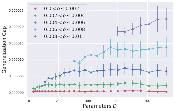
Figure 3 plots the generalization gap for different choices of δ\delta and D.D. The displayed generalization gap is the mean value over the repetitions. The error bars visualize the standard deviations. The plot shows empirically that the generalization gap is primarily influenced by the radius δ.\delta. Consistent with our theory, smaller values of δ\delta lead to more implicit regularization and therefore to a decrease in the generalization gap. On the contrary, the number of parameters DD only plays a minor role. Interestingly, for every δ\delta there is a regime where the generalization gap increases with the number of parameters until some saturation is attained. Beyond this regime, the number of parameters appears to have hardly any influence on the generalization gap.

Figure 4 shows how δ\delta and the width hh (recall that h=O⁡(D)h=O(\sqrt{D})) influence the stagnation probability. In line with the theoretical bounds, the stagnation probability increases as δ\delta get larger. The plot shows moreover, that the stagnation probability can get close to one and that a larger network width hh decreases the stagnation probability.
Refer to caption
Fig. 3: Dependence of the generalization gap on the number of parameters DD and δ\delta.
Refer to caption
Fig. 4: Stagnation probabilities in the population minima ℬδ​(μ)\mathcal{B}_{\delta}(\mu) for different choices of δ\delta and hh.

VI Conclusion

This work is a first attempt to describe the generalization error of deep learning under implicit regularization induced by the local shape of the loss surface. Previous work on implicit regularization focuses on norm bounds of the weight matrices. Instead we argue that the shape of the local minima for complex loss surfaces constraint later Gaussian SGD iterations resulting in improved bounds for the generalization gap. Implicit regularization through the shape of local minima is in line with the two phases of global and local search in SGD updates, also called the two-regime [70]. This is also reflected in the lower bound on the stagnation probability as it depends on the reaching probability and the non-escaping probability. The switch between reaching and non-escaping of local minima is driven by the decay of the learning rate.

We view this work as a very first step to explore loss surfaced based implicit regularization and hope that the presented ideas spark further research into this direction. We want to stress that in many respects, the obtained results in this work are preliminary. While we argue that the imposed conditions are natural for deep neural networks and also occur in related work, verifying them is an extremely hard problem beyond the scope of this work. Also it is clear that much tighter lower bounds for the staying probability should be obtainable. Finally, while we obtain bounds that do not directly depend on the number of neural network parameters, it remains unclear to which extend this dependence reoccurs through other quantities in these bounds.

VII Proof of Theorem 4

As already mentioned before, we need to lower bound the reaching probability and the non-escaping probability from 𝔅K,δ\mathfrak{B}_{K,\delta}. Let CΘ:=sup𝒜∈Θ‖𝒜‖FC_{\Theta}:=\sup_{\mathcal{A}\in\Theta}\|\mathcal{A}\|_{F}. For a subset ℬ⊂Θ\mathcal{B}\subset\Theta and a parameter 𝒜′∈Θ\mathcal{A}^{\prime}\in\Theta, ℬ+𝒜′:={𝒜+𝒜′∈Θ∣𝒜∈ℬ}\mathcal{B}+\mathcal{A}^{\prime}:=\{\mathcal{A}+\mathcal{A}^{\prime}\in\Theta\mid\mathcal{A}\in\mathcal{B}\} denotes the shifted set. We recall that if the updated parameter leaves Θ\Theta, it is projected back onto Θ\Theta. However, since the proofs in this section do not depend on the location of parameters in Θ\Theta and ℬδ​(μ)\mathcal{B}_{\delta}(\mu) does by construction not overlap with the boundary Θ\Theta, this projection does not affect the result.

VII-A Reaching Probability

We derive a lower bound for the reaching probability ℙ⁡(𝒜t¯∈𝔅K,δ)\mathbb{P}(\mathcal{A}_{\overline{t}}\in\mathfrak{B}_{K,\delta}) at time t¯\bar{t} as displayed in (4).

Theorem 9 (Reaching Probability).

Suppose Assumptions 1, 2, and 3 hold. Consider a monotonically decreasing learning rate ηt≍t−α\eta_{t}\asymp t^{-\alpha} with α>0\alpha>0 and let t¯\underline{t} be the first iteration tt such that t≥Cm,D,L,h¯,G,δ,𝔅t\geq C_{m,D,L,\bar{h},G,\delta,\mathfrak{B}} and ηt≤\eta_{t}\leq min{Cμ,R,∇R/(Lh¯2δ2),\min\{C_{\mu,R,\nabla R}/({L}\bar{h}^{2}\delta^{2}), Cξ,μn1/2/(L2δ2h¯4log(h¯D))}C_{\xi,\mu}n^{1/2}/(L^{2}\delta^{2}\bar{h}^{4}\log(\bar{h}D))\}. Suppose moreover that nn is sufficiently large such that n/log⁡n≥(ηt¯+1)2​(β0+1)​C2​ξ2​d/(β​δ)2n/\log n\geq(\eta_{\underline{t}}+1)^{2(\beta_{0}+1)}C^{2}\xi^{2}d/(\beta\delta)^{2}, and δ>Cm,L,h¯,D,G,Θ\delta>C_{m,L,\bar{h},D,G,\Theta} hold. Then, for any ε>0\varepsilon>0 and any t¯\bar{t} such that t¯−t¯≥C∗​(−t¯2​α​Cm,L,h¯,D,δ,G,Θ−log⁡(Cm,D,G​λ​(𝔅K,δ))𝐶𝐿𝑂𝑆𝐸\bar{t}-\underline{t}\geq C_{*}(-\bar{t}^{2\alpha}C_{m,L,\bar{h},D,\delta,G,\Theta}-\log(C_{m,D,G}\lambda(\mathfrak{B}_{K,\delta})), we obtain

ℙ⁡(𝒜t¯∈𝔅K,δ)\displaystyle\mathbb{P}(\mathcal{A}_{\bar{t}}\in\mathfrak{B}_{K,\delta}) ≥1−exp⁡(−Cm,L,h¯,D,δ,G,Θ​t¯2​α)Cm,D,G​λ​(𝔅K,δ).\displaystyle\geq 1-\frac{\exp\big(-C_{m,L,\bar{h},D,\delta,G,\Theta}\bar{t}^{2\alpha}\big)}{C_{m,D,G}\lambda(\mathfrak{B}_{K,\delta})}.
Proof.

Define the conditional probabilities pt:=ℙ⁡(𝒜t∈𝔅K,δ∣𝒜t−1∉𝔅K,δ)p_{t}:=\mathbb{P}(\mathcal{A}_{{t}}\in\mathfrak{B}_{K,\delta}\mid\mathcal{A}_{{t}-1}\notin\mathfrak{B}_{K,\delta}) and qt:=ℙ⁡(𝒜t∉𝔅K,δ∣𝒜t−1∈𝔅K,δ).q_{t}:=\mathbb{P}(\mathcal{A}_{{t}}\notin\mathfrak{B}_{K,\delta}\mid\mathcal{A}_{{t}-1}\in\mathfrak{B}_{K,\delta}). By Lemma 12 and Lemma 13, a sufficient large tt such that t≥max⁡{(CD,L,h¯,G​δ2/log⁡2),Cm,D,G′/log⁡(2​λ​(𝔅δ,K​Cm,G))}1/2​αt\geq\max\{(C_{D,L,\bar{h},G}\delta^{2}/\log 2),C^{\prime}_{m,D,G}/\log(2\lambda(\mathfrak{B}_{\delta,K}C_{m,G}))\}^{1/2\alpha} implies pt≤1/2p_{t}\leq 1/2 and qt≤1/2q_{t}\leq 1/2, hence we have pt+qt≤1p_{t}+q_{t}\leq 1.

These are the probabilities of entering or exiting the set 𝔅K,δ\mathfrak{B}_{K,\delta}. By the Markov property of the Gaussian SGD update, we have

ℙ⁡(𝒜t∈𝔅K,δ)\displaystyle\mathbb{P}(\mathcal{A}_{{t}}\in\mathfrak{B}_{K,\delta})
=(1−qt)​ℙ​(𝒜t−1∈𝔅K,δ)+pt​ℙ​(𝒜t−1∉𝔅K,δ),\displaystyle=(1-q_{t})\mathbb{P}(\mathcal{A}_{{t}-1}\in\mathfrak{B}_{K,\delta})+p_{t}\mathbb{P}(\mathcal{A}_{{t}-1}\notin\mathfrak{B}_{K,\delta}), (10)

and

ℙ⁡(𝒜t∉𝔅K,δ)\displaystyle\mathbb{P}(\mathcal{A}_{{t}}\notin\mathfrak{B}_{K,\delta})
=qt​ℙ​(𝒜t−1∉𝔅K,δ)+(1−pt)​ℙ​(𝒜t−1∈𝔅K,δ).\displaystyle=q_{t}\mathbb{P}(\mathcal{A}_{{t}-1}\notin\mathfrak{B}_{K,\delta})+(1-p_{t})\mathbb{P}(\mathcal{A}_{{t}-1}\in\mathfrak{B}_{K,\delta}). (11)

We now study the ratio

rt:=ℙ⁡(𝒜t∈𝔅K,δ)ℙ⁡(𝒜t∉𝔅K,δ)=ℙ⁡(𝒜t∈𝔅K,δ)1−ℙ⁡(𝒜t∈𝔅K,δ)∈(0,∞).\displaystyle r_{t}:=\frac{\mathbb{P}(\mathcal{A}_{{t}}\in\mathfrak{B}_{K,\delta})}{\mathbb{P}(\mathcal{A}_{{t}}\notin\mathfrak{B}_{K,\delta})}=\frac{\mathbb{P}(\mathcal{A}_{{t}}\in\mathfrak{B}_{K,\delta})}{1-\mathbb{P}(\mathcal{A}_{{t}}\in\mathfrak{B}_{K,\delta})}\in(0,\infty). (12)

Since the map (0,1)∋z↦z/(1−z)∈(0,∞)(0,1)\ni z\mapsto z/(1-z)\in(0,\infty) is bijective, there is an one-to-one correspondence between rtr_{t} and ℙ⁡(𝒜t∈𝔅K,δ)\mathbb{P}(\mathcal{A}_{{t}}\in\mathfrak{B}_{K,\delta}). Using (10) and (11), rtr_{t} can be rewritten into the recursive form

rt\displaystyle r_{t} =(1−qt)​ℙ​(𝒜t−1∈𝔅K,δ)+pt​(1−ℙ⁡(𝒜t−1∉𝔅K,δ))qt​ℙ​(𝒜t−1∈𝔅K,δ)+(1−pt)​(1−ℙ⁡(𝒜t−1∉𝔅K,δ))\displaystyle=\frac{(1-q_{t})\mathbb{P}(\mathcal{A}_{{t-1}}\in\mathfrak{B}_{K,\delta})+p_{t}(1-\mathbb{P}(\mathcal{A}_{{t-1}}\notin\mathfrak{B}_{K,\delta}))}{q_{t}\mathbb{P}(\mathcal{A}_{{t-1}}\in\mathfrak{B}_{K,\delta})+(1-p_{t})(1-\mathbb{P}(\mathcal{A}_{{t-1}}\notin\mathfrak{B}_{K,\delta}))}
=(1−qt)​rt−1+ptqt​rt−1+1−pt=:F⁡(rt−1,pt,qt).\displaystyle=\frac{(1-q_{t})r_{t-1}+p_{t}}{q_{t}r_{t-1}+1-p_{t}}=:F(r_{t-1};p_{t},q_{t}).

Based on this recursion, we now derive a lower bound for rt¯.r_{\bar{t}}. By Lemma 10, we obtain for 1≤t¯<t¯,1\leq\underline{t}<\bar{t},

rt¯≥mint∈[t¯,t¯]⁡ptqt−C​(1−c¯)t¯−t¯+1,\displaystyle r_{\bar{t}}\geq\min_{t\in[\underline{t},\overline{t}]}\frac{p_{t}}{q_{t}}-C(1-\bar{c})^{\bar{t}-\underline{t}+1}, (13)

for some c¯∈(0,1)\bar{c}\in(0,1). Applying the bounds for ptp_{t} and qtq_{t} in Proposition 11 and (19), it follows that

ptqt\displaystyle\frac{p_{{t}}}{q_{{t}}} ≥Cm,D,G​λ​(𝔅K,δ)​exp⁡(−Cm,G,Θ​ηt−2)CG​exp⁡(−Cm,L,h¯,D​δ2​ηt−2)\displaystyle\geq\frac{C_{m,D,G}\lambda(\mathfrak{B}_{K,\delta})\exp(-C_{m,G,\Theta}{\eta}_{t}^{-2})}{C_{G}\exp(-C_{m,L,\bar{h},D}\delta^{2}{\eta}_{t}^{-2})}
=exp⁡(t2​α​(Cm,L,h¯,D​δ2−Cm,G,Θ)CLOSE\displaystyle=\exp\Big(t^{2\alpha}(C_{m,L,\bar{h},D}\delta^{2}-C_{m,G,\Theta})
OPEN+log⁡(Cm,D,G​λ​(𝔅K,δ))),\displaystyle\qquad\qquad+\log(C_{m,D,G}\lambda(\mathfrak{B}_{K,\delta}))\Big), (14)

for every t≥t¯t\geq\underline{t}. By the definition (12) of rtr_{t}, as well as (13) and (14),

ℙ⁡(𝒜t¯∈𝔅K,δ)\displaystyle\mathbb{P}(\mathcal{A}_{\bar{t}}\in\mathfrak{B}_{K,\delta}) =rt¯1+rt¯\displaystyle=\frac{r_{\bar{t}}}{1+r_{\bar{t}}}
≥1−1rt¯\displaystyle\geq 1-\frac{1}{r_{\bar{t}}}
≥1−{exp(t¯2​α(Cm,L,h¯,Dδ2−Cm,G,Θ)\displaystyle\geq 1-\left\{\exp(\bar{t}^{2\alpha}(C_{m,L,\bar{h},D}\delta^{2}-C_{m,G,\Theta})\right.
+log(Cm,D,Gλ(𝔅K,δ)))−C(1−c¯)t¯−t¯}−1\displaystyle\qquad\left.+\log(C_{m,D,G}\lambda(\mathfrak{B}_{K,\delta})))-C(1-\bar{c})^{\bar{t}-\underline{t}}\right\}^{-1}

The lower bound for t¯−t¯\bar{t}-\underline{t}, entails the inequality 2−1​exp⁡(t¯2​α​(Cm,L,h¯,D​δ2−Cm,G,Θ)+log⁡(Cm,D,G​λ​(𝔅K,δ)))≥C​(1−c¯)t¯−t¯2^{-1}\exp(\bar{t}^{2\alpha}(C_{m,L,\bar{h},D}\delta^{2}-C_{m,G,\Theta})+\log(C_{m,D,G}\lambda(\mathfrak{B}_{K,\delta})))\geq C(1-\bar{c})^{\bar{t}-\underline{t}} proving

ℙ⁡(𝒜t¯∈𝔅K,δ)\displaystyle\mathbb{P}(\mathcal{A}_{\bar{t}}\in\mathfrak{B}_{K,\delta})
≥1−12​exp⁡(−t¯2​α​(Cm,L,h¯,D​δ2−Cm,G,Θ)CLOSE\displaystyle\geq 1-\frac{1}{2}\exp\Big(-\bar{t}^{2\alpha}(C_{m,L,\bar{h},D}\delta^{2}-C_{m,G,\Theta})
OPEN−log⁡(Cm,D,G​λ​(𝔅K,δ))).\displaystyle\qquad\qquad\qquad-\log\big(C_{m,D,G}\lambda(\mathfrak{B}_{K,\delta})\big)\Big).

Using the condition δ2>Cm,G,Θ/Cm,L,h¯,D\delta^{2}>C_{m,G,\Theta}/C_{m,L,\bar{h},D} and adjusting the constants, we obtain the statement. ∎

Lemma 10.

Suppose that there exists c¯>0\bar{c}>0 such that pt,qt∈[c¯,1−c¯]p_{t},q_{t}\in[\bar{c},1-\bar{c}] and pt+2​qt≤1p_{t}+2q_{t}\leq 1 for all t∈[t′,T]t\in[t^{\prime},T] with some t′≥1t^{\prime}\geq 1. For a positive sequence (rt)t(r_{t})_{t} defined as in (12), we have

rt¯≥mint∈[t¯,t¯]⁡ptqt−C​(1−c¯)t¯−t¯+1,\displaystyle r_{\bar{t}}\geq\min_{t\in[\underline{t},\overline{t}]}\frac{p_{t}}{q_{t}}-C(1-\bar{c})^{\bar{t}-\underline{t}+1},

for some positive constant CC.

Proof.

We use that F(⋅;pt,qt)=((1−qt)⋅+pt)/(qt⋅+1−pt)F(\cdot;p_{t},q_{t})=((1-q_{t})\cdot+p_{t})/(q_{t}\cdot+1-p_{t}) is a contraction and show that rtr_{t} gets close to a fixed point of F⁡(⋅,pt,qt)F(\cdot;p_{t},q_{t}) as tt increases.

To prove this, we need several elementary properties of F⁡(⋅,pt,qt).F(\cdot;p_{t},q_{t}). Since ∂r′F⁡(r′,pt,qt)=(1−pt−qt)/(1−pt+qt​r′)2\partial_{r^{\prime}}F(r^{\prime};p_{t},q_{t})=(1-p_{t}-q_{t})/(1-p_{t}+q_{t}r^{\prime})^{2}, F⁡(r′,pt,qt)F(r^{\prime};p_{t},q_{t}) is monotonically increasing in r′r^{\prime} whenever pt+qt≤1p_{t}+q_{t}\leq 1. Also, F⁡(r′,pt,qt)F(r^{\prime};p_{t},q_{t}) is strictly concave in r′r^{\prime} since ∂r′2F⁡(r′,pt,qt)<0\partial_{r^{\prime}}^{2}F(r^{\prime};p_{t},q_{t})<0 holds. Moreover, we have F⁡(0,pt,qt)=pt/(1−pt)>0F(0;p_{t},q_{t})=p_{t}/(1-p_{t})>0.

Using these properties, for each tt, there exists a unique fixed point rt∗r_{t}^{*} satisfying

rt∗=F⁡(rt∗,pt,qt).\displaystyle r_{t}^{*}=F(r_{t}^{*};p_{t},q_{t}).

Since pt/qtp_{t}/q_{t} is a fixed point, we must have rt∗=pt/qtr_{t}^{*}=p_{t}/q_{t}. We show that rt∗r_{t}^{*} is an attractor. That is, for r∈(0,∞)r\in(0,\infty), we have

|F⁡(r,pt,qt)−F⁡(rt∗,pt,qt)|\displaystyle|F(r;p_{t},q_{t})-F(r_{t}^{*};p_{t},q_{t})| =|1−qt​(1+r)1+qt​r−pt|​|r−rt∗|\displaystyle=\Big|1-\frac{q_{t}(1+r)}{1+q_{t}r-p_{t}}\Big||r-r_{t}^{*}|
≤(1−c¯)​|r−rt∗|,\displaystyle\leq(1-\bar{c})|r-r_{t}^{*}|, (15)

where the last inequality follows from the fact that qt​(1+r)>c¯q_{t}(1+r)>\bar{c} implies 1−qt​(1+r)1+qt​r−pt≤1−c¯1-\frac{q_{t}(1+r)}{1+q_{t}r-p_{t}}\leq 1-\bar{c}, and qt+(2−c¯)​pt<2−c¯q_{t}+(2-\bar{c})p_{t}<2-\bar{c} implies qt​(1+r)1+qt​r−pt−1≤1−c¯\frac{q_{t}(1+r)}{1+q_{t}r-p_{t}}-1\leq 1-\bar{c}. The first condition qt​(1+r)>c¯q_{t}(1+r)>\bar{c} is implied by qt≥c¯q_{t}\geq\bar{c}, and the second condition qt+(2−c¯)​pt<2−c¯q_{t}+(2-\bar{c})p_{t}<2-\bar{c} follows from pt+2​qt≤1p_{t}+2q_{t}\leq 1.

Due to the concavity of F⁡(⋅,pt,qt)F(\cdot;p_{t},q_{t}), we know that r≥F⁡(r,pt,qt)≥rt∗r\geq F(r;p_{t},q_{t})\geq r_{t}^{*} holds if and only if r<rt∗r<r_{t}^{*}, and r≤F⁡(r,pt,qt)≤rt∗r\leq F(r;p_{t},q_{t})\leq r_{t}^{*} holds if and only if r>rt∗r>r_{t}^{*}.

For any t∈[t¯,t¯]t\in[\underline{t},\bar{t}], we derive now a lower bound for rt¯−mint⁡rt∗r_{\bar{t}}-\min_{t}r_{{t}}^{*}. We treat two cases, depending on whether the sequence (rt)t∈[t¯,t¯](r_{t})_{t\in[\underline{t},\overline{t}]} is increasing or not. If (rt)t∈[t¯,t¯](r_{t})_{t\in[\underline{t},\overline{t}]} is not an increasing sequence, there exists t′∈[t¯,t¯−t]t^{\prime}\in[\underline{t},\overline{t}-t] such that rt′+1≤rt′r_{t^{\prime}+1}\leq r_{t^{\prime}}. By the property of F⁡(⋅,pt,qt)F(\cdot;p_{t},q_{t}) derived above, this implies rt′≥rt′∗r_{t^{\prime}}\geq r_{t^{\prime}}^{*}. Because of rt′∗≥mint⁡rt∗r_{t^{\prime}}^{*}\geq\min_{t}r_{{t}}^{*}, we know that for any τ∈[1,t¯−t′]\tau\in[1,\bar{t}-t^{\prime}] the value rt′+τr_{t^{\prime}+\tau} cannot be larger than mint∈[t¯,t¯]⁡rt∗\min_{t\in[\underline{t},\overline{t}]}r_{t}^{*}. Thus rt¯−mint∈[t¯,t¯]⁡rt∗≥0r_{\bar{t}}-\min_{t\in[\underline{t},\overline{t}]}r_{{t}}^{*}\geq 0.

We now consider the second case assuming that (rt)t∈[t¯,t¯](r_{t})_{t\in[\underline{t},\overline{t}]} is an increasing sequence, that is, rt≤rt+1r_{t}\leq r_{t+1} for all t∈[t¯,t¯−1]t\in[\underline{t},\overline{t}-1]. Without loss of generality, we can moreover assume that maxt∈[t¯,t¯]⁡rt≤mint∈[t¯,t¯]⁡rt∗\max_{t\in[\underline{t},\overline{t}]}r_{t}\leq\min_{t\in[\underline{t},\overline{t}]}r_{t}^{*} since otherwise, by the monotone increase of (rt)t(r_{t})_{t}, rt¯=maxt∈[t¯,t¯]⁡rt≥mint∈[t¯,t¯]⁡rt∗=mint∈[t¯,t¯]⁡pt/qtr_{\bar{t}}=\max_{t\in[\underline{t},\overline{t}]}r_{t}\geq\min_{t\in[\underline{t},\overline{t}]}r_{t}^{*}=\min_{t\in[\underline{t},\overline{t}]}p_{t}/q_{t} automatically implies the statement of Lemma 10. Observe that z↦(z−rt′)/(z−rt′−1)z\mapsto(z-r_{t^{\prime}})/(z-r_{t^{\prime}-1}) is an increasing function due to rt′≥rt′−1.r_{t^{\prime}}\geq r_{t^{\prime}-1}. Together with (15) this gives

mint∈[t¯,t¯]⁡rt∗−rt¯\displaystyle\min_{t\in[\underline{t},\overline{t}]}r_{t}^{*}-r_{\bar{t}} =(mint∈[t¯,t¯]⁡rt∗−rt¯)​∏t′=t¯+1t¯mint∈[t¯,t¯]⁡rt∗−rt′mint∈[t¯,t¯]⁡rt∗−rt′−1\displaystyle=\left(\min_{t\in[\underline{t},\overline{t}]}r_{t}^{*}-r_{\underline{t}}\right)\prod_{t^{\prime}=\underline{t}+1}^{\bar{t}}\frac{\min_{t\in[\underline{t},\overline{t}]}r_{t}^{*}-r_{t^{\prime}}}{\min_{t\in[\underline{t},\overline{t}]}r_{t}^{*}-r_{t^{\prime}-1}}
≤(mint∈[t¯,t¯]⁡rt∗−rt¯)​∏t′=t¯+1t¯rt′∗−rt′rt′∗−rt′−1\displaystyle\leq\left(\min_{t\in[\underline{t},\overline{t}]}r_{t}^{*}-r_{\underline{t}}\right)\prod_{t^{\prime}=\underline{t}+1}^{\bar{t}}\frac{r_{t^{\prime}}^{*}-r_{t^{\prime}}}{r_{t^{\prime}}^{*}-r_{t^{\prime}-1}}
≤(mint∈[t¯,t¯]⁡rt∗−rt¯)​(1−c¯)t¯−t¯.\displaystyle\leq\left(\min_{t\in[\underline{t},\overline{t}]}r_{t}^{*}-r_{\underline{t}}\right)(1-\bar{c})^{\bar{t}-\underline{t}}.

Combining both cases, we obtain that

rt¯\displaystyle r_{\bar{t}} ≥mint∈[t¯,t¯]⁡rt∗−(mint∈[t¯,t¯]⁡rt∗−rt¯)​(1−c¯)t¯−t¯\displaystyle\geq\min_{t\in[\underline{t},\overline{t}]}r_{t}^{*}-\left(\min_{t\in[\underline{t},\overline{t}]}r_{t}^{*}-r_{\underline{t}}\right)(1-\bar{c})^{\bar{t}-\underline{t}}
≥mint∈[t¯,t¯]⁡rt∗−(mint∈[t¯,t¯]⁡rt∗)​(1−c¯)t¯−t¯\displaystyle\geq\min_{t\in[\underline{t},\overline{t}]}r_{t}^{*}-\left(\min_{t\in[\underline{t},\overline{t}]}r_{t}^{*}\right)(1-\bar{c})^{\bar{t}-\underline{t}}
≥mint∈[t¯,t¯]⁡rt∗−Cc¯​(1−c¯)t¯−t¯+1,\displaystyle\geq\min_{t\in[\underline{t},\overline{t}]}r_{t}^{*}-C_{\bar{c}}(1-\bar{c})^{\bar{t}-\underline{t}+1},

Together with the definition rt∗=pt/qtr_{t}^{*}=p_{t}/q_{t}, we obtain the result. ∎

Proposition 11.

Consider Gaussian SGD as defined in Section II-C. For any 𝒜t∈Θ\mathcal{A}_{t}\in\Theta and any learning rate ηt≍t−2​α\eta_{t}\asymp t^{-2\alpha} with ηt≤1\eta_{t}\leq 1 for all tt, we obtain

ℙ⁡(𝒜t+1∈𝔅K,δ∣𝒜t)≥λ⁡(𝔅K,δ)​Cm,D,G​exp⁡(−Cm,G,Θ​t2​α).\displaystyle\mathbb{P}(\mathcal{A}_{t+1}\in\mathfrak{B}_{K,\delta}\mid\mathcal{A}_{t})\geq\lambda(\mathfrak{B}_{K,\delta})C_{m,D,G}\exp\left(-C_{m,G,\Theta}t^{2\alpha}\right).
Proof.

We set U~t+1:=m−1/2ηtUt+1(𝒜t)∼𝒩(0,ηt2G(𝒜t)/m),\tilde{U}_{t+1}:=m^{-1/2}{\eta_{t}}U_{t+1}(\mathcal{A}_{t})\sim\mathcal{N}(0,\eta_{t}^{2}G(\mathcal{A}_{t})/m), and define the event ℰt+1:={U~t+1∈𝔅K,δ−𝒜t+ηt∇Rn(𝒜t)}.\mathcal{E}_{t+1}:=\{\tilde{U}_{t+1}\in\mathfrak{B}_{K,\delta}-\mathcal{A}_{t}+\eta_{t}\nabla R_{n}(\mathcal{A}_{t})\}. By assumption, all eigenvalues of the covariance matrix G⁡(𝒜t)G(\mathcal{A}_{t}) lie in the interval [cG′,cG][c_{G}^{\prime},c_{G}] with cG′>0.c_{G}^{\prime}>0. Recall that λ⁡(ℬ)\lambda(\mathcal{B}) denotes the Lebesgue measure of the set ℬ\mathcal{B} and that the Lebesgue measure is invariant under location shifts. Therefore

ℙU~t+1|𝒜t​(ℰt+1)\displaystyle\mathbb{P}_{\tilde{U}_{t+1}|\mathcal{A}_{t}}({\mathcal{E}}_{t+1})
=∫𝔅K,δ−𝒜t+ηt∇Rn(𝒜t)dℙU~t+1|𝒜t(u)\displaystyle=\int_{\mathfrak{B}_{K,\delta}-\mathcal{A}_{t}+\eta_{t}\nabla R_{n}(\mathcal{A}_{t})}d\mathbb{P}_{\tilde{U}_{t+1}|\mathcal{A}_{t}}(u)
≥λ(𝔅K,δ−𝒜t+ηt∇Rn(𝒜t))\displaystyle\geq\lambda\big(\mathfrak{B}_{K,\delta}-\mathcal{A}_{t}+\eta_{t}\nabla R_{n}(\mathcal{A}_{t})\big)
infu∈𝔅K,δ−𝒜t+ηt∇Rn(𝒜t)d​ℙU~t+1|𝒜td​λ(u)\displaystyle\quad\inf_{u\in\mathfrak{B}_{K,\delta}-\mathcal{A}_{t}+\eta_{t}\nabla R_{n}(\mathcal{A}_{t})}\frac{d\mathbb{P}_{\tilde{U}_{t+1}|\mathcal{A}_{t}}}{d\lambda}(u)
≥λ(𝔅K,δ)infu∈𝔅K,δ−𝒜t+ηt∇Rn(𝒜t)1(2​π)D​|ηt2m​G​(𝒜t)|\displaystyle\geq\lambda(\mathfrak{B}_{K,\delta})\inf_{u\in\mathfrak{B}_{K,\delta}-\mathcal{A}_{t}+\eta_{t}\nabla R_{n}(\mathcal{A}_{t})}\frac{1}{\sqrt{(2\pi)^{D}|\frac{\eta_{t}^{2}}{m}G(\mathcal{A}_{t})|}}
×exp⁡(−m2​ηt2​vec​(u)⊤​(G⁡(𝒜t))−1​vec​(u))\displaystyle\quad\times\exp\left(-\frac{m}{2\eta_{t}^{2}}\mathrm{vec}(u)^{\top}(G(\mathcal{A}_{t}))^{-1}\mathrm{vec}(u)\right)
≳λ⁡(𝔅K,δ)(2​π​ηt2/m)D/2​|G⁡(𝒜t)|1/2​exp⁡(−m2​ηt2​cG′​CΘ2)\displaystyle\gtrsim\frac{\lambda(\mathfrak{B}_{K,\delta})}{{(2\pi\eta_{t}^{2}/m)^{D/2}|G(\mathcal{A}_{t})|^{1/2}}}\exp\left(-\frac{m}{2\eta_{t}^{2}c_{G}^{\prime}}C_{\Theta}^{2}\right)
≥λ⁡(𝔅K,δ)(2​π/m)D/2​|G⁡(𝒜t)|1/2​exp⁡(−m2​ηt2​cG′​CΘ2),\displaystyle\geq\frac{\lambda(\mathfrak{B}_{K,\delta})}{{(2\pi/m)^{D/2}|G(\mathcal{A}_{t})|^{1/2}}}\exp\left(-\frac{m}{2\eta_{t}^{2}c_{G}^{\prime}}C_{\Theta}^{2}\right),

where the second to last inequality follows from ‖u‖22≤max𝒜∈Θ⁡‖𝒜‖F2=CΘ2\|u\|_{2}^{2}\leq\max_{\mathcal{A}\in\Theta}\|\mathcal{A}\|_{F}^{2}=C_{\Theta}^{2} and vec​(u)⊤​(G⁡(𝒜t))−1​vec​(u)≤‖u‖22/cG′≤CΘ2/cG′\mathrm{vec}(u)^{\top}(G(\mathcal{A}_{t}))^{-1}\newline \mathrm{vec}(u)\leq\|u\|_{2}^{2}/c_{G}^{\prime}\leq C_{\Theta}^{2}/c_{G}^{\prime} for any 𝒜∈𝔅K,δ\mathcal{A}\in\mathfrak{B}_{K,\delta}, and in the last step we applied ηt≤1\eta_{t}\leq 1 for any tt.

Since c​t−α≤ηtct^{-\alpha}\leq\eta_{t}, we obtain the statement with Cm,D,G=(2πcG2/m)−D/2C_{m,D,G}=(2\pi c_{G}^{2}/m)^{-D/2} and Cm,G,Θ=m​CΘ2/(c​cG′)2C_{m,G,\Theta}=mC_{\Theta}^{2}/(cc_{G}^{\prime})^{2}. ∎

Lemma 12.

Consider Gaussian SGD as defined in Section II-C. For any 𝒜t∈Θ\mathcal{A}_{t}\in\Theta and any learning rate ηt≍t−2​α\eta_{t}\asymp t^{-2\alpha} with ηt≤1\eta_{t}\leq 1 for all tt, we obtain

ℙ⁡(𝒜t+1∈𝔅K,δ∣𝒜t∉𝔅K,δ)\displaystyle\mathbb{P}(\mathcal{A}_{t+1}\in\mathfrak{B}_{K,\delta}\mid\mathcal{A}_{t}\notin\mathfrak{B}_{K,\delta})
≤λ⁡(𝔅K,δ)​Cm,D,G′​exp⁡(−Cm,G​t2​α).\displaystyle\leq\lambda(\mathfrak{B}_{K,\delta})C^{\prime}_{m,D,G}\exp\left(-C_{m,G}t^{2\alpha}\right).
Proof.

Similar to the proof of Proposition 11, we set U~t+1:=m−1/2ηtUt+1(𝒜t)∼𝒩(0,ηt2G(𝒜t)/m),\tilde{U}_{t+1}:=m^{-1/2}{\eta_{t}}U_{t+1}(\mathcal{A}_{t})\sim\mathcal{N}(0,\eta_{t}^{2}G(\mathcal{A}_{t})/m), and ℰt+1:={U~t+1∈𝔅K,δ−𝒜t+ηt∇Rn(𝒜t)}.\mathcal{E}_{t+1}:=\{\tilde{U}_{t+1}\in\mathfrak{B}_{K,\delta}-\mathcal{A}_{t}+\eta_{t}\nabla R_{n}(\mathcal{A}_{t})\}. Define Δt=min𝒜∈𝔅K,δ⁡‖𝒜t−𝒜‖F>0\Delta_{t}=\min_{\mathcal{A}\in\mathfrak{B}_{K,\delta}}\|\mathcal{A}_{t}-\mathcal{A}\|_{F}>0. We derive the following upper bound

ℙU~t+1|𝒜t∉𝔅K,δ​(ℰt+1)\displaystyle\mathbb{P}_{\tilde{U}_{t+1}|\mathcal{A}_{t}\notin\mathfrak{B}_{K,\delta}}({\mathcal{E}}_{t+1})
≤λ(𝔅K,δ−𝒜t+ηt∇Rn(𝒜t))\displaystyle\leq\lambda\big(\mathfrak{B}_{K,\delta}-\mathcal{A}_{t}+\eta_{t}\nabla R_{n}(\mathcal{A}_{t})\big)
maxu∈𝔅K,δ−𝒜t+ηt∇Rn(𝒜t)d​ℙU~t+1|𝒜t∉𝔅K,δd​λ(u)\displaystyle\quad\max_{u\in\mathfrak{B}_{K,\delta}-\mathcal{A}_{t}+\eta_{t}\nabla R_{n}(\mathcal{A}_{t})}\frac{d\mathbb{P}_{\tilde{U}_{t+1}|\mathcal{A}_{t}\notin\mathfrak{B}_{K,\delta}}}{d\lambda}(u)
=λ(𝔅K,δ)maxu∈𝔅K,δ−𝒜t+ηt∇Rn(𝒜t)1(2​π)D​|ηt2m​G​(𝒜t)|\displaystyle=\lambda(\mathfrak{B}_{K,\delta})\max_{u\in\mathfrak{B}_{K,\delta}-\mathcal{A}_{t}+\eta_{t}\nabla R_{n}(\mathcal{A}_{t})}\frac{1}{\sqrt{(2\pi)^{D}|\frac{\eta_{t}^{2}}{m}G(\mathcal{A}_{t})|}}
×exp⁡(−m2​ηt2​vec​(u)⊤​(G⁡(𝒜t))−1​vec​(u))\displaystyle\quad\times\exp\left(-\frac{m}{2\eta_{t}^{2}}\mathrm{vec}(u)^{\top}(G(\mathcal{A}_{t}))^{-1}\mathrm{vec}(u)\right)
≤λ⁡(𝔅K,δ)(2​π​ηt2/m)D/2​|G⁡(𝒜t)|1/2​exp⁡(−m2​ηt2​cG​Δt2),\displaystyle\leq\frac{\lambda(\mathfrak{B}_{K,\delta})}{{(2\pi\eta_{t}^{2}/m)^{D/2}|G(\mathcal{A}_{t})|^{1/2}}}\exp\left(-\frac{m}{2\eta_{t}^{2}c_{G}}\Delta_{t}^{2}\right),

where the last inequality follows from the bound on the eigenvalues of G⁡(𝒜t)G(\mathcal{A}_{t}) and the definition of Δt\Delta_{t}. Since c​t−α≤ηtct^{-\alpha}\leq\eta_{t}, we obtain the statement with Cm,D,G′=(2π(cG′)2/m)−D/2C^{\prime}_{m,D,G}=(2\pi(c^{\prime}_{G})^{2}/m)^{-D/2} and Cm,G=m​Δt2/(c​cG)2C_{m,G}=m\Delta_{t}^{2}/(cc_{G})^{2}. ∎

VII-B Non-escaping Probability

In this section, we derive a lower bound for ℙ(𝒜t∈𝔅K,δ,∀t≥τ∣τℬ=τ).\mathbb{P}(\mathcal{A}_{t}\in\mathfrak{B}_{K,\delta},\forall t\geq\tau\mid\tau_{\mathcal{B}}=\tau). As preparation, for time t¯>t¯≥0\overline{t}>\underline{t}\geq 0, constants c∈(0,1)c\in(0,1), c′>0c^{\prime}>0 and a parameter κ>0\kappa>0, we define

ζ⁡(t¯,t¯,c,c′,κ):=∏τ=t¯t¯(1−c​exp⁡(−c′​τκ)).\displaystyle\zeta(\underline{t},\overline{t},c,c^{\prime},\kappa):=\prod_{\tau=\underline{t}}^{\overline{t}}(1-c\exp(-c^{\prime}\tau^{\kappa})). (16)

Obviously, ζ⁡(t¯,t¯,c,c′,κ)∈(0,1)\zeta(\underline{t},\overline{t},c,c^{\prime},\kappa)\in(0,1) and ζ⁡(t¯,t¯,c,c′,κ)\zeta(\underline{t},\overline{t},c,c^{\prime},\kappa) increases in cc, and decreases in c′c^{\prime}.

Lemma 13 (Noise Gradient Lemma).

Suppose the parameter space Θ\Theta contains {0}\{0\}. Let 𝒜∈ℬδ​(μ)\mathcal{A}\in\mathcal{B}_{\delta}(\mu) be a parameter such that ε=‖𝒜−Πμ​(𝒜)‖L,2,1\varepsilon=\|\mathcal{A}-\Pi_{\mu}(\mathcal{A})\|_{L,2,1} with ε∈(0,δ)\varepsilon\in(0,\delta). For an ℝD\mathbb{R}^{D}-valued random variable W∼𝒩⁡(0,G⁡(𝒜))W\sim\mathcal{N}(0,G(\mathcal{A})) and δ∈(0,D)\delta\in(0,D), we obtain

ℙW​(𝒜+W∉ℬδ​(μ))≤exp⁡(−D​(δ−ε)2128​L​h¯​cG′).\displaystyle\mathbb{P}_{W}\left(\mathcal{A}+W\notin\mathcal{B}_{\delta}(\mu)\right)\leq\exp\left(-\frac{D(\delta-\varepsilon)^{2}}{128L\bar{h}c_{G}^{\prime}}\right).
Proof.

For any 𝒜′∈ℬδ−ε​({𝒜})\mathcal{A}^{\prime}\in\mathcal{B}_{\delta-\varepsilon}(\{\mathcal{A}\}), we have ‖𝒜′−Πμ​(𝒜)‖L,2,1≤‖𝒜′−𝒜‖L,2,1+‖𝒜−Πμ​(𝒜)‖L,2,1≤δ−ε+ε=δ\|\mathcal{A}^{\prime}-\Pi_{\mu}(\mathcal{A})\|_{L,2,1}\leq\|\mathcal{A}^{\prime}-\mathcal{A}\|_{L,2,1}+\|\mathcal{A}-\Pi_{\mu}(\mathcal{A})\|_{L,2,1}\leq\delta-\varepsilon+\varepsilon=\delta. This yields the inclusions

ℬδ−ε​({𝒜})⊂ℬδ​(Πμ​(𝒜))⊆ℬδ​(μ).\displaystyle\mathcal{B}_{\delta-\varepsilon}(\{\mathcal{A}\})\subset\mathcal{B}_{\delta}(\Pi_{\mu}(\mathcal{A}))\subseteq\mathcal{B}_{\delta}(\mu). (17)

We now bound the probability that 𝒜+W\mathcal{A}+W does not lie in ℬδ​(μ)\mathcal{B}_{\delta}(\mu) anymore. Here, we additionally consider a neighbourhood of {𝒜}\{\mathcal{A}\} in terms of the norm ‖𝒜‖F\|\mathcal{A}\|_{F}. Lemma 22 states that ‖𝒜‖L,2,1≤L​h¯​‖𝒜‖F.\|\mathcal{A}\|_{L,2,1}\leq\sqrt{L\bar{h}}\|\mathcal{A}\|_{F}. Thus,

ℙW​(𝒜+W∉ℬδ−ε​({𝒜}))\displaystyle\mathbb{P}_{W}\big(\mathcal{A}+W\notin\mathcal{B}_{\delta-\varepsilon}(\{\mathcal{A}\})\big)
≤ℙW​(𝒜+W∉{z:‖z−𝒜‖F≥(δ−ε)/L​h¯}).\displaystyle\leq\mathbb{P}_{W}\left(\mathcal{A}+W\notin\left\{z:\|z-\mathcal{A}\|_{F}\geq(\delta-\varepsilon)/\sqrt{L\bar{h}}\right\}\right).

By the Gaussianity of WW, we obtain

ℙW​(𝒜+W∉{z:‖z−𝒜‖F≥(δ−ε)/L​h¯})\displaystyle\mathbb{P}_{W}\left(\mathcal{A}+W\notin\left\{z:\|z-\mathcal{A}\|_{F}\geq(\delta-\varepsilon)/\sqrt{L\bar{h}}\right\}\right)
=ℙW​({z:‖z‖F≥(δ−ε)/L​h¯})\displaystyle=\mathbb{P}_{W}\left(\{z:\|z\|_{F}\geq(\delta-\varepsilon)/\sqrt{L\bar{h}}\}\right)
≤exp⁡(−D​(δ−ε)264​L​h¯​cz).\displaystyle\leq\exp\left(-\frac{D(\delta-\varepsilon)^{2}}{64L\bar{h}c_{z}}\right).

The last inequality follows from Proposition 1 in [79] and since, without loss of generality, we can assume δ<D.\delta<D. ∎

We derive now a lower bound for the non-escaping probability.

Theorem 14 (Non-Escaping Probability).

Work under the assumptions of Theorem 4. If 𝒜t¯∈ℬδ​(μ)\mathcal{A}_{\bar{t}}\in\mathcal{B}_{\delta}(\mu) holds at time t¯\bar{t}, then for any t>t¯t>\bar{t} such as ηt≤min{Cμ,R(C∇RLh¯δ)−2,\eta_{t}\leq\min\{C_{\mu,R}(C_{\nabla R}\sqrt{L}\bar{h}\delta)^{-2}, Cξ,μn1/2/(L2δ2h¯4log(h¯D))}C_{\xi,\mu}n^{1/2}/(L^{2}\delta^{2}\bar{h}^{4}\log(\bar{h}D))\} and all sufficiently large nn, we have

ℙ𝒜(𝒜τ∈ℬδ(μ),∀τ∈(t¯,t]∣𝒜t¯∈ℬδ(μ))\displaystyle\mathbb{P}_{\mathcal{A}}\left(\mathcal{A}_{\tau}\in\mathcal{B}_{\delta}(\mu),\forall\tau\in(\bar{t},t]\mid\mathcal{A}_{\bar{t}}\in\mathcal{B}_{\delta}(\mu)\right)
≥∏τ=t¯+1t{1−CG​exp⁡(−Cm,L,h¯,D​δ2​ητ−2)}.\displaystyle\geq\prod_{\tau=\bar{t}+1}^{t}\left\{1-C_{G}\exp\left(-C_{m,L,\bar{h},D}\delta^{2}\eta_{\tau}^{-2}\right)\right\}.
Proof.

For the tt-th iteration, we define the following event

ℰt:={𝒜t∈ℬδ(μ)}.\displaystyle\mathcal{E}_{t}:=\{\mathcal{A}_{t}\in\mathcal{B}_{\delta}(\mu)\}.

By the Markov property of the Gaussian SGD update rule (6), we have

ℙ𝒜(𝒜τ∈ℬδ(μ),∀τ∈(t¯,t]∣𝒜t¯∈ℬδ(μ))\displaystyle\mathbb{P}_{\mathcal{A}}\big(\mathcal{A}_{\tau}\in\mathcal{B}_{\delta}(\mu),\forall\tau\in(\bar{t},t]\mid\mathcal{A}_{\bar{t}}\in\mathcal{B}_{\delta}(\mu)\big)
=ℙ𝒜​(⋂τ=τ¯+1tℰτ∣ℰt¯)=∏τ=t¯+1tℙ𝒜​(ℰτ∣ℰτ−1).\displaystyle=\mathbb{P}_{\mathcal{A}}\left(\bigcap_{\tau=\bar{\tau}+1}^{t}\mathcal{E}_{\tau}\mid\mathcal{E}_{\bar{t}}\right)=\prod_{\tau=\bar{t}+1}^{t}\mathbb{P}_{\mathcal{A}}\left(\mathcal{E}_{\tau}\mid\mathcal{E}_{\tau-1}\right). (18)

We now evaluate the step-wise non-escaping probability ℙ𝒜​(ℰτ∣ℰτ−1)\mathbb{P}_{\mathcal{A}}\left(\mathcal{E}_{\tau}\mid\mathcal{E}_{\tau-1}\right) for τ≥t¯+1\tau\geq\bar{t}+1. In a first step, we consider the parameter update 𝒜τ−:=𝒜τ−1−ητ−1∇Rn(𝒜τ−1)\mathcal{A}_{\tau}^{-}:=\mathcal{A}_{\tau-1}-\eta_{\tau-1}\nabla R_{n}(\mathcal{A}_{\tau-1}) and study the probability that 𝒜τ−∈ℬδ​(μ)\mathcal{A}_{\tau}^{-}\in\mathcal{B}_{\delta}(\mu) holds. To this end, we consider the obvious inequality ‖𝒜τ−−Πμ​(𝒜τ−)‖L,2,1≤‖𝒜τ−−Πμ​(𝒜τ−1)‖L,2,1\|\mathcal{A}_{\tau}^{-}-\Pi_{\mu}(\mathcal{A}_{\tau}^{-})\|_{L,2,1}\leq\|\mathcal{A}_{\tau}^{-}-\Pi_{\mu}(\mathcal{A}_{\tau-1})\|_{L,2,1}. By Lemma 15, we obtain

‖𝒜τ−−Πμ​(𝒜τ−1)‖L,2,1<‖𝒜τ−1−Πμ​(𝒜τ−1)‖L,2,1,\displaystyle\|\mathcal{A}_{\tau}^{-}-\Pi_{\mu}(\mathcal{A}_{\tau-1})\|_{L,2,1}<\|\mathcal{A}_{\tau-1}-\Pi_{\mu}(\mathcal{A}_{\tau-1})\|_{L,2,1},

with probability at least 1−ε1-\varepsilon for the specified ητ−1\eta_{\tau-1} and nn. Setting ε=exp(−1/ητ−12)\varepsilon=\exp(-1/\eta_{\tau-1}^{2}) gives

‖𝒜τ−−Πμ​(𝒜τ−1−)‖L,2,1\displaystyle\|\mathcal{A}_{\tau}^{-}-\Pi_{\mu}(\mathcal{A}_{\tau-1}^{-})\|_{L,2,1} ≤‖𝒜τ−1−−Πμ​(𝒜τ−1)‖L,2,1\displaystyle\leq\|\mathcal{A}_{\tau-1}^{-}-\Pi_{\mu}(\mathcal{A}_{\tau-1})\|_{L,2,1}
≤‖𝒜τ−1−Πμ​(𝒜τ−1)‖L,2,1.\displaystyle\leq\|\mathcal{A}_{\tau-1}-\Pi_{\mu}(\mathcal{A}_{\tau-1})\|_{L,2,1}.

Hence, we have 𝒜τ−∈ℬδ​(μ)\mathcal{A}_{\tau}^{-}\in\mathcal{B}_{\delta}(\mu).

We apply Lemma 13 and evaluate ℙ𝒜​(ℰτ∣ℰτ−1)\mathbb{P}_{\mathcal{A}}\left(\mathcal{E}_{\tau}\mid\mathcal{E}_{\tau-1}\right). Replacing in the notation of Lemma 13 the parameter 𝒜\mathcal{A} by 𝒜τ−1\mathcal{A}_{\tau-1} and the gradient noise UU by ητm​Uτ​(𝒜τ−1)\frac{\eta_{\tau}}{\sqrt{m}}U_{\tau}(\mathcal{A}_{\tau-1}), we obtain

ℙ𝒜​(ℰτ∣ℰτ−1)\displaystyle\mathbb{P}_{\mathcal{A}}\left(\mathcal{E}_{\tau}\mid\mathcal{E}_{\tau-1}\right)
=ℙU​(𝒜+U∈ℬδ​(μ))\displaystyle=\mathbb{P}_{U}\left(\mathcal{A}+U\in\mathcal{B}_{\delta}(\mu)\right)
=1−ℙU​(𝒜+U∉ℬδ​(μ))−ε\displaystyle=1-\mathbb{P}_{U}(\mathcal{A}+U\notin\mathcal{B}_{\delta}(\mu))-\varepsilon
≥1−exp⁡(−C​D​m​δ2L​h¯​ητ2​cG′)​|m−1​ητ2​I||ΣU|−exp⁡(−1ητ2),\displaystyle\geq 1-\exp\left(-\frac{CDm\delta^{2}}{L\bar{h}\eta_{\tau}^{2}c_{G}^{\prime}}\right)\sqrt{\frac{|m^{-1}\eta_{\tau}^{2}I|}{|\Sigma_{U}|}}-\exp\left(-\frac{1}{\eta_{\tau}^{2}}\right),

where ΣU\Sigma_{U} is the covariance matrix of ητm​Uτ​(𝒜τ−1)\frac{\eta_{\tau}}{\sqrt{m}}U_{\tau}(\mathcal{A}_{\tau-1}), and CC is a universal constant. From that, we obtain

ℙ𝒜​(ℰτ∣ℰτ−1)≥1−CG​exp⁡(−Cm,L,h¯,D​δ2​ητ−2),\displaystyle\mathbb{P}_{\mathcal{A}}\left(\mathcal{E}_{\tau}\mid\mathcal{E}_{\tau-1}\right)\geq 1-C_{G}\exp\left(-C_{m,L,\bar{h},D}\delta^{2}\eta_{\tau}^{-2}\right), (19)

with CG=2​|m−1​ητ2​I||ΣU|=2​|I||G⁡(𝒜τ−1)|C_{G}=2\sqrt{\frac{|m^{-1}\eta_{\tau}^{2}I|}{|\Sigma_{U}|}}=2\sqrt{\frac{|I|}{|G(\mathcal{A}_{\tau-1})|}} and Cm,L,h¯,D=C​D​m/(L​h¯)C_{m,L,\bar{h},D}=CDm/(L\bar{h}). We substitute this result into (18) and obtain the statement. ∎

Next, we derive a local attraction property of the parameter updates. As preparation, we define for each positive integer nn and any ε>0,\varepsilon>0,

Ξn,ε=Cξ,μn−1/4L2​δ2​h¯4​ε−1​log⁡(h¯​D/ε).\displaystyle\Xi_{n,\varepsilon}=C_{\xi,\mu}n^{-1/4}\sqrt{{L^{2}\delta^{2}\bar{h}^{4}\varepsilon^{-1}\log(\bar{h}D/\varepsilon)}}. (20)

Lemma 21 shows that with probability at least 1−ε,1-\varepsilon, this expression is an upper bound for ‖Rn​(𝒜)−R​(𝒜)‖\|R_{n}(\mathcal{A})-R(\mathcal{A})\| and all 𝒜∈ℬδ​(μ)\mathcal{A}\in\mathcal{B}_{\delta}(\mu).

Lemma 15 (Local Attraction).

Suppose Assumptions 1 and 2 hold. Let ε>0,\varepsilon>0, η≤Cμ,R​(C∇R​L1/2​h¯​δ)−2/2\eta\leq C_{\mu,R}(C_{\nabla R}L^{1/2}\bar{h}\delta)^{-2}/2 and assume that nn is sufficiently large. Then, with probability 1−ε,1-\varepsilon, any 𝒜∈ℬδ​(μ)\μ\mathcal{A}\in\mathcal{B}_{\delta}(\mu)\backslash\mu satisfies

∥𝒜−η∇R(𝒜)−Πμ(𝒜)∥L,2,1<∥𝒜−Πμ(𝒜)∥L,2,1.\displaystyle\|\mathcal{A}-\eta\nabla R(\mathcal{A})-\Pi_{\mu}(\mathcal{A})\|_{L,2,1}<\|\mathcal{A}-\Pi_{\mu}(\mathcal{A})\|_{L,2,1}.
Proof.

Here, Aℓ,j=(Aℓ,j,1,…,Aℓ,j,hℓ−1)⊤∈ℝhℓA_{\ell,j}=(A_{\ell,j,1},...,A_{\ell,j,h_{\ell-1}})^{\top}\in\mathbb{R}^{h_{\ell}} denotes the jj-th row of AℓA_{\ell}, and ∇Aℓ,j\nabla_{A_{\ell,j}} denotes the derivative with respect to Aℓ,jA_{\ell,j}. The difference of the two norms in the statement can be rewritten as

∥𝒜−η∇R(𝒜)−Πμ(𝒜)∥L,2,1−∥𝒜−Πμ(𝒜)∥L,2,1\displaystyle\|\mathcal{A}-\eta\nabla R(\mathcal{A})-\Pi_{\mu}(\mathcal{A})\|_{L,2,1}-\|\mathcal{A}-\Pi_{\mu}(\mathcal{A})\|_{L,2,1}
=∑ℓ=1L∑j=1hℓΔℓ,j,\displaystyle=\sum_{\ell=1}^{L}\sum_{j=1}^{h_{\ell}}\Delta_{\ell,j}, (21)

where we define

Δℓ,j\displaystyle\Delta_{\ell,j} :=‖Aℓ,j−η​∇Aℓ,jRn​(𝒜)−(Πμ​(𝒜))ℓ,j‖2\displaystyle:=\|A_{\ell,j}-\eta\nabla_{A_{\ell,j}}R_{n}(\mathcal{A})-(\Pi_{\mu}(\mathcal{A}))_{\ell,j}\|_{2}
−‖Aℓ,j−(Πμ​(𝒜))ℓ,j‖2.\displaystyle\quad-\|A_{\ell,j}-(\Pi_{\mu}(\mathcal{A}))_{\ell,j}\|_{2}.

To study Δℓ,j\Delta_{\ell,j}, we use

‖Aℓ,j−η​∇Aℓ,jRn​(𝒜)−(Πμ​(𝒜))ℓ,j‖22\displaystyle\|A_{\ell,j}-\eta\nabla_{A_{\ell,j}}R_{n}(\mathcal{A})-(\Pi_{\mu}(\mathcal{A}))_{\ell,j}\|_{2}^{2}
=‖Aℓ,j−(Πμ​(𝒜))ℓ,j‖22+Δ~ℓ,j,\displaystyle=\|A_{\ell,j}-(\Pi_{\mu}(\mathcal{A}))_{\ell,j}\|_{2}^{2}+\tilde{\Delta}_{\ell,j},

where we define

Δ~ℓ,j\displaystyle\tilde{\Delta}_{\ell,j} =η2​‖∇Aℓ,jRn​(𝒜)‖22\displaystyle=\eta^{2}\|\nabla_{A_{\ell,j}}R_{n}(\mathcal{A})\|_{2}^{2}
−η⁡⟨∇Aℓ,jRn​(𝒜),Aℓ,j−(Πμ​(𝒜))ℓ,j⟩.\displaystyle\quad-\eta\langle\nabla_{A_{\ell,j}}R_{n}(\mathcal{A}),A_{\ell,j}-(\Pi_{\mu}(\mathcal{A}))_{\ell,j}\rangle.

By sorting the terms and using that for a,b>0,a,b>0, a−b=(a2−b2)/(a+b)a-b=(a^{2}-b^{2})/(a+b), we define

Δˇℓ,j\displaystyle\check{\Delta}_{\ell,j} :=‖Aℓ,j−(Πμ​(𝒜))ℓ,j‖2\displaystyle:=\|A_{\ell,j}-(\Pi_{\mu}(\mathcal{A}))_{\ell,j}\|_{2}
+‖Aℓ,j−η​∇Aℓ,jRn​(𝒜)−(Πμ​(𝒜))ℓ,j‖2,\displaystyle\quad+\|A_{\ell,j}-\eta\nabla_{A_{\ell,j}}R_{n}(\mathcal{A})-(\Pi_{\mu}(\mathcal{A}))_{\ell,j}\|_{2},

and obtain

Δℓ,j=Δ~ℓ,jΔˇℓ,j.\displaystyle\Delta_{\ell,j}=\frac{\tilde{\Delta}_{\ell,j}}{\check{\Delta}_{\ell,j}}.

The denominator Δˇℓ,j\check{\Delta}_{\ell,j} is positive. Substituting the previous display into (21) and applying Hölder’s inequality, we obtain

∥𝒜−η∇R(𝒜)−Πμ(𝒜)∥L,2,1−∥𝒜−Πμ(𝒜)∥L,2,1\displaystyle\|\mathcal{A}-\eta\nabla R(\mathcal{A})-\Pi_{\mu}(\mathcal{A})\|_{L,2,1}-\|\mathcal{A}-\Pi_{\mu}(\mathcal{A})\|_{L,2,1}
≤(∑ℓ=1L∑j=1hℓΔ~ℓ,j)​(maxℓ=1,…,L⁡maxj=1,…,hℓ​Δˇℓ,j−1).\displaystyle\leq\left(\sum_{\ell=1}^{L}\sum_{j=1}^{h_{\ell}}\tilde{\Delta}_{\ell,j}\right)\left(\max_{\ell=1,...,L}\max_{j=1,...,h_{\ell}}\check{\Delta}_{\ell,j}^{-1}\right).

To prove the result, it remains to show that ∑ℓ=1L∑j=1hℓΔ~ℓ,j\sum_{\ell=1}^{L}\sum_{j=1}^{h_{\ell}}\tilde{\Delta}_{\ell,j} is negative. Lemma 22 and Lemma 24 ensure that

‖∇R​(𝒜)‖F\displaystyle\|\nabla R(\mathcal{A})\|_{F} =‖∇R​(𝒜)−∇R​(Πμ​(𝒜))‖F\displaystyle=\|\nabla R(\mathcal{A})-\nabla R(\Pi_{\mu}(\mathcal{A}))\|_{F}
≤C∇R​L​h¯​‖R⁡(𝒜)−R⁡(Πμ​(𝒜))‖F\displaystyle\leq C_{\nabla R}\sqrt{L}\bar{h}\|R(\mathcal{A})-R(\Pi_{\mu}(\mathcal{A}))\|_{F}
≤C∇R​L​h¯​‖R⁡(𝒜)−R⁡(Πμ​(𝒜))‖L,2,1\displaystyle\leq C_{\nabla R}\sqrt{L}\bar{h}\|R(\mathcal{A})-R(\Pi_{\mu}(\mathcal{A}))\|_{L,2,1}
≤C∇R​L​h¯​δ.\displaystyle\leq C_{\nabla R}\sqrt{L}\bar{h}\delta. (22)

By the essential convexity condition in Assumption 1, both ∇R​(𝒜)\nabla R(\mathcal{A}) and 𝒜−Πμ​(𝒜)\mathcal{A}-\Pi_{\mu}(\mathcal{A}) are descent direction. Therefore, there exists Cμ,R>0C_{\mu,R}>0, such that

⟨∇R​(𝒜),𝒜−Πμ​(𝒜)⟩\displaystyle\langle\nabla R(\mathcal{A}),\mathcal{A}-\Pi_{\mu}(\mathcal{A})\rangle ≥Cμ,R\displaystyle\geq C_{\mu,R}
≥Cμ,R2+Cμ,R​‖∇R​(𝒜)‖F22​(C∇R​L​h¯​δ)2.\displaystyle\geq\frac{C_{\mu,R}}{2}+\frac{C_{\mu,R}\|\nabla R(\mathcal{A})\|_{F}^{2}}{2(C_{\nabla R}\sqrt{L}\bar{h}\delta)^{2}}. (23)

With Ξn,ε{\Xi}_{n,\varepsilon} as in (20), the probabilistic bound derived in Lemma 21 gives for any ε∈(0,1),\varepsilon\in(0,1),

∑ℓ=1L∑j=1hℓΔ~ℓ,j\displaystyle\sum_{\ell=1}^{L}\sum_{j=1}^{h_{\ell}}\tilde{\Delta}_{\ell,j} =∑ℓ=1L∑j=1hℓη2​‖∇Aℓ,jRn​(𝒜)‖22\displaystyle=\sum_{\ell=1}^{L}\sum_{j=1}^{h_{\ell}}\eta^{2}\|\nabla_{A_{\ell,j}}R_{n}(\mathcal{A})\|_{2}^{2}
−η⁡⟨∇Aℓ,jRn​(𝒜),Aℓ,j−(Πμ​(𝒜))ℓ,j⟩\displaystyle\quad-\eta\langle\nabla_{A_{\ell,j}}R_{n}(\mathcal{A}),A_{\ell,j}-(\Pi_{\mu}(\mathcal{A}))_{\ell,j}\rangle
=η2​‖∇Rn​(𝒜)‖F2−η⁡⟨∇Rn​(𝒜),𝒜−Πμ​(𝒜)⟩\displaystyle=\eta^{2}\|\nabla R_{n}(\mathcal{A})\|_{F}^{2}-\eta\langle\nabla R_{n}(\mathcal{A}),\mathcal{A}-\Pi_{\mu}(\mathcal{A})\rangle
=η2​‖∇R​(𝒜)‖F2−η⁡⟨∇R​(𝒜),𝒜−Πμ​(𝒜)⟩\displaystyle=\eta^{2}\|\nabla R(\mathcal{A})\|_{F}^{2}-\eta\langle\nabla R(\mathcal{A}),\mathcal{A}-\Pi_{\mu}(\mathcal{A})\rangle
+η2​(‖∇Rn​(𝒜)‖F2−‖∇R​(𝒜)‖F2)\displaystyle\quad+\eta^{2}(\|\nabla R_{n}(\mathcal{A})\|_{F}^{2}-\|\nabla R(\mathcal{A})\|_{F}^{2})
+η⁡⟨∇R​(𝒜)−∇Rn​(𝒜),𝒜−Πμ​(𝒜)⟩\displaystyle\quad+\eta\langle\nabla R(\mathcal{A})-\nabla R_{n}(\mathcal{A}),\mathcal{A}-\Pi_{\mu}(\mathcal{A})\rangle
≤(η2−η​Cμ,R2​(C∇R​L​h¯​δ)2)​‖∇R​(𝒜)‖F2−η​Cμ,R2\displaystyle\leq\bigg(\eta^{2}-\frac{\eta C_{\mu,R}}{2(C_{\nabla R}\sqrt{L}\bar{h}\delta)^{2}}\bigg)\|\nabla R(\mathcal{A})\|_{F}^{2}-\eta\frac{C_{\mu,R}}{2}
+η2​(‖∇R​(𝒜)−∇Rn​(𝒜)‖F2CLOSE\displaystyle\quad+\eta^{2}\big(\|\nabla R(\mathcal{A})-\nabla R_{n}(\mathcal{A})\|_{F}^{2}
OPEN+2​‖∇R​(𝒜)−∇Rn​(𝒜)‖F​‖∇R​(𝒜)‖F)\displaystyle\quad+2\|\nabla R(\mathcal{A})-\nabla R_{n}(\mathcal{A})\|_{F}\|\nabla R(\mathcal{A})\|_{F}\big)
+η​‖∇R​(𝒜)−∇Rn​(𝒜)‖F​‖𝒜−Πμ​(𝒜)‖F\displaystyle\quad+\eta\|\nabla R(\mathcal{A})-\nabla R_{n}(\mathcal{A})\|_{F}\|\mathcal{A}-\Pi_{\mu}(\mathcal{A})\|_{F}
≤(η2−η​Cμ,R2​(C∇R​L​h¯​δ)2)​‖∇R​(𝒜)‖F2−η​Cμ,R2\displaystyle\leq\bigg(\eta^{2}-\frac{\eta C_{\mu,R}}{2(C_{\nabla R}\sqrt{L}\bar{h}\delta)^{2}}\bigg)\|\nabla R(\mathcal{A})\|_{F}^{2}-\eta\frac{C_{\mu,R}}{2}
+η2​(Ξn,ε2+2​Ξn,ε​C∇R​L​h¯)+η​Ξn,ε​δ\displaystyle\quad+\eta^{2}({\Xi}_{n,\varepsilon}^{2}+2{\Xi}_{n,\varepsilon}C_{\nabla R}\sqrt{L}\bar{h})+\eta{\Xi}_{n,\varepsilon}\delta

with probability at least 1−ε1-\varepsilon. Here, the first inequality follows from (23), the elementary inequality ‖a‖22−‖b‖22=‖a−b‖22+2​⟨a−b,b⟩≤‖a−b‖22+2​‖a−b‖2​‖b‖2\|a\|_{2}^{2}-\|b\|_{2}^{2}=\|a-b\|_{2}^{2}+2\langle a-b,b\rangle\leq\|a-b\|_{2}^{2}+2\|a-b\|_{2}\|b\|_{2} and Cauchy-Schwartz inequality. The second inequality combines the entropy bound in Lemma 18 and Theorem 1 in [30]. Furthermore, it follows from the property of minima that ∇Aℓ,jR​(𝒜)∣𝒜=Πμ​(𝒜)=0\nabla_{A_{\ell,j}}R(\mathcal{A})\mid_{\mathcal{A}=\Pi_{\mu}(\mathcal{A})}=0. Based on this inequality, η≤Cμ,R​(C∇R​L1/2​h¯​δ)−2/2\eta\leq C_{\mu,R}(C_{\nabla R}L^{1/2}\bar{h}\delta)^{-2}/2 and the fact that Ξn,ε→0{\Xi}_{n,\varepsilon}\to 0 as n→∞,n\to\infty, we obtain

∑ℓ=1L∑j=1hℓΔ~ℓ,j<0\displaystyle\sum_{\ell=1}^{L}\sum_{j=1}^{h_{\ell}}\tilde{\Delta}_{\ell,j}<0

for all sufficiently large n.n. The proof is complete. ∎

VII-C Combining all bounds

Proof of Theorem 4.

Arguing as for the inequality in (4), we obtain

ℙ(𝒜t∈𝔅K,δ,∀t∈[t¯,T])\displaystyle\mathbb{P}(\mathcal{A}_{t}\in\mathfrak{B}_{K,\delta},\forall t\in[\overline{t},T])
=ℙ(𝒜t∈𝔅K,δ,∀t∈[t¯+1,T]∣𝒜t¯∈𝔅K,δ)ℙ(𝒜t¯∈𝔅K,δ)\displaystyle=\mathbb{P}(\mathcal{A}_{t}\in\mathfrak{B}_{K,\delta},\forall t\in[\overline{t}+1,T]\mid\mathcal{A}_{\overline{t}}\in\mathfrak{B}_{K,\delta})\mathbb{P}(\mathcal{A}_{\overline{t}}\in\mathfrak{B}_{K,\delta})
≥(1−exp⁡(−Cm,L,h¯,D,δ,G,Θ​t¯2​α)Cm,D,G​λ​(𝔅K,δ))\displaystyle\geq\Big(1-\frac{\exp(-C_{m,L,\bar{h},D,\delta,G,\Theta}\bar{t}^{2\alpha})}{C_{m,D,G}\lambda(\mathfrak{B}_{K,\delta})}\Big)
×∏τ=t¯+1T{1−CG​exp⁡(−Cm,L,h¯,D​δ2​ητ−2)},\displaystyle\quad\times\prod_{\tau=\bar{t}+1}^{T}\left\{1-C_{G}\exp\left(-C_{m,L,\bar{h},D}\delta^{2}\eta_{\tau}^{-2}\right)\right\},

by Theorem 9 and Theorem 14. Bernoulli’s inequality yields

∏τ=t¯+1T{1−CG​exp⁡(−Cm,L,h¯,D​δ2​ητ−2)}\displaystyle\prod_{\tau=\bar{t}+1}^{T}\left\{1-C_{G}\exp\left(-C_{m,L,\bar{h},D}\delta^{2}\eta_{\tau}^{-2}\right)\right\}
≥(1−CG​exp⁡(−Cm,L,h¯,D​δ2​(t¯+1)2​α))T−t¯−1\displaystyle\geq\Big(1-C_{G}\exp\big(-C_{m,L,\bar{h},D}\delta^{2}(\overline{t}+1)^{2\alpha}\big)\Big)^{T-\overline{t}-1}
≥1−(T−t¯−1)​CG​exp⁡(−Cm,L,h¯,D​δ2​(t¯+1)2​α)\displaystyle\geq 1-(T-\overline{t}-1)C_{G}\exp\Big(-C_{m,L,\bar{h},D}\delta^{2}(\overline{t}+1)^{2\alpha}\Big)
=1−exp⁡(−Cm,L,h¯,D​δ2​(t¯+1)2​α+log⁡(T−t¯−1)).\displaystyle=1-\exp\Big(-C_{m,L,\bar{h},D}\delta^{2}(\overline{t}+1)^{2\alpha}+\log(T-\overline{t}-1)\Big).

The right hand side can be lower bounded by an expression of the form ≥1−exp⁡(−CT,t¯,m,L,h¯,D,α​δ2)\geq 1-\exp(-C_{T,\bar{t},m,L,\bar{h},D,\alpha}\delta^{2}) for all sufficiently large δ\delta. The assertion follows. ∎

VIII Entropy Bound

We derive a bound for the covering number of the ball around a local minimum ℬδ​(μ)\mathcal{B}_{\delta}(\mu). Interestingly, the covering number does not depend on the number of network parameters D.D.

Lemma 16 (Lemma 3.2 in [22]).

Let A∈ℝd×mA\in\mathbb{R}^{d\times m} and X∈ℝn×dX\in\mathbb{R}^{n\times d}. If p,q,r,s∈[1,∞]p,q,r,s\in[1,\infty] satisfy 1/p+1/q=1,1/s+1/r=1,1/p+1/q=1,1/s+1/r=1, and p≤2p\leq 2, then,

log𝒩(ε,{XA:∥A∥q,s≤a,∥X∥F≤b},∥⋅∥F)\displaystyle\log\mathcal{N}\big(\varepsilon,\left\{XA:\|A\|_{q,s}\leq a,\|X\|_{F}\leq b\right\},\|\cdot\|_{F}\big)
≤⌈a2​b2​m2/rε2⌉​log⁡(2​d​m).\displaystyle\leq\left\lceil\frac{a^{2}b^{2}m^{2/r}}{\varepsilon^{2}}\right\rceil\log(2dm).

Applying this lemma with p=q=2,r=∞,s=1,n=dp=q=2,r=\infty,s=1,n=d, and X=IdX=I_{d} gives

log𝒩(ε,{A∈ℝd×h,∥A∥2,1≤a},∥⋅∥F)≤a2​d2ε2log(2dh).\displaystyle\log\mathcal{N}\big(\varepsilon,\{A\in\mathbb{R}^{d\times h},\|A\|_{2,1}\leq a\},\|\cdot\|_{F}\big)\leq\frac{a^{2}d^{2}}{\varepsilon^{2}}\log(2dh). (24)

This result shows that for covering a ∥⋅∥2,1\|\cdot\|_{2,1}-ball, the number of columns dd is important, but not the overall number of matrix elements. [22] uses the previous bound to control the covering number of neural networks. The following results apply the covering bound to measure the size of the neighborhood ℬδ​(μ)\mathcal{B}_{\delta}(\mu).

VIII-A Entropy Bound Results

Lemma 17 (Covering Number of ℬδ​(μ)\mathcal{B}_{\delta}(\mu)).

For 𝒜∈Θ\mathcal{A}\in\Theta and ε>0\varepsilon>0, we have

log𝒩(ε,ℬδ({𝒜}),∥⋅∥F)≤L​δ2​h¯2ε2log(2h¯).\displaystyle\log\mathcal{N}\big(\varepsilon,\mathcal{B}_{\delta}(\{\mathcal{A}\}),\|\cdot\|_{F}\big)\leq\frac{L\delta^{2}\bar{h}^{2}}{\varepsilon^{2}}\log(2\bar{h}).
Proof.

Given 𝒜=(A1,…,AL),\mathcal{A}=(A_{1},...,A_{L}), define for each ℓ=1,…,L,\ell=1,\ldots,L, and any ε>0\varepsilon>0,

ℬεℓ​(Aℓ)={Aℓ′∈ℝhℓ−1×hℓ|‖Aℓ′−Aℓ‖2,1≤ε}.\displaystyle\mathcal{B}_{\varepsilon}^{\ell}(A_{\ell})=\left\{A_{\ell}^{\prime}\in\mathbb{R}^{h_{\ell-1}\times h_{\ell}}\,\big|\,\|A_{\ell}^{\prime}-A_{\ell}\|_{2,1}\leq\varepsilon\right\}.

Since a location shift does not change the covering number, (24) gives

log𝒩(τ,ℬδℓ(Aℓ),∥⋅∥F)≤δ2​h¯2τ2log(2h¯)=:log(Nℓ(τ)),\displaystyle\log\mathcal{N}(\tau,\mathcal{B}_{\delta}^{\ell}(A_{\ell}),\|\cdot\|_{F})\leq\frac{\delta^{2}\bar{h}^{2}}{\tau^{2}}\log(2\bar{h})=:\log(N_{\ell}(\tau)),

for τ>0\tau>0. For each ℓ\ell, we now consider a covering set of ℬδℓ​(Aℓ)\mathcal{B}_{\delta}^{\ell}(A_{\ell}) denoted by {Aℓ,j}j=1Nℓ​(τ)\{A_{\ell,j}\}_{j=1}^{N_{\ell}(\tau)}. We argue that {(A1,j1,…,AL,jL)}j1,…,jL=1N1​(τ),…,NL​(τ)\{(A_{1,j_{1}},...,A_{L,j_{L}})\}_{j_{1},...,j_{L}=1}^{N_{1}(\tau),...,N_{L}(\tau)} are the centers of a L​τ\sqrt{L}\tau-covering of ℬδ​({𝒜}).\mathcal{B}_{\delta}(\{\mathcal{A}\}). Indeed, for any 𝒜′∈ℬδ​({𝒜})\mathcal{A}^{\prime}\in\mathcal{B}_{\delta}(\{\mathcal{A}\}), there exists j1,…,jLj_{1},...,j_{L} such that

‖𝒜′−(A1,j1,…,AL,jL)‖F2=∑ℓ=1L‖Aℓ′−Aℓ,jℓ‖F2≤L​τ2.\displaystyle\|\mathcal{A}^{\prime}-(A_{1,j_{1}},...,A_{L,j_{L}})\|_{F}^{2}=\sum_{\ell=1}^{L}\|A_{\ell}^{\prime}-A_{\ell,j_{\ell}}\|_{F}^{2}\leq L\tau^{2}.

Since the cardinality of {(A1,j1,…,AL,jL)}j1,…,jL=1N1​(τ),…,NL​(τ)\{(A_{1,j_{1}},...,A_{L,j_{L}})\}_{j_{1},...,j_{L}=1}^{N_{1}(\tau),...,N_{L}(\tau)} is bounded by ∏ℓ=1LNℓ​(τ)\prod_{\ell=1}^{L}N_{\ell}(\tau), taking τ=ε/L\tau=\varepsilon/\sqrt{L} yields the claim. ∎

Lemma 18.

For any ε∈(0,(L​h¯)1/2]\varepsilon\in(0,(L\bar{h})^{1/2}], we have

log𝒩(ε,𝔅K,δ,∥⋅∥F)≤Cμdlog(Kε)+4​L​δ2​h¯2ε2log(2h¯).\displaystyle\log\mathcal{N}(\varepsilon,\mathfrak{B}_{K,\delta},\|\cdot\|_{F})\leq C_{\mu}d\log\Big(\frac{K}{\varepsilon}\Big)+\frac{4L\delta^{2}\bar{h}^{2}}{\varepsilon^{2}}\log(2\bar{h}).
Proof.

It is enough to consider the case K=1.K=1. In this case, 𝔅K,δ=ℬδ​(μ).\mathfrak{B}_{K,\delta}=\mathcal{B}_{\delta}(\mu). We now show that

log𝒩(ε,ℬδ(μ),∥⋅∥F)\displaystyle\log\mathcal{N}(\varepsilon,\mathcal{B}_{\delta}(\mu),\|\cdot\|_{F})
≤log𝒩(ε,μ,∥⋅∥F)+sup𝒜∈μlog𝒩(ε,ℬ2​δ({𝒜}),∥⋅∥F).\displaystyle\leq\log\mathcal{N}(\varepsilon,\mu,\|\cdot\|_{F})+\sup_{\mathcal{A}\in\mu}\log\mathcal{N}(\varepsilon,\mathcal{B}_{2\delta}(\{\mathcal{A}\}),\|\cdot\|_{F}).

Note that the second term depends on a 2​δ2\delta-neighbourhood of 𝒜\mathcal{A}. For ε>0\varepsilon>0, we set N1=N1(ε):=𝒩(ε,μ,∥⋅∥F)N_{1}=N_{1}(\varepsilon):=\mathcal{N}(\varepsilon,\mu,\|\cdot\|_{F}) and N2=N2(ε):=sup𝒜∈μ𝒩(ε,ℬ2​δ({𝒜}),∥⋅∥F).N_{2}=N_{2}(\varepsilon):=\sup_{\mathcal{A}\in\mu}\mathcal{N}(\varepsilon,\mathcal{B}_{2\delta}(\{\mathcal{A}\}),\|\cdot\|_{F}). Let {𝒜j}j=1N1​(ε1)\{\mathcal{A}_{j}\}_{j=1}^{N_{1}(\varepsilon_{1})} denote the centers of the ε\varepsilon-balls covering μ.\mu. Also, for each 𝒜j\mathcal{A}_{j}, let {𝒜j,k}k=1N2​(ε2)\{\mathcal{A}_{j,k}\}_{k=1}^{N_{2}(\varepsilon_{2})} contain the centers of the ε\varepsilon-balls covering ℬ2​δ​(𝒜j).\mathcal{B}_{2\delta}(\mathcal{A}_{j}).

Let 𝒜∈ℬδ​(μ)\mathcal{A}\in\mathcal{B}_{\delta}(\mu) be arbitrary. We denote its projection on μ\mu by Πμ​(𝒜)\Pi_{\mu}(\mathcal{A}), and write 𝒜j\mathcal{A}_{j} for its nearest element in the covering set of μ,\mu, that is, j∈argminj′=1,…,N1‖𝒜j′−Πμ​(𝒜)‖Fj\in\operatornamewithlimits{argmin}_{j^{\prime}=1,...,N_{1}}\|\mathcal{A}_{j^{\prime}}-\Pi_{\mu}(\mathcal{A})\|_{F}. For ε∈(0,δ/L​h¯]\varepsilon\in(0,\delta/\sqrt{L\bar{h}}], we obtain

‖𝒜−𝒜j‖L,2,1\displaystyle\|\mathcal{A}-\mathcal{A}_{j}\|_{L,2,1} ≤‖𝒜−Πμ​(𝒜)‖L,2,1+‖Πμ​(𝒜)−𝒜j‖L,2,1\displaystyle\leq\|\mathcal{A}-\Pi_{\mu}(\mathcal{A})\|_{L,2,1}+\|\Pi_{\mu}(\mathcal{A})-\mathcal{A}_{j}\|_{L,2,1}
≤δ+L​h¯​‖Πμ​(𝒜)−𝒜j‖F≤δ+L​h¯​ε≤2​δ,\displaystyle\leq\delta+\sqrt{L\bar{h}}\|\Pi_{\mu}(\mathcal{A})-\mathcal{A}_{j}\|_{F}\leq\delta+\sqrt{L\bar{h}}\varepsilon\leq 2\delta,

by the fact 𝒜∈ℬ2​δ​({𝒜j})\mathcal{A}\in\mathcal{B}_{2\delta}(\{\mathcal{A}_{j}\}) and Lemma 22. Then, there exists 𝒜j,k\mathcal{A}_{j,k} from the covering set of ℬ2​δ\mathcal{B}_{2\delta} such that ‖𝒜−𝒜j,k‖≤ε\|\mathcal{A}-\mathcal{A}_{j,k}\|\leq\varepsilon. Together with Lemma 17, we obtain the result. ∎

We now study the set of neural networks functions with parameters in ℬδ​(μ)\mathcal{B}_{\delta}(\mu). More precisely, to bound the Rademacher complexity it is natural to work with vectors of function values. For the set of nn inputs X1:n=(X1,…,Xn)X_{1:n}=(X_{1},...,X_{n}), define

ℱ(ℬδ(μ)∣X1:n):={(f(X1),…,f(Xn)):f∈ℱ(ℬδ(μ))}\displaystyle\mathcal{F}(\mathcal{B}_{\delta}(\mu)\mid X_{1:n}):=\{(f(X_{1}),...,f(X_{n})):f\in\mathcal{F}(\mathcal{B}_{\delta}(\mu))\}

and recall that ∥⋅∥s\|\cdot\|_{s} denotes the spectral norm.

Proposition 19.

Assume that the activation function is 11-Lipschitz. Let sℓ:=sup𝒜∈ℬδ​(μ)‖Aℓ‖ss_{\ell}:=\sup_{\mathcal{A}\in\mathcal{B}_{\delta}(\mu)}\|A_{\ell}\|_{s} and S:=∏ℓ=1LsℓS:=\prod_{\ell=1}^{L}s_{\ell}. Then, we have

log𝒩(ε,ℱ(𝔅K,δ∣X1:n),∥⋅∥F)\displaystyle\log\mathcal{N}(\varepsilon,\mathcal{F}(\mathfrak{B}_{K,\delta}\mid X_{1:n}),\|\cdot\|_{F})
≤Cμ​d​log⁡(Kε)+4​n​h0​S2​L2​δ2​log⁡(2​h¯2)ε2.\displaystyle\leq C_{\mu}d\log\Big(\frac{K}{\varepsilon}\Big)+\frac{4nh_{0}S^{2}L^{2}\delta^{2}\log(2\bar{h}^{2})}{\varepsilon^{2}}.
Proof.

Introduce the reference parameter ℳ=(M1,…,ML)∈ℝD\mathcal{M}=(M_{1},...,M_{L})\in\mathbb{R}^{D} and denote the input data matrix by 𝐗=(X1,…,Xn)∈ℝh0×n.\mathbf{X}=(X_{1},...,X_{n})\in\mathbb{R}^{h_{0}\times n}. Define now the neural network function with matrix input as

F𝒜​(𝐗)\displaystyle F_{\mathcal{A}}(\mathbf{X}) =ALσAL−1⋯A2σA1𝐗\displaystyle=A_{L}\sigma A_{L-1}\cdots A_{2}\sigma A_{1}\mathbf{X}
=(F𝒜​(X1),…,F𝒜​(Xn))∈ℝhL×n.\displaystyle=\big(F_{\mathcal{A}}(X_{1}),...,F_{\mathcal{A}}(X_{n})\big)\in\mathbb{R}^{h_{L}\times n}.

and, for k1,…,kL≥0k_{1},...,k_{L}\geq 0, consider the following hypothesis set

𝒢(k1,…,kL∣ℳ,X1:n)\displaystyle\mathcal{G}\big(k_{1},...,k_{L}\mid\mathcal{M},X_{1:n}\big)
:={F𝒜(𝐗)∣∥Aj−Mj∥2,1≤kj,j=1,…,L}.\displaystyle:=\left\{F_{\mathcal{A}}(\mathbf{X})\mid\|A_{j}-M_{j}\|_{2,1}\leq k_{j},j=1,...,L\right\}.

We also define k¯=maxℓ⁡kℓ\bar{k}=\max_{\ell}k_{\ell} and sℓ:=supAℓ:‖Aj−Mj‖2,1≤kj∥Aℓ∥ss_{\ell}:=\sup_{A_{\ell}:\|A_{j}-M_{j}\|_{2,1}\leq k_{j}}\|A_{\ell}\|_{s}.

Firstly, we derive a bound for the covering number of 𝒢(k1,…,kL∣ℳ,X1:n)\mathcal{G}(k_{1},...,k_{L}\mid\mathcal{M},X_{1:n}) for given ℳ,\mathcal{M}, by showing that for all sufficiently small ε>0\varepsilon>0,

log𝒩(ε,𝒢(k1,…,kL∣ℳ,X1:n),∥⋅∥F)\displaystyle\log\mathcal{N}\big(\varepsilon,\mathcal{G}(k_{1},...,k_{L}\mid\mathcal{M},X_{1:n}),\|\cdot\|_{F}\big)
≤n​h0​L3​k¯2​S2ε2​log⁡(2​h¯2).\displaystyle\leq nh_{0}\frac{L^{3}\bar{k}^{2}S^{2}}{\varepsilon^{2}}\log(2\bar{h}^{2}). (25)

We define the sub-tuple of parameter matrices as 𝒜1:ℓ:=(A1,…,Aℓ)\mathcal{A}_{1:\ell}:=(A_{1},...,A_{\ell}) and FA1:ℓF_{A_{1:\ell}} denotes the network consisting of the first ℓ\ell layers of F𝒜F_{\mathcal{A}}.

To show the covering bound, we define

ℱℓ(Mℓ,kℓ):={AℓF𝒜1:ℓ−1(𝐗),∥Aℓ−Mℓ∥2,1≤kℓ}\displaystyle\mathcal{F}_{\ell}(M_{\ell},k_{\ell}):=\left\{A_{\ell}F_{\mathcal{A}_{1:\ell-1}}(\mathbf{X}),\|A_{\ell}-M_{\ell}\|_{2,1}\leq k_{\ell}\right\}

and show by induction that

log𝒩(ε,𝒢(k1,…,kL∣ℳ,X1:n),∥⋅∥F)\displaystyle\log\mathcal{N}(\varepsilon,\mathcal{G}(k_{1},...,k_{L}\mid\mathcal{M},X_{1:n}),\|\cdot\|_{F})
≤∑ℓ=1Lsup𝒜1:ℓ−1log𝒩(εℓ,ℱℓ(Mℓ,kℓ),∥⋅∥F),\displaystyle\leq\sum_{\ell=1}^{L}\sup_{\mathcal{A}_{1:\ell-1}}\log\mathcal{N}\left(\varepsilon_{\ell},\mathcal{F}_{\ell}(M_{\ell},k_{\ell}),\|\cdot\|_{F}\right), (26)

with values ε1,…,εL>0\varepsilon_{1},...,\varepsilon_{L}>0 that depend on ε\varepsilon. To derive (26), we consider for each ℓ=1,…,L−1\ell=1,...,L-1 a covering {Aℓ,j}j=1Nℓ\{A_{\ell,j}\}_{j=1}^{N_{\ell}} of the set {AℓF𝒜1:ℓ−1(𝐗)∣∥Aℓ−Mℓ∥2,1≤kℓ}\{A_{\ell}F_{\mathcal{A}_{1:\ell-1}}(\mathbf{X})\mid\|A_{\ell}-M_{\ell}\|_{2,1}\leq k_{\ell}\} with corresponding covering number

Nℓ=sup𝒜1:ℓ−1:∥Aj−Mj∥2,1≤kj𝒩(εℓ,ℱℓ(Mℓ,kℓ),∥⋅∥F).\displaystyle N_{\ell}=\sup_{\mathcal{A}_{1:\ell-1}:\|A_{j}-M_{j}\|_{2,1}\leq k_{j}}\mathcal{N}(\varepsilon_{\ell},\mathcal{F}_{\ell}(M_{\ell},k_{\ell}),\|\cdot\|_{F}).

Now, we show that the vectors

AL,jLσ(AL−1,jL−1⋯σ(A1,j1X)⋯),\displaystyle A_{L,j_{L}}\sigma(A_{L-1,j_{L-1}}\cdots\sigma(A_{1,j_{1}}\textbf{X})\cdots), (27)

for all combinations of jℓ=1,…,Nℓj_{\ell}=1,...,N_{\ell} and all ℓ=1,…,L\ell=1,...,L are the centers of a covering for 𝒢(k1,…,kL∣ℳ,X1:n)\mathcal{G}(k_{1},...,k_{L}\mid\mathcal{M},X_{1:n}). Observe that the number of elements in the covering is ∏ℓ=1LNℓ\prod_{\ell=1}^{L}N_{\ell}.

To find the radius of the covering, fix arbitrary (A1,…,AL).(A_{1},...,A_{L}). Then, there exists a tuple (j1,…,jL)(j_{1},...,j_{L}) such that by applying the triangle inequality iteratively for each layer and the 11-Lipschitz property of the activation function σ\sigma,

∥ALσ(AL−1⋯σ(A1X)⋯)\displaystyle\Big\|A_{L}\sigma(A_{L-1}\cdots\sigma(A_{1}\textbf{X})\cdots)
−AL,jLσ(AL−1,jL−1⋯σ(A1,j1X)⋯)∥F\displaystyle\qquad-A_{L,j_{L}}\sigma(A_{L-1,j_{L-1}}\cdots\sigma(A_{1,j_{1}}\textbf{X})\cdots)\Big\|_{F}
≤∥ALσ(AL−1⋯σ(A1X)⋯)\displaystyle\leq\Big\|A_{L}\sigma(A_{L-1}\cdots\sigma(A_{1}\textbf{X})\cdots)
−ALσ(AL−1,jL−1⋯σ(A1,j1X)⋯)∥F\displaystyle\qquad-A_{L}\sigma(A_{L-1,j_{L-1}}\cdots\sigma(A_{1,j_{1}}\textbf{X})\cdots)\Big\|_{F}
+∥AL,jLσ(AL−1⋯σ(A1X)⋯)\displaystyle\quad+\Big\|A_{L,j_{L}}\sigma(A_{L-1}\cdots\sigma(A_{1}\textbf{X})\cdots)
−AL,jLσ(AL−1⋯σ(A1X)⋯)∥F\displaystyle\qquad\quad-A_{L,j_{L}}\sigma(A_{L-1}\cdots\sigma(A_{1}\textbf{X})\cdots)\Big\|_{F}
≤∥AL∥s∥σ(AL−1⋯σ(A1X)⋯)\displaystyle\leq\|A_{L}\|_{s}\Big\|\sigma(A_{L-1}\cdots\sigma(A_{1}\textbf{X})\cdots)
−σ(AL−1,jL−1⋯σ(A1,j1X)⋯)∥F+εL\displaystyle\qquad-\sigma(A_{L-1,j_{L-1}}\cdots\sigma(A_{1,j_{1}}\textbf{X})\cdots)\Big\|_{F}+\varepsilon_{L}
≤sL∥AL−1σ(AL−2⋯σ(A1X)⋯)\displaystyle\leq s_{L}\Big\|A_{L-1}\sigma(A_{L-2}\cdots\sigma(A_{1}\textbf{X})\cdots)
−AL−1,jLσ(AL−2,jL−1⋯σ(A1,j1X)⋯)∥F+εL\displaystyle\qquad-A_{L-1,j_{L}}\sigma(A_{L-2,j_{L-1}}\cdots\sigma(A_{1,j_{1}}\textbf{X})\cdots)\Big\|_{F}+\varepsilon_{L}
≤εL+sLεL−1+sLsL−1εL−2+⋯+(sLsL−1⋯s1)ε1\displaystyle\leq\varepsilon_{L}+s_{L}\varepsilon_{L-1}+s_{L}s_{L-1}\varepsilon_{L-2}+\cdots+(s_{L}s_{L-1}\cdots s_{1})\varepsilon_{1}
≤∑ℓ=1Lεℓ​(∏ℓ′=ℓ+1Lsℓ′),\displaystyle\leq\sum_{\ell=1}^{L}\varepsilon_{\ell}\left(\prod_{\ell^{\prime}=\ell+1}^{L}s_{\ell^{\prime}}\right),

where we set ∏ℓ′=L+1Lsℓ′=1\prod_{\ell^{\prime}=L+1}^{L}s_{\ell^{\prime}}=1 in the final upper bound. From this inequality, we obtain that (27) forms a ∑ℓ=1Lεℓ​(∏ℓ′=ℓ+1Lsℓ′)\sum_{\ell=1}^{L}\varepsilon_{\ell}(\prod_{\ell^{\prime}=\ell+1}^{L}s_{\ell^{\prime}})-covering. Set cℓ:=1/(L​Πℓ′=ℓ+1L​sℓ′)c_{\ell}:=1/(L\Pi_{\ell^{\prime}=\ell+1}^{L}s_{\ell^{\prime}}) and εℓ:=cℓ​ε.\varepsilon_{\ell}:=c_{\ell}\varepsilon. Using (26) and Lemma 16, we obtain

log𝒩(ε,𝒢(k1,…,kL∣ℳ,X1:n),∥⋅∥F)\displaystyle\log\mathcal{N}(\varepsilon,\mathcal{G}(k_{1},...,k_{L}\mid\mathcal{M},X_{1:n}),\|\cdot\|_{F})
≤∑ℓ=1Lsup𝒜1:ℓ−1log𝒩(cℓε,ℱℓ(Mℓ,kℓ),∥⋅∥F)\displaystyle\leq\sum_{\ell=1}^{L}\sup_{\mathcal{A}_{1:\ell-1}}\log\mathcal{N}\left(c_{\ell}\varepsilon,\mathcal{F}_{\ell}(M_{\ell},k_{\ell}),\|\cdot\|_{F}\right)
≤∑ℓ=1Lsup𝒜1:ℓ−1kℓ2∥F𝒜1:ℓ−1(X)∥F2(cℓ​ε)2log(2h¯2).\displaystyle\leq\sum_{\ell=1}^{L}\sup_{\mathcal{A}_{1:\ell-1}}\frac{k_{\ell}^{2}\|F_{\mathcal{A}_{1:\ell-1}}(\textbf{X})\|_{F}^{2}}{(c_{\ell}\varepsilon)^{2}}\log(2\bar{h}^{2}).

For any j=1,…,Lj=1,...,L, the norm ∥F𝒜1:ℓ−1(X)∥s\|F_{\mathcal{A}_{1:\ell-1}}(\textbf{X})\|_{s} can be bounded iteratively by

∥F𝒜1:ℓ−1(X)∥s≤∥F𝒜1:ℓ−1(X)∥F\displaystyle\|F_{\mathcal{A}_{1:\ell-1}}(\textbf{X})\|_{s}\leq\|F_{\mathcal{A}_{1:\ell-1}}(\textbf{X})\|_{F}
≤∥Aℓ−1∥s∥F𝒜1:ℓ−2(X)∥F≤⋯≤∥X∥F∏ℓ′=1ℓ−1sℓ′,\displaystyle\leq\|A_{\ell-1}\|_{s}\|F_{\mathcal{A}_{1:\ell-2}}(\textbf{X})\|_{F}\leq\cdots\leq\|\textbf{X}\|_{F}\prod_{\ell^{\prime}=1}^{\ell-1}s_{\ell^{\prime}},

using again the 11-Lipschitz continuity of σ\sigma. Combining the bound with the definition of cℓc_{\ell}, we finally obtain that

log𝒩(ε,𝒢(k1,…,kL∣ℳ,X1:n),∥⋅∥F)\displaystyle\log\mathcal{N}(\varepsilon,\mathcal{G}(k_{1},...,k_{L}\mid\mathcal{M},X_{1:n}),\|\cdot\|_{F})
≤∑ℓ=1Lkℓ2​‖X‖F2​∏ℓ′=1ℓ−1sℓ′2(cℓ​ε)2​log⁡(2​h¯2).\displaystyle\leq\sum_{\ell=1}^{L}\frac{k_{\ell}^{2}\|\textbf{X}\|_{F}^{2}\prod_{\ell^{\prime}=1}^{\ell-1}s_{\ell^{\prime}}^{2}}{(c_{\ell}\varepsilon)^{2}}\log(2\bar{h}^{2}). (28)

Together with ‖X‖F=(∑i=1n‖Xi‖22)1/2≤n​h0\|\textbf{X}\|_{F}=({\sum_{i=1}^{n}\|X_{i}\|_{2}^{2}})^{1/2}\leq\sqrt{n}\sqrt{h_{0}}, we obtain (25).

Finally, we derive a covering bound for 𝒩(ε,ℱ(𝔅K,δ∣X1:n),∥⋅∥F)\mathcal{N}(\varepsilon,\mathcal{F}(\mathfrak{B}_{K,\delta}\mid X_{1:n}),\|\cdot\|_{F}), by following the proof of Lemma 18. We study the case K=1K=1. For ε′>0\varepsilon^{\prime}>0, we set N1′=N1′(ε′):=𝒩(ε1′,μ,∥⋅∥F)N^{\prime}_{1}=N^{\prime}_{1}(\varepsilon^{\prime}):=\mathcal{N}(\varepsilon_{1}^{\prime},\mu,\|\cdot\|_{F}) and write {𝒜j}j=1N1′\{\mathcal{A}_{j}\}_{j=1}^{N_{1}^{\prime}} for the ε′\varepsilon^{\prime}-covering set for μ\mu. Also, for j=1,…,N1′j=1,...,N^{\prime}_{1}, we set N2′=N2′(ε′):=𝒩(ε′,𝒢(k1,…,kL∣𝒜j,X1:n),∥⋅∥F)N^{\prime}_{2}=N^{\prime}_{2}(\varepsilon^{\prime}):=\mathcal{N}(\varepsilon^{\prime},\mathcal{G}(k_{1},...,k_{L}\mid\mathcal{A}_{j},X_{1:n}),\|\cdot\|_{F}) and write {𝒜j,k}k=1N2′\{\mathcal{A}_{j,k}\}_{k=1}^{N_{2}^{\prime}} for the ε′\varepsilon^{\prime}-covering set of ℱ(ℬ2​δ({𝒜j})∣𝒜j,X1:n)\mathcal{F}(\mathcal{B}_{2\delta}(\{\mathcal{A}_{j}\})\mid\mathcal{A}_{j},X_{1:n}).

We show that {𝒜j,k}j,k=1N1′,N2′\{\mathcal{A}_{j,k}\}_{j,k=1}^{N^{\prime}_{1},N^{\prime}_{2}} is a covering set of ℱ(𝔅K,δ∣X1:n)\mathcal{F}(\mathfrak{B}_{K,\delta}\mid X_{1:n}). Fix 𝒜∈ℬδ​(μ)\mathcal{A}\in\mathcal{B}_{\delta}(\mu), and pick 𝒜j\mathcal{A}_{j} from the covering set {𝒜j}j=1N1′\{\mathcal{A}_{j}\}_{j=1}^{N_{1}^{\prime}} such that j=argminj′=1,…,N1′‖𝒜j′−Πμ​(𝒜)‖j=\operatornamewithlimits{argmin}_{j^{\prime}=1,...,N_{1}^{\prime}}\|\mathcal{A}_{j^{\prime}}-\Pi_{\mu}(\mathcal{A})\|. From the proof of Lemma 18, we know that 𝒜∈ℬ2​δ​({μj}).\mathcal{A}\in\mathcal{B}_{2\delta}(\{\mu_{j}\}). Hence, we obtain

log𝒩(ε,ℱ(ℬδ(μ)∣X1:n),∥⋅∥F)\displaystyle\log\mathcal{N}(\varepsilon,\mathcal{F}(\mathcal{B}_{\delta}(\mu)\mid X_{1:n}),\|\cdot\|_{F})
≤log𝒩(ε,μ,∥⋅∥F)\displaystyle\leq\log\mathcal{N}(\varepsilon,\mu,\|\cdot\|_{F})
+sup𝒜∈μlog𝒩(ε,ℱ(ℬ2​δ(μ)∣X1:n),∥⋅∥F).\displaystyle\quad+\sup_{\mathcal{A}\in\mu}\log\mathcal{N}(\varepsilon,\mathcal{F}(\mathcal{B}_{2\delta}(\mu)\mid X_{1:n}),\|\cdot\|_{F}).

Combining this with the inequality in (28) yields the statement. ∎

IX Proof of Generalization Bound (Theorem 6)

This proof combines the lower bound on the stagnation probability (Theorem 4), the entropy bound (Proposition 19), and the standard empirical process technique based on the Rademacher complexity (summarised in [80], for example). For the proof, we define the empirical Rademacher complexity of the function class ℱ\mathcal{F} as

ℜn(ℱ):=𝔼u1:n|X1:n[supf∈ℱ1n∑i=1nuif(Xi)],\displaystyle\mathfrak{R}_{n}(\mathcal{F}):=\mathbb{E}_{u_{1:n}|X_{1:n}}\left[\sup_{f\in\mathcal{F}}\frac{1}{n}\sum_{i=1}^{n}u_{i}f(X_{i})\right],

where ui,i=1,…,nu_{i},i=1,...,n are independent Rademacher variables taking values 11 or −1-1 with probability 1/2.1/2.

Proof of Theorem 6.

By Theorem 4, 𝒜t∈𝔅K,δ\mathcal{A}_{t}\in\mathfrak{B}_{K,\delta} holds for all t≥t¯t\geq\bar{t} with some t¯\bar{t} and probability at least p∗p^{*}. We now analyze the output of the SGD algorithm 𝒜T\mathcal{A}_{T} for T≥t¯T\geq\bar{t} and can thus assume 𝒜T∈𝔅K,δ\mathcal{A}_{T}\in\mathfrak{B}_{K,\delta}.

We bound the generalization gap as usual. With probability 1−ε1-\varepsilon,

R⁡(𝒜T)−Rn​(𝒜T)\displaystyle R(\mathcal{A}_{T})-R_{n}(\mathcal{A}_{T})
≤sup𝒜∈𝔅K,δR⁡(𝒜)−Rn​(𝒜)\displaystyle\leq\sup_{\mathcal{A}\in\mathfrak{B}_{K,\delta}}R(\mathcal{A})-R_{n}(\mathcal{A})
≤2​ℜn​({ℓ⁡(⋅,f⁡(⋅,𝒜))∣𝒜∈𝔅K,δ})+3​B​log⁡(1/ε)2​n\displaystyle\leq 2\mathfrak{R}_{n}(\{\ell(\cdot,f(\cdot,\mathcal{A}))\mid\mathcal{A}\in\mathfrak{B}_{K,\delta}\})+3B\sqrt{\frac{\log(1/\varepsilon)}{2n}}
≤2​ℜn​(ℱ⁡(𝔅K,δ))+3​B​log⁡(1/ε)2​n\displaystyle\leq 2\mathfrak{R}_{n}(\mathcal{F}(\mathfrak{B}_{K,\delta}))+3B\sqrt{\frac{\log(1/\varepsilon)}{2n}}
=2ℜn(ℱ(𝔅K,δ∣X1:n))+3Blog⁡(1/ε)2​n,\displaystyle=2\mathfrak{R}_{n}(\mathcal{F}(\mathfrak{B}_{K,\delta}\mid X_{1:n}))+3B\sqrt{\frac{\log(1/\varepsilon)}{2n}},

where the last inequality follows from the contraction inequality (Theorem 3.2.1 in [80]) associated with the Lipschitz continuity of ℓ\ell, which is implied by the differentiability setting of ℓ\ell described in Section II-B.

The empirical Rademacher complexity is bounded by the metric entropy bound of 𝔅K,δ\mathfrak{B}_{K,\delta}. The standard argument based on Dudley’s integral (e.g. Theorem 5.22 in [81] and Lemma A.5 in [22]) and Proposition 19 yield

ℜn(ℱ(ℬδ(μ)∣X1:n))\displaystyle\mathfrak{R}_{n}(\mathcal{F}(\mathcal{B}_{\delta}(\mu)\mid X_{1:n}))
≲1n​∫0BCμ​d​log⁡(Kε′)​d​ε′⏟=:T1\displaystyle\lesssim\underbrace{\frac{1}{\sqrt{n}}\int_{0}^{B}\sqrt{C_{\mu}d\log\Big(\frac{K}{\varepsilon^{\prime}}\Big)}\,d\varepsilon^{\prime}}_{=:T_{1}}
+infα>0{4​αn+12n​∫αnn​h0​S2​L2​δ2​log⁡(2​h¯2)(ε′)2​d​ε′}⏟=:T2.\displaystyle\quad+\underbrace{\inf_{\alpha>0}\left\{\frac{4\alpha}{\sqrt{n}}+\frac{12}{n}\int_{\alpha}^{\sqrt{n}}\sqrt{\frac{nh_{0}S^{2}L^{2}\delta^{2}\log(2\bar{h}^{2})}{(\varepsilon^{\prime})^{2}}}\,d\varepsilon^{\prime}\right\}}_{=:T_{2}}.

To bound the first term T1,T_{1}, integration by parts and some calculations give

T1\displaystyle T_{1} =Cμ​dn​∫0B(B​log⁡K+∫∞log⁡(1/B)y​exp⁡(−y2)​(−2​y)​𝑑y)\displaystyle=\sqrt{\frac{C_{\mu}d}{n}}\int_{0}^{B}\left(B\sqrt{\log K}+\int_{\infty}^{\sqrt{\log(1/B)}}y\exp(-y^{2})(-2y)dy\right)
≤Cμ​dn​(B​log⁡K+B+π).\displaystyle\leq\sqrt{\frac{C_{\mu}d}{n}}(B\sqrt{\log K}+\sqrt{B}+\sqrt{\pi}).

For the second term T2T_{2}, we follow the calculation in Lemma A.8 in [22] and obtain

T2\displaystyle T_{2} =infα>0{4​αn+12​h0​S2​L2​δ2​log⁡(2​h¯2)n​log⁡(n/α)}\displaystyle=\inf_{\alpha>0}\left\{\frac{4\alpha}{\sqrt{n}}+\frac{12\sqrt{h_{0}S^{2}L^{2}\delta^{2}\log(2\bar{h}^{2})}}{\sqrt{n}}\log(\sqrt{n}/\alpha)\right\}
≲S​L​δ​log1/2⁡h¯​log​nn.\displaystyle\lesssim\frac{SL\delta\log^{1/2}\bar{h}\log n}{\sqrt{n}}. (29)

Finally, we have

ℜn(ℱ(𝔅K,δ∣X1:n))≤Cμ,h0,Bd​log⁡K+S​L​δ​log1/2⁡h¯​log​nn,\displaystyle\mathfrak{R}_{n}\big(\mathcal{F}(\mathfrak{B}_{K,\delta}\mid X_{1:n})\big)\leq C_{\mu,h_{0},B}\frac{\sqrt{d\log K}+SL\delta\log^{1/2}\bar{h}\log n}{\sqrt{n}},

proving the assertion. ∎

X Proof of Optimization Bound (Theorem 8)

The following lemma establishes a connection between local essential convexity and gradients.

Theorem 20 (Generalization Gap Bound in Neighbourhood).

Suppose Assumption 1, 2, and 3 hold. If, for a positive constant cc, the learning rate is ηt=c​(C∇R​L​h¯2)−1/t\eta_{t}=c(C_{\nabla R}L\bar{h}^{2})^{-1}/t for all t≥t¯,t\geq\bar{t}, with some c>0c>0, then, conditionally on the event {𝒜t∈ℬδ​(μ):t∈[t¯,T]}\{\mathcal{A}_{t}\in\mathcal{B}_{\delta}(\mu):t\in[\bar{t},T]\}, we obtain

𝔼ℰ​[R⁡(𝒜T)−R⁡(Πμ​(𝒜T))]≤Ct¯,ξ,μ,∇Rδ2(1+m−1+n−1/2)T.\displaystyle\mathbb{E}_{\mathcal{E}}[R(\mathcal{A}_{T})-R(\Pi_{\mu}(\mathcal{A}_{T}))]\leq\frac{C_{\bar{t},\xi,\mu,\nabla R}\delta^{2}(1+m^{-1}+n^{-1/2})}{T}.
Proof.

For 𝒜t∈ℬδ(μ),t=1,..,T\mathcal{A}_{t}\in\mathcal{B}_{\delta}(\mu),t=1,..,T, we obtain using (2),

‖𝒜t+1−Πμ​(𝒜t+1)‖F2\displaystyle\|\mathcal{A}_{t+1}-\Pi_{\mu}(\mathcal{A}_{t+1})\|_{F}^{2}
≤‖𝒜t+1−Πμ​(𝒜t)‖F2\displaystyle\leq\|\mathcal{A}_{t+1}-\Pi_{\mu}(\mathcal{A}_{t})\|_{F}^{2}
=∥𝒜t−ηt∇Rn(𝒜t)+m−1/2Ut+1(𝒜t)−Πμ(𝒜t)∥F2\displaystyle=\|\mathcal{A}_{t}-\eta_{t}\nabla{R}_{n}(\mathcal{A}_{t})+m^{-1/2}U_{t+1}(\mathcal{A}_{t})-\Pi_{\mu}(\mathcal{A}_{t})\|_{F}^{2}
=∥𝒜t−Πμ(𝒜t)∥F2+2ηt2∥∇R(𝒜t)+m−1/2Ut+1(𝒜t)∥F2\displaystyle=\|\mathcal{A}_{t}-\Pi_{\mu}(\mathcal{A}_{t})\|_{F}^{2}+2\eta_{t}^{2}\|\nabla{R}(\mathcal{A}_{t})+m^{-1/2}U_{t+1}(\mathcal{A}_{t})\|_{F}^{2}
+2​ηt2​‖∇Rn​(𝒜t)−∇R​(𝒜t)‖F2\displaystyle\quad+2\eta_{t}^{2}\|\nabla R_{n}(\mathcal{A}_{t})-\nabla R(\mathcal{A}_{t})\|_{F}^{2}
−2​ηt​⟨𝒜t−Πμ​(𝒜t),∇R​(𝒜t)⟩\displaystyle\quad-2\eta_{t}\langle\mathcal{A}_{t}-\Pi_{\mu}(\mathcal{A}_{t}),\nabla{R}(\mathcal{A}_{t})\rangle
−2ηt⟨𝒜t−Πμ(𝒜t),m−1/2Ut+1(𝒜t)⟩.\displaystyle\quad-2\eta_{t}\langle\mathcal{A}_{t}-\Pi_{\mu}(\mathcal{A}_{t}),m^{-1/2}U_{t+1}(\mathcal{A}_{t})\rangle.

By Lemma 23 with Assumption 2, we have

⟨∇R​(𝒜t),𝒜−Πμ​(𝒜t)⟩\displaystyle\langle\nabla R(\mathcal{A}_{t}),\mathcal{A}-\Pi_{\mu}(\mathcal{A}_{t})\rangle
≤R⁡(𝒜t)−R⁡(Π⁡(𝒜t))+12​C∇R​L1/2​h¯​‖𝒜t−Πμ​(𝒜t)‖F2.\displaystyle\leq R(\mathcal{A}_{t})-R(\Pi(\mathcal{A}_{t}))+\frac{1}{2}C_{\nabla R}L^{1/2}\bar{h}\|\mathcal{A}_{t}-\Pi_{\mu}(\mathcal{A}_{t})\|_{F}^{2}.

This inequality and Assumption 2 allow us to bound ‖𝒜t−Πμ​(𝒜t)‖F2\|\mathcal{A}_{t}-\Pi_{\mu}(\mathcal{A}_{t})\|_{F}^{2} further by

‖𝒜t+1−Πμ​(𝒜t+1)‖F2\displaystyle\|\mathcal{A}_{t+1}-\Pi_{\mu}(\mathcal{A}_{t+1})\|_{F}^{2}
≤∥𝒜t−Πμ(𝒜t)∥F2+2ηt2∥∇R(𝒜t)+m−1/2Ut+1(𝒜t)∥F2\displaystyle\leq\|\mathcal{A}_{t}-\Pi_{\mu}(\mathcal{A}_{t})\|_{F}^{2}+2\eta_{t}^{2}\|\nabla{R}(\mathcal{A}_{t})+m^{-1/2}U_{t+1}(\mathcal{A}_{t})\|_{F}^{2}
+2​ηt2​Ξn,ε2−2​ηt​L1/2​h¯​C∇R​‖𝒜t−Πμ​(𝒜t)‖F2\displaystyle\quad+2\eta_{t}^{2}\Xi_{n,\varepsilon}^{2}-2\eta_{t}L^{1/2}\bar{h}C_{\nabla R}\|\mathcal{A}_{t}-\Pi_{\mu}(\mathcal{A}_{t})\|_{F}^{2}
−2ηt⟨𝒜t−Πμ(𝒜t),m−1/2Ut+1(𝒜t)⟩\displaystyle\quad-2\eta_{t}\langle\mathcal{A}_{t}-\Pi_{\mu}(\mathcal{A}_{t}),m^{-1/2}U_{t+1}(\mathcal{A}_{t})\rangle
=(1−3​ηt​L1/2​h¯​C∇R)​‖𝒜t−Πμ​(𝒜t)‖F2\displaystyle=(1-3\eta_{t}L^{1/2}\bar{h}C_{\nabla R})\|\mathcal{A}_{t}-\Pi_{\mu}(\mathcal{A}_{t})\|_{F}^{2}
+ηt2​‖∇R​(𝒜t)‖F2+ηt2​m−1​‖Ut+1​(𝒜t)‖F2​2​ηt2​Ξn,ε2\displaystyle\quad+\eta_{t}^{2}\|\nabla{R}(\mathcal{A}_{t})\|_{F}^{2}+\eta_{t}^{2}m^{-1}\|U_{t+1}(\mathcal{A}_{t})\|_{F}^{2}2\eta_{t}^{2}\Xi_{n,\varepsilon}^{2}
+2ηtm−1/2⟨∇R(𝒜t),Ut+1(𝒜t)⟩\displaystyle\quad+2\eta_{t}m^{-1/2}\langle\nabla{R}(\mathcal{A}_{t}),U_{t+1}(\mathcal{A}_{t})\rangle
−2ηt⟨𝒜t−Πμ(𝒜t),m−1/2Ut+1(𝒜t)⟩.\displaystyle\quad-2\eta_{t}\langle\mathcal{A}_{t}-\Pi_{\mu}(\mathcal{A}_{t}),m^{-1/2}U_{t+1}(\mathcal{A}_{t})\rangle.

Taking expectation, applying Cauchy-Schwartz inequality, and using the inequality (22), we find

𝔼ℰ​[‖𝒜t+1−Πμ​(𝒜t+1)‖F2]\displaystyle\mathbb{E}_{\mathcal{E}}[\|\mathcal{A}_{t+1}-\Pi_{\mu}(\mathcal{A}_{t+1})\|_{F}^{2}]
≤(1−3​ηt​L1/2​h¯​C∇R)​𝔼ℰ​[‖𝒜t−Πμ​(𝒜t)‖F2]\displaystyle\leq(1-3\eta_{t}L^{1/2}\bar{h}C_{\nabla R})\mathbb{E}_{\mathcal{E}}[\|\mathcal{A}_{t}-\Pi_{\mu}(\mathcal{A}_{t})\|_{F}^{2}]
+ηt2​C∇R2​L​h¯2​δ2+ηt2​m−1​𝔼ℰ​[‖Ut+1​(𝒜t)‖F2]+ηt2​Ξn2,\displaystyle\quad+\eta_{t}^{2}C_{\nabla R}^{2}L\bar{h}^{2}\delta^{2}+\eta_{t}^{2}m^{-1}\mathbb{E}_{\mathcal{E}}[\|U_{t+1}(\mathcal{A}_{t})\|_{F}^{2}]+\eta_{t}^{2}\Xi_{n}^{2}, (30)

where Ξn=∫0∞Ξn,ε1{ε≥t}dt\Xi_{n}=\int_{0}^{\infty}\Xi_{n,\varepsilon}\textbf{1}\{\varepsilon\geq t\}dt. Further, we bound the last term by

sup𝒜∈ℬδ​(μ)𝔼⁡[‖Ut+1​(𝒜)‖F2]\displaystyle\sup_{\mathcal{A}\in\mathcal{B}_{\delta}(\mu)}\mathbb{E}[\|U_{t+1}(\mathcal{A})\|_{F}^{2}] ≤sup𝒜∈ℬδ​(μ)Trace⁡(G⁡(𝒜))\displaystyle\leq\sup_{\mathcal{A}\in\mathcal{B}_{\delta}(\mu)}\mathrm{Trace}(G(\mathcal{A}))
≤D​cG\displaystyle\leq Dc_{G}
≤L​h¯2​cG.\displaystyle\leq L\bar{h}^{2}c_{G}.

Here, we recall that G⁡(𝒜)G(\mathcal{A}) is the covariance of Ut+1​(𝒜)U_{t+1}(\mathcal{A}), cGc_{G} is the upper bound of its largest eigenvalues, and DD is the total number of network parameters. In particular, D≤L​h¯2D\leq L\bar{h}^{2} holds. Together with (30), we find

𝔼ℰ​[‖𝒜t+1−Πμ​(𝒜t+1)‖F2]\displaystyle\mathbb{E}_{\mathcal{E}}[\|\mathcal{A}_{t+1}-\Pi_{\mu}(\mathcal{A}_{t+1})\|_{F}^{2}]
≤(1−3​ηt​L1/2​h¯​C∇R)​𝔼ℰ​[‖𝒜t−Πμ​(𝒜t)‖F2]\displaystyle\leq(1-3\eta_{t}L^{1/2}\bar{h}C_{\nabla R})\mathbb{E}_{\mathcal{E}}[\|\mathcal{A}_{t}-\Pi_{\mu}(\mathcal{A}_{t})\|_{F}^{2}]
+ηt2​C∇R2​L​h¯2​δ2+ηt2​m−1​L​h¯2​cG+2​ηt2​Ξn2.\displaystyle\quad+\eta_{t}^{2}C_{\nabla R}^{2}L\bar{h}^{2}\delta^{2}+\eta_{t}^{2}m^{-1}L\bar{h}^{2}c_{G}+2\eta_{t}^{2}\Xi_{n}^{2}.

Setting ηt=(2​t+1)/(2​L1/2​h¯​C∇R​(t+1)2)\eta_{t}=(2t+1)/(2L^{1/2}\bar{h}C_{\nabla R}(t+1)^{2}) and substituting this expression in the first term of the upper bound in the previous display gives

𝔼ℰ​[‖𝒜t+1−Πμ​(𝒜t+1)‖F2]\displaystyle\mathbb{E}_{\mathcal{E}}[\|\mathcal{A}_{t+1}-\Pi_{\mu}(\mathcal{A}_{t+1})\|_{F}^{2}]
≤t2(t+1)2​𝔼ℰ​[‖𝒜t−Πμ​(𝒜t)‖F2]\displaystyle\leq\frac{t^{2}}{(t+1)^{2}}\mathbb{E}_{\mathcal{E}}[\|\mathcal{A}_{t}-\Pi_{\mu}(\mathcal{A}_{t})\|_{F}^{2}]
+ηt2​C∇R2​L​h¯2​δ2+ηt2​m−1​L​h¯2​cG+2​ηt2​Ξn2.\displaystyle\quad+\eta_{t}^{2}C_{\nabla R}^{2}L\bar{h}^{2}\delta^{2}+\eta_{t}^{2}m^{-1}L\bar{h}^{2}c_{G}+2\eta_{t}^{2}\Xi_{n}^{2}.

Multiply with (t+1)2(t+1)^{2} on both sides and putting Δt:=t2​𝔼ℰ​[‖𝒜t−Πμ​(𝒜t)‖F2]\Delta_{t}:=t^{2}\mathbb{E}_{\mathcal{E}}[\|\mathcal{A}_{t}-\Pi_{\mu}(\mathcal{A}_{t})\|_{F}^{2}], we obtain

Δt+1≤Δt+(t+1)2​ηt2​(C∇R2​L​h¯2​δ2+m−1​L​h¯2​cG+2​Ξn2).\displaystyle\Delta_{t+1}\leq\Delta_{t}+(t+1)^{2}\eta_{t}^{2}(C_{\nabla R}^{2}L\bar{h}^{2}\delta^{2}+m^{-1}L\bar{h}^{2}c_{G}+2\Xi_{n}^{2}).

Applying this formula iteratively yields

ΔT≤Δt¯+∑t=t¯T−1(t+1)2​ηt2​(C∇R2​L​h¯2​δ2+m−1​L​h¯2​cG+2​Ξn2).\displaystyle\Delta_{T}\leq\Delta_{\bar{t}}+\sum_{t=\bar{t}}^{T-1}(t+1)^{2}\eta_{t}^{2}(C_{\nabla R}^{2}L\bar{h}^{2}\delta^{2}+m^{-1}L\bar{h}^{2}c_{G}+2\Xi_{n}^{2}).

Substituting ηt=(2​t+1)/(2​L​h¯2​C∇R​(t+1)2)\eta_{t}=(2t+1)/(2L\bar{h}^{2}C_{\nabla R}(t+1)^{2}) implies that

𝔼ℰ​[‖𝒜T−Πμ​(𝒜T)‖F2]\displaystyle\mathbb{E}_{\mathcal{E}}[\|\mathcal{A}_{T}-\Pi_{\mu}(\mathcal{A}_{T})\|_{F}^{2}]
≤(t¯+1)2(T+1)2​𝔼ℰ​[‖𝒜t¯−Πμ​(𝒜t¯)‖F2]\displaystyle\leq\frac{(\bar{t}+1)^{2}}{(T+1)^{2}}\mathbb{E}_{\mathcal{E}}[\|\mathcal{A}_{\bar{t}}-\Pi_{\mu}(\mathcal{A}_{\bar{t}})\|_{F}^{2}]
+1(T+1)2∑t=t¯T−1(t+1)2ηt2(C∇R2Lh¯2δ2+m−1Lh¯2cG+2Ξn2)\displaystyle\quad+\frac{1}{(T+1)^{2}}\sum_{t=\bar{t}}^{T-1}(t+1)^{2}\eta_{t}^{2}(C_{\nabla R}^{2}L\bar{h}^{2}\delta^{2}+m^{-1}L\bar{h}^{2}c_{G}+2\Xi_{n}^{2})
≤(t¯+1)2(T+1)2​δ2\displaystyle\leq\frac{(\bar{t}+1)^{2}}{(T+1)^{2}}\delta^{2}
+C∇R2Lh¯2δ2+m−1Lh¯2cG+2Cξ,μn−1/2L2δ2h¯4(T+1)2\displaystyle\quad+\frac{C_{\nabla R}^{2}L\bar{h}^{2}\delta^{2}+m^{-1}L\bar{h}^{2}c_{G}+2C_{\xi,\mu}n^{-1/2}L^{2}\delta^{2}\bar{h}^{4}}{(T+1)^{2}}
×∑t=t¯T−11L2​h¯4​C∇R2⋅(2​t+1)2(t+1)2\displaystyle\qquad\times\sum_{t=\bar{t}}^{T-1}\frac{1}{L^{2}\bar{h}^{4}C_{\nabla R}^{2}}\cdot\frac{(2t+1)^{2}}{(t+1)^{2}}
≤Ct¯(T+1)2​δ2\displaystyle\leq\frac{C_{\bar{t}}}{(T+1)^{2}}\delta^{2}
+4C∇R2Lh¯2δ2+m−1Lh¯2cG+2Cξ,μn−1/2L2δ2h¯4(T+1)2⋅T−t¯−1L2​h¯4​C∇R2\displaystyle\quad+4\frac{C_{\nabla R}^{2}L\bar{h}^{2}\delta^{2}+m^{-1}L\bar{h}^{2}c_{G}+2C_{\xi,\mu}n^{-1/2}L^{2}\delta^{2}\bar{h}^{4}}{(T+1)^{2}}\cdot\frac{T-\bar{t}-1}{L^{2}\bar{h}^{4}C_{\nabla R}^{2}}
≤Ct¯,ξ,μ,∇Rδ2(1+m−1+n−1/2)T.\displaystyle\leq\frac{C_{\bar{t},\xi,\mu,\nabla R}\delta^{2}(1+m^{-1}+n^{-1/2})}{T}.

The second inequality follows from Lemma 22 and the fact 𝒜t¯∈ℬδ​(μ)\mathcal{A}_{\bar{t}}\in\mathcal{B}_{\delta}(\mu); the third inequality follows from (2​t+1)2(t+2)2≤(2​t+2)2(t+2)2≤22\frac{(2t+1)^{2}}{(t+2)^{2}}\leq\frac{(2t+2)^{2}}{(t+2)^{2}}\leq 2^{2}. By the Lipschitz continuity of R⁡(𝒜)R(\mathcal{A}), we obtain the statement. ∎

Lemma 21.

Suppose Assumption 2 and 3 hold. For any δ′>0\delta^{\prime}>0, we have with probability 1−δ′1-\delta^{\prime},

sup𝒜∈ℬδ​(μ)‖∇Rn​(𝒜)−∇R​(𝒜)‖F≤Cξ,μ​L​δ​h¯2n1/4​(δ′)1/2​log⁡(h¯​Dδ′).\displaystyle\sup_{\mathcal{A}\in\mathcal{B}_{\delta}(\mu)}\|\nabla R_{n}(\mathcal{A})-\nabla R(\mathcal{A})\|_{F}\leq\frac{C_{\xi,\mu}L\delta\bar{h}^{2}}{n^{1/4}({\delta^{\prime}})^{1/2}}\sqrt{\log\Big(\frac{\bar{h}D}{\delta^{\prime}}\Big)}.
Proof.

The proof combines the proof of Theorem 1 in [30] with the entropy bound in Lemma 17. Let N=N(ε)=𝒩(ε,ℬδ(μ),∥⋅∥F)N=N(\varepsilon)=\mathcal{N}(\varepsilon,\mathcal{B}_{\delta}(\mu),\|\cdot\|_{F}) and write {𝒜1,…,𝒜N}⊂ℬδ​(μ)\{\mathcal{A}_{1},...,\mathcal{A}_{N}\}\subset\mathcal{B}_{\delta}(\mu) for the centers of the covering. Set j⁡(𝒜):=argminj=1,…,N‖𝒜−𝒜j‖Fj(\mathcal{A}):=\operatornamewithlimits{argmin}_{j=1,...,N}\|\mathcal{A}-\mathcal{A}_{j}\|_{F}. Also, let VεV_{\varepsilon} be an ε\varepsilon-cover of the unit Euclidean ball in ℝD\mathbb{R}^{D}.

Decompose the distance ‖∇Rn​(𝒜)−∇R​(𝒜)‖F\|\nabla R_{n}(\mathcal{A})-\nabla R(\mathcal{A})\|_{F} into the following three terms via

‖∇Rn​(𝒜)−∇R​(𝒜)‖F\displaystyle\|\nabla R_{n}(\mathcal{A})-\nabla R(\mathcal{A})\|_{F} ≤‖∇R​(𝒜)−∇R​(𝒜j⁡(𝒜))‖F\displaystyle\leq\|\nabla R(\mathcal{A})-\nabla R(\mathcal{A}_{j(\mathcal{A})})\|_{F}
+‖∇R​(𝒜j⁡(𝒜))−∇Rn​(𝒜j⁡(𝒜))‖F\displaystyle\quad+\|\nabla R(\mathcal{A}_{j(\mathcal{A})})-\nabla R_{n}(\mathcal{A}_{j(\mathcal{A})})\|_{F}
+‖∇Rn​(𝒜j⁡(𝒜))−∇Rn​(𝒜)‖F\displaystyle\quad+\|\nabla R_{n}(\mathcal{A}_{j(\mathcal{A})})-\nabla R_{n}(\mathcal{A})\|_{F}
=:B1​(𝒜)+B2​(𝒜)+B3​(𝒜).\displaystyle=:B_{1}(\mathcal{A})+B_{2}(\mathcal{A})+B_{3}(\mathcal{A}).

We now bound suprema over ℬδ​(μ)\mathcal{B}_{\delta}(\mu) of the terms B1​(𝒜),B2​(𝒜)B_{1}(\mathcal{A}),B_{2}(\mathcal{A}) and B3​(𝒜)B_{3}(\mathcal{A}).

Firstly, applying Lemma 24, we bound sup𝒜∈ℬδ​(μ)B1​(𝒜)\sup_{\mathcal{A}\in\mathcal{B}_{\delta}(\mu)}B_{1}(\mathcal{A}) by

sup𝒜∈ℬδ​(μ)B1​(𝒜)\displaystyle\sup_{\mathcal{A}\in\mathcal{B}_{\delta}(\mu)}B_{1}(\mathcal{A})
≤sup𝒜∈ℬδ​(μ)‖𝒜−𝒜j⁡(𝒜)‖F⋅sup𝒜∈ℬδ​(μ)‖∇R​(𝒜)−∇R​(𝒜j⁡(𝒜))‖F‖𝒜−𝒜j⁡(𝒜)‖F\displaystyle\leq\sup_{\mathcal{A}\in\mathcal{B}_{\delta}(\mu)}\|\mathcal{A}-\mathcal{A}_{j(\mathcal{A})}\|_{F}\cdot\sup_{\mathcal{A}\in\mathcal{B}_{\delta}(\mu)}\frac{\|\nabla R(\mathcal{A})-\nabla R(\mathcal{A}_{j(\mathcal{A})})\|_{F}}{\|\mathcal{A}-\mathcal{A}_{j(\mathcal{A})}\|_{F}}
≤ε​C∇R​L1/2​h¯.\displaystyle\leq\varepsilon C_{\nabla R}L^{1/2}\bar{h}.

Using this inequality and Markov’s inequality, for ε1>0\varepsilon_{1}>0, we obtain

ℙ⁡(sup𝒜∈ℬδ​(μ)B1​(𝒜)≥ε1)\displaystyle\mathbb{P}\left(\sup_{\mathcal{A}\in\mathcal{B}_{\delta}(\mu)}B_{1}(\mathcal{A})\geq\varepsilon_{1}\right) ≤ε1−1​𝔼​[sup𝒜∈ℬδ​(μ)B1​(𝒜)]\displaystyle\leq\varepsilon_{1}^{-1}\mathbb{E}\left[\sup_{\mathcal{A}\in\mathcal{B}_{\delta}(\mu)}B_{1}(\mathcal{A})\right]
≤ε​C∇R​L1/2​h¯ε1.\displaystyle\leq\frac{\varepsilon C_{\nabla R}L^{1/2}\bar{h}}{\varepsilon_{1}}.

Hence, if ε1≥2​ε​C∇R​L1/2​h¯/δ′\varepsilon_{1}\geq 2\varepsilon C_{\nabla R}L^{1/2}\bar{h}/\delta^{\prime}, we obtain ℙ⁡(B1≥ε1)≤δ′/2\mathbb{P}(B_{1}\geq\varepsilon_{1})\leq\delta^{\prime}/2.

Secondly, we similarly bound the term sup𝒜∈ℬδ​(μ)B3​(𝒜)\sup_{\mathcal{A}\in\mathcal{B}_{\delta}(\mu)}B_{3}(\mathcal{A}) by

ℙ⁡(sup𝒜∈ℬδ​(μ)B3​(𝒜)≥ε1)\displaystyle\mathbb{P}\left(\sup_{\mathcal{A}\in\mathcal{B}_{\delta}(\mu)}B_{3}(\mathcal{A})\geq\varepsilon_{1}\right)
≤ε1−1𝔼[sup𝒜∈ℬδ​(μ)‖∇Rn​(𝒜j⁡(𝒜))−∇Rn​(𝒜)‖F‖𝒜−𝒜j⁡(𝒜)‖F\displaystyle\leq\varepsilon_{1}^{-1}\mathbb{E}\left[\sup_{\mathcal{A}\in\mathcal{B}_{\delta}(\mu)}\frac{\|\nabla R_{n}(\mathcal{A}_{j(\mathcal{A})})-\nabla R_{n}(\mathcal{A})\|_{F}}{\|\mathcal{A}-\mathcal{A}_{j(\mathcal{A})}\|_{F}}\right.
×sup𝒜∈ℬδ​(μ)∥𝒜−𝒜j⁡(𝒜)∥F]\displaystyle\qquad\qquad\left.\times\sup_{\mathcal{A}\in\mathcal{B}_{\delta}(\mu)}\|\mathcal{A}-\mathcal{A}_{j(\mathcal{A})}\|_{F}\right]
≤ε​C∇R​L1/2​h¯ε1.\displaystyle\leq\frac{\varepsilon C_{\nabla R}L^{1/2}\bar{h}}{\varepsilon_{1}}.

Hence ℙ⁡(sup𝒜∈ℬδ​(μ)B3​(𝒜)≥ε1)=0,\mathbb{P}(\sup_{\mathcal{A}\in\mathcal{B}_{\delta}(\mu)}B_{3}(\mathcal{A})\geq\varepsilon_{1})=0, whenever ε1≥2​ε​C∇R​L1/2​h¯/δ′\varepsilon_{1}\geq 2\varepsilon C_{\nabla R}L^{1/2}\bar{h}/\delta^{\prime}.

To bound finally sup𝒜∈ℬδ​(μ)B2​(𝒜)\sup_{\mathcal{A}\in\mathcal{B}_{\delta}(\mu)}B_{2}(\mathcal{A}), we apply Lemma 3 in [30] and the union bound. Let V1/2V_{1/2} be an (1/2)(1/2)-cover with |V1/2|≤6D|V_{1/2}|\leq 6^{D}. By Assumption 3, the random variable ρj,i:=(∇R​(𝒜j)−∇ℓ​(Zi,𝒜j))\rho_{j,i}:=(\nabla R(\mathcal{A}_{j})-\nabla\ell(Z_{i},\mathcal{A}_{j})) is ξ2\xi^{2}-sub-Gaussian. It follows that 1n​∑i=1nρj,i=1n​∑i=1n(∇R​(𝒜j)−∇ℓ​(Zi,𝒜j))\frac{1}{n}\sum_{i=1}^{n}\rho_{j,i}=\frac{1}{n}\sum_{i=1}^{n}(\nabla R(\mathcal{A}_{j})-\nabla\ell(Z_{i},\mathcal{A}_{j})) is ξ2/n\xi^{2}/n-sub-Gaussian. Thus,

ℙ⁡(sup𝒜∈ℬδ​(μ)B2​(𝒜)≥ε1)\displaystyle\mathbb{P}\left(\sup_{\mathcal{A}\in\mathcal{B}_{\delta}(\mu)}B_{2}(\mathcal{A})\geq\varepsilon_{1}\right)
≤ℙ⁡(supj=1,…,N⁡(ε)supv∈V1/2⟨v,∇R​(𝒜j)−∇Rn​(𝒜j)⟩≥ε12)\displaystyle\leq\mathbb{P}\left(\sup_{j=1,...,N(\varepsilon)}\ \sup_{v\in V_{1/2}}\ \big\langle v,\nabla R(\mathcal{A}_{j})-\nabla R_{n}(\mathcal{A}_{j})\big\rangle\geq\frac{\varepsilon_{1}}{2}\right)
≤N⁡(ε)​D​log⁡6​supj=1,…,N⁡(ε)supv∈V1/2ℙ⁡(⟨v,1n​∑i=1nρj,i⟩≥ε12)\displaystyle\leq N(\varepsilon)D\log 6\sup_{j=1,...,N(\varepsilon)}\sup_{v\in V_{1/2}}\mathbb{P}\left(\left\langle v,\frac{1}{n}\sum_{i=1}^{n}\rho_{j,i}\right\rangle\geq\frac{\varepsilon_{1}}{2}\right)
≤exp⁡(log⁡(N⁡(ε)+D​log⁡6))​exp⁡(−n​ε1216​ξ2).\displaystyle\leq\exp\big(\log(N(\varepsilon)+D\log 6)\big)\exp\left(-\frac{n\varepsilon_{1}^{2}}{16\xi^{2}}\right).

Choosing

ε12≥16​ξ2​(log⁡(N⁡(ε)+D​log⁡6)+log⁡(2/δ′))n,\displaystyle\varepsilon_{1}^{2}\geq\frac{16\xi^{2}(\log(N(\varepsilon)+D\log 6)+\log(2/\delta^{\prime}))}{n},

implies ℙ⁡(B2≥ε1)≤δ′/2\mathbb{P}(B_{2}\geq\varepsilon_{1})\leq\delta^{\prime}/2.

By combining all the bounds on sup𝒜B1​(𝒜)\sup_{\mathcal{A}}B_{1}(\mathcal{A}), sup𝒜B2​(𝒜)\sup_{\mathcal{A}}B_{2}(\mathcal{A}) and sup𝒜B3​(𝒜)\sup_{\mathcal{A}}B_{3}(\mathcal{A}), we finally obtain that for

a\displaystyle a ≥max⁡{3​ε​C∇R​L1/2​h¯δ′,144​ξ2​(log⁡(N⁡(ε)+D​log⁡6)+log⁡(2/δ′))n}\displaystyle\geq\max\left\{\frac{3\varepsilon C_{\nabla R}L^{1/2}\bar{h}}{\delta^{\prime}},\sqrt{\frac{144\xi^{2}(\log(N(\varepsilon)+D\log 6)+\log(2/\delta^{\prime}))}{n}}\right\}
=:a¯,\displaystyle=:\underline{a},

we have

ℙ⁡(sup𝒜∈ℬδ​(μ)‖∇Rn​(𝒜)−∇R​(𝒜)‖F≥a)\displaystyle\mathbb{P}\left(\sup_{\mathcal{A}\in\mathcal{B}_{\delta}(\mu)}\|\nabla R_{n}(\mathcal{A})-\nabla R(\mathcal{A})\|_{F}\geq a\right)
≤ℙ⁡(sup𝒜∈ℬδ​(μ)B1​(𝒜)≥a3)+ℙ⁡(sup𝒜∈ℬδ​(μ)B2​(𝒜)≥a3)\displaystyle\leq\mathbb{P}\left(\sup_{\mathcal{A}\in\mathcal{B}_{\delta}(\mu)}B_{1}(\mathcal{A})\geq\frac{a}{3}\right)+\mathbb{P}\left(\sup_{\mathcal{A}\in\mathcal{B}_{\delta}(\mu)}B_{2}(\mathcal{A})\geq\frac{a}{3}\right)
+ℙ⁡(sup𝒜∈ℬδ​(μ)B3​(𝒜)≥a3)\displaystyle\quad+\mathbb{P}\left(\sup_{\mathcal{A}\in\mathcal{B}_{\delta}(\mu)}B_{3}(\mathcal{A})\geq\frac{a}{3}\right)
≤δ′2+0+δ′2=δ′.\displaystyle\leq\frac{\delta^{\prime}}{2}+0+\frac{\delta^{\prime}}{2}=\delta^{\prime}.

Applying Lemma 18 with K=1K=1 and setting ε=(δ′)1/2/(n1/4​3​C∇R​L1/2​h¯)\varepsilon=(\delta^{\prime})^{1/2}/(n^{1/4}3C_{\nabla R}L^{1/2}\bar{h}), we can bound the threshold a¯\underline{a} by

a¯\displaystyle\underline{a} ≤max{3​ε​C∇R​L1/2​h¯δ′,\displaystyle\leq\max\left\{\frac{3\varepsilon C_{\nabla R}L^{1/2}\bar{h}}{\delta^{\prime}},\right.
144​ξ2​(4​L​δ2​h¯2​ε−2​log⁡(2​h¯)+log⁡(D​log⁡6)+log⁡(2/δ′))n}\displaystyle\left.\qquad\sqrt{\frac{144\xi^{2}(4L\delta^{2}\bar{h}^{2}\varepsilon^{-2}\log(2\bar{h})+\log(D\log 6)+\log(2/\delta^{\prime}))}{n}}\right\}
≤Cξ,∇R​Lδh¯2log1/2(2h¯)(δ′)−1/2+logD+log(2/δ′)n1/4.\displaystyle\leq C_{\xi,\nabla R}\frac{L\delta\bar{h}^{2}\log^{1/2}(2\bar{h})(\delta^{\prime})^{-1/2}+\log D+\log(2/\delta^{\prime})}{n^{1/4}}.

The assertion follows. ∎

XI Additional Results

Proof of Lemma 3.

Suppose XX follows a uniform distribution on [−1,1][-1,1] and Y=1,Y=1, almost surely. Then, PX,YP_{X,Y} is a product measure. Denote the scalar parameters of each layer by a1=A1a_{1}=A_{1} and a2=A2a_{2}=A_{2}. Now, we have

R⁡(𝒜)\displaystyle R(\mathcal{A}) =∫−11(1−a2​σ​(a1​x))2​𝑑x\displaystyle=\int_{-1}^{1}(1-a_{2}\sigma(a_{1}x))^{2}dx
=1−2​a2​∫−11σ⁡(a1​x)​𝑑x+a22​∫−11σ​(a1​x)2​𝑑x\displaystyle=1-2a_{2}\int_{-1}^{1}\sigma(a_{1}x)dx+a_{2}^{2}\int_{-1}^{1}\sigma(a_{1}x)^{2}dx
=1−2​a2​[max⁡{0,x}2/(2​a1)]−a1a1\displaystyle=1-2a_{2}[\max\{0,x\}^{2}/(2a_{1})]_{-a_{1}}^{a_{1}}
+a22​[max⁡{0,x}3/(3​a1)]−a1a1\displaystyle\quad+a_{2}^{2}[\max\{0,x\}^{3}/(3a_{1})]_{-a_{1}}^{a_{1}}
=1−a1​a2+a12​a22/3.\displaystyle=1-a_{1}a_{2}+a_{1}^{2}a_{2}^{2}/3.

Observe that

∇1,1,1R​(𝒜)=−a2+23​a1​a22,\displaystyle\nabla_{1,1,1}R(\mathcal{A})=-a_{2}+\tfrac{2}{3}a_{1}a_{2}^{2},

and

∇2,1,1R​(𝒜)=−a1+23​a12​a2.\displaystyle\nabla_{2,1,1}R(\mathcal{A})=-a_{1}+\tfrac{2}{3}a_{1}^{2}a_{2}.

We only consider the case ∇1,1,1R​(𝒜)\nabla_{1,1,1}R(\mathcal{A}), because swapping a1a_{1} and a2a_{2} in ∇1,1,1R​(𝒜)\nabla_{1,1,1}R(\mathcal{A}) will result in ∇2,1,1R​(𝒜)\nabla_{2,1,1}R(\mathcal{A}). For 𝒜=(a1,a2)\mathcal{A}=(a_{1},a_{2}) and 𝒜′=(a1′,a2′)\mathcal{A}^{\prime}=(a_{1}^{\prime},a_{2}^{\prime}), we have

|∇1,1,1R​(𝒜)−∇1,1,1R​(𝒜′)|\displaystyle|\nabla_{1,1,1}R(\mathcal{A})-\nabla_{1,1,1}R(\mathcal{A}^{\prime})|
≤|a2−a2′|+23​(|a1−a1′|​|a22|+|a1′|​(|a2|​|a2−a2′|+|a2′|​|a2−a2′|))\displaystyle\leq|a_{2}-a_{2}^{\prime}|+\tfrac{2}{3}(|a_{1}-a_{1}^{\prime}||a_{2}^{2}|+|a_{1}^{\prime}|(|a_{2}||a_{2}-a_{2}^{\prime}|+|a_{2}^{\prime}||a_{2}-a_{2}^{\prime}|))
≤|a2−a2′|+23​B2​|a1−a1′|+43​B2​|a2−a2′|\displaystyle\leq|a_{2}-a_{2}^{\prime}|+\tfrac{2}{3}B^{2}|a_{1}-a_{1}^{\prime}|+\tfrac{4}{3}B^{2}|a_{2}-a_{2}^{\prime}|
={(23B2)2|a1−a1′|2+(1+43B2)2|a2−a2′|2\displaystyle=\left\{(\tfrac{2}{3}B^{2})^{2}|a_{1}-a_{1}^{\prime}|^{2}+(1+\tfrac{4}{3}B^{2})^{2}|a_{2}-a_{2}^{\prime}|^{2}\right.
+2(23B2)(1+43B2)|a1−a1′||a2−a2′|}2\displaystyle\qquad\left.+2(\tfrac{2}{3}B^{2})(1+\tfrac{4}{3}B^{2})|a_{1}-a_{1}^{\prime}||a_{2}-a_{2}^{\prime}|\right\}^{2}
≤{{(23B2)2+(23B2)(1+43B2)}|a1−a1′|2\displaystyle\leq\left\{\{(\tfrac{2}{3}B^{2})^{2}+(\tfrac{2}{3}B^{2})(1+\tfrac{4}{3}B^{2})\}|a_{1}-a_{1}^{\prime}|^{2}\right.
+{(1+43B2)2+(23B2)(1+43B2)}|a2−a2′|2}2\displaystyle\qquad\left.+\{(1+\tfrac{4}{3}B^{2})^{2}+(\tfrac{2}{3}B^{2})(1+\tfrac{4}{3}B^{2})\}|a_{2}-a_{2}^{\prime}|^{2}\right\}^{2}
≤{(1+43​B2)2+(23​B2)​(1+43​B2)}2​{|a1−a1′|2+|a2−a2′|2}2\displaystyle\leq\left\{(1+\tfrac{4}{3}B^{2})^{2}+(\tfrac{2}{3}B^{2})(1+\tfrac{4}{3}B^{2})\right\}^{2}\left\{|a_{1}-a_{1}^{\prime}|^{2}+|a_{2}-a_{2}^{\prime}|^{2}\right\}^{2}
={(1+43​B2)2+(23​B2)​(1+43​B2)}2​‖𝒜−𝒜′‖F.\displaystyle=\left\{(1+\tfrac{4}{3}B^{2})^{2}+(\tfrac{2}{3}B^{2})(1+\tfrac{4}{3}B^{2})\right\}^{2}\|\mathcal{A}-\mathcal{A}^{\prime}\|_{F}.

Since (1+43​B2)2+(23​B2)​(1+43​B2)≤2​(1+43​B2)2=2​(1+43​B2),\sqrt{(1+\tfrac{4}{3}B^{2})^{2}+(\tfrac{2}{3}B^{2})(1+\tfrac{4}{3}B^{2})}\leq\sqrt{2}\sqrt{(1+\tfrac{4}{3}B^{2})^{2}}=\sqrt{2}(1+\tfrac{4}{3}B^{2}), the proof is complete. ∎

Lemma 22.

For any 𝒜∈ℝD\mathcal{A}\in\mathbb{R}^{D}, we have

‖𝒜‖F≤‖𝒜‖L,2,1, and ​‖𝒜‖L,2,1≤L​h¯​‖𝒜‖F.\displaystyle\|\mathcal{A}\|_{F}\leq\|\mathcal{A}\|_{L,2,1},\mbox{~and~}\|\mathcal{A}\|_{L,2,1}\leq\sqrt{L\bar{h}}\|\mathcal{A}\|_{F}.
Proof.

By Cauchy-Schwartz inequality,

‖𝒜‖F2\displaystyle\|\mathcal{A}\|_{F}^{2} =∑ℓ=1L∑j=1hℓ−1∥A:,j∥22\displaystyle=\sum_{\ell=1}^{L}\sum_{j=1}^{h_{\ell-1}}\|A_{:,j}\|_{2}^{2}
≤(∑ℓ=1L∑j=1hℓ−1∥A:,j∥2)2\displaystyle\leq\left(\sum_{\ell=1}^{L}\sum_{j=1}^{h_{\ell-1}}\|A_{:,j}\|_{2}\right)^{2}
=‖𝒜‖L,2,12\displaystyle=\|\mathcal{A}\|_{L,2,1}^{2}
≤Lh¯∑ℓ=1L∑j=1hℓ−1∥A:,j∥22\displaystyle\leq L\bar{h}\sum_{\ell=1}^{L}\sum_{j=1}^{h_{\ell-1}}\|A_{:,j}\|_{2}^{2}
=‖𝒜‖F2.\displaystyle=\|\mathcal{A}\|_{F}^{2}.

∎

Lemma 23.

Suppose Assumption 2 holds. Then, for any 𝒜,𝒜′∈ℬδ​(μ)\mathcal{A},\mathcal{A}^{\prime}\in\mathcal{B}_{\delta}(\mu) such that Πμ​(𝒜)=Πμ​(𝒜′)\Pi_{\mu}(\mathcal{A})=\Pi_{\mu}(\mathcal{A}^{\prime}),

R⁡(𝒜′)≤R⁡(𝒜)+⟨𝒜′−𝒜,∇R​(𝒜)⟩+12​L​h¯​C∇R​‖𝒜−𝒜′‖F2.\displaystyle R(\mathcal{A}^{\prime})\leq R(\mathcal{A})+\langle\mathcal{A}^{\prime}-\mathcal{A},\nabla R(\mathcal{A})\rangle+\frac{1}{2}\sqrt{L}\bar{h}C_{\nabla R}\|\mathcal{A}-\mathcal{A}^{\prime}\|_{F}^{2}.
Proof.

Fix 𝒜,𝒜′∈ℬδ​(μ)\mathcal{A},\mathcal{A}^{\prime}\in\mathcal{B}_{\delta}(\mu) such that Πμ​(𝒜)=Πμ​(𝒜′)\Pi_{\mu}(\mathcal{A})=\Pi_{\mu}(\mathcal{A}^{\prime}). We define a surrogate function g⁡(t)g(t) with t∈ℝt\in\mathbb{R} as g⁡(t)=R⁡(𝒜+t⁡(𝒜′−𝒜))g(t)=R(\mathcal{A}+t(\mathcal{A}^{\prime}-\mathcal{A})). By Cauchy-Schwartz inequality and Assumption 2, we have

g⁡(1)\displaystyle g(1) =g⁡(0)+∫01∇g​(t)​𝑑t\displaystyle=g(0)+\int_{0}^{1}\nabla g(t)dt
=g⁡(0)+∫01⟨𝒜′−𝒜,∇R​(𝒜+t⁡(𝒜′−𝒜))⟩​𝑑t\displaystyle=g(0)+\int_{0}^{1}\langle\mathcal{A}^{\prime}-\mathcal{A},\nabla R(\mathcal{A}+t(\mathcal{A}^{\prime}-\mathcal{A}))\rangle dt
=g⁡(0)+⟨𝒜′−𝒜,∇R​(𝒜)⟩\displaystyle=g(0)+\langle\mathcal{A}^{\prime}-\mathcal{A},\nabla R(\mathcal{A})\rangle
+∫01⟨𝒜′−𝒜,∇R(𝒜+t(𝒜′−𝒜))−∇R(𝒜)⟩dt\displaystyle\quad+\int_{0}^{1}\langle\mathcal{A}^{\prime}-\mathcal{A},\nabla R(\mathcal{A}+t(\mathcal{A}^{\prime}-\mathcal{A}))-\nabla R(\mathcal{A})\rangle dt
≤g⁡(0)+⟨𝒜′−𝒜,∇R​(𝒜)⟩+∫01t​L​h¯​C∇R​‖𝒜−𝒜′‖F2​𝑑t\displaystyle\leq g(0)+\langle\mathcal{A}^{\prime}-\mathcal{A},\nabla R(\mathcal{A})\rangle+\int_{0}^{1}t\sqrt{L}\bar{h}C_{\nabla R}\|\mathcal{A}-\mathcal{A}^{\prime}\|_{F}^{2}dt
=g⁡(0)+⟨𝒜′−𝒜,∇R​(𝒜)⟩+12​L​h¯​C∇R​‖𝒜−𝒜′‖F2,\displaystyle=g(0)+\langle\mathcal{A}^{\prime}-\mathcal{A},\nabla R(\mathcal{A})\rangle+\frac{1}{2}\sqrt{L}\bar{h}C_{\nabla R}\|\mathcal{A}-\mathcal{A}^{\prime}\|_{F}^{2},

proving the statement. ∎

Lemma 24.

Suppose Assumption 2 holds. Then, with fixed μ∈{μ1,…,μK}\mu\in\{\mu_{1},...,\mu_{K}\}, for any 𝒜,𝒜′∈ℬδ​(μ)\mathcal{A},\mathcal{A}^{\prime}\in\mathcal{B}_{\delta}(\mu), we have

‖∇R​(𝒜)−∇R​(𝒜′)‖F≤C∇R​L​h¯​‖𝒜−𝒜′‖F.\displaystyle\|\nabla R(\mathcal{A})-\nabla R(\mathcal{A}^{\prime})\|_{F}\leq C_{\nabla R}\sqrt{L}\bar{h}\|\mathcal{A}-\mathcal{A}^{\prime}\|_{F}.
Proof.

By Assumption 2,

‖∇R​(𝒜)−∇R​(𝒜′)‖F\displaystyle\|\nabla R(\mathcal{A})-\nabla R(\mathcal{A}^{\prime})\|_{F}
=(∑ℓ=1L∑j=1hℓ∑k=1hℓ−1|∇ℓ,j,kR​(𝒜)−∇ℓ,j,kR​(𝒜′)|2)1/2\displaystyle=\left(\sum_{\ell=1}^{L}\sum_{j=1}^{h_{\ell}}\sum_{k=1}^{h_{\ell-1}}|\nabla_{\ell,j,k}R(\mathcal{A})-\nabla_{\ell,j,k}R(\mathcal{A}^{\prime})|^{2}\right)^{1/2}
≤(∑ℓ=1L∑j=1hℓ∑k=1hℓ−1C∇R2​‖𝒜−𝒜′‖F2)1/2\displaystyle\leq\left(\sum_{\ell=1}^{L}\sum_{j=1}^{h_{\ell}}\sum_{k=1}^{h_{\ell-1}}C_{\nabla R}^{2}\|\mathcal{A}-\mathcal{A}^{\prime}\|_{F}^{2}\right)^{1/2}
≤C∇R​L​h¯​‖𝒜−𝒜′‖F.\displaystyle\leq C_{\nabla R}\sqrt{L}\bar{h}\|\mathcal{A}-\mathcal{A}^{\prime}\|_{F}.

∎

Proof of Proposition 7.

By Lemma D.3 in [82], the submatrix of the Hesse matrix ∇A12​R​(𝒜∗)\nabla^{2}_{A_{1}}R(\mathcal{A}^{*}) is strictly positive definite, hence the rank of the Hesse matrix is not less than h2h^{2}. Since the dimension μ\mu is bounded by a codimension of the linear space spanned by the eigenvectors of the Hesse matrix, we can bound the dimension of μ\mu by d≤D−h2=hd\leq D-h^{2}=h.

To bound the quantity SS, consider 𝒜=(A1,A2)∈ℬδ​(μ).\mathcal{A}=(A_{1},A_{2})\in\mathcal{B}_{\delta}(\mu). Due to ‖A1∗‖s=‖A2∗‖s=1,\|A_{1}^{*}\|_{s}=\|A_{2}^{*}\|_{s}=1, we have for j∈{1,2},j\in\{1,2\},

‖Aj‖s\displaystyle\|A_{j}\|_{s} ≤‖Aj−Aj∗‖s+‖Aj∗‖s≤‖Aj−Aj∗‖2,1+1.\displaystyle\leq\|A_{j}-A_{j}^{*}\|_{s}+\|A_{j}^{*}\|_{s}\leq\|A_{j}-A_{j}^{*}\|_{2,1}+1.

Note that ‖A2‖2,1=‖A2‖2\|A_{2}\|_{2,1}=\|A_{2}\|_{2} by regarding the vector A2A_{2} as an h×1h\times 1 matrix. Hence we have

S\displaystyle S ≤supA1,A2:‖A1−A1∗‖2,1+‖A2−A2∗‖2,1≤δ(1+∥A1∥2,1)(1+∥A2∥2,1)\displaystyle\leq\sup_{A_{1},A_{2}:\|A_{1}-A_{1}^{*}\|_{2,1}+\|A_{2}-A_{2}^{*}\|_{2,1}\leq\delta}(1+\|A_{1}\|_{2,1})(1+\|A_{2}\|_{2,1})
=(1+δ/2)2≲1+δ2.\displaystyle=(1+\delta/2)^{2}\lesssim 1+\delta^{2}.

Finally, we study the constant CC,μ0,BC_{C,\mu_{0},B} in Theorem 6 substituting h0=hh_{0}=h. As shown in display (29), this constant only affects the second term in the nominator in the bound of Theorem 6, proving the statement. ∎

Acknowledgment

We would like to thank the anonymous referees, an Associate Editor and the Editor for their constructive comments that improved the quality of this paper.

References

  • [1] Y. LeCun, Y. Bengio, and G. Hinton, “Deep learning,” Nature, vol. 521, no. 7553, pp. 436–444, 2015.
  • [2] K. He, X. Zhang, S. Ren, and J. Sun, “Deep residual learning for image recognition,” in IEEE Conference on Computer Vision and Pattern Recognition, pp. 770–778, 2016.
  • [3] J. Devlin, M.-W. Chang, K. Lee, and K. Toutanova, “Bert: Pre-training of deep bidirectional transformers for language understanding,” in Association for Computational Linguistics, pp. 4171–4186, 2019.
  • [4] T. Brown, B. Mann, N. Ryder, M. Subbiah, J. D. Kaplan, P. Dhariwal, A. Neelakantan, P. Shyam, G. Sastry, A. Askell, S. Agarwal, A. Herbert-Voss, G. Krueger, T. Henighan, R. Child, A. Ramesh, D. Ziegler, J. Wu, C. Winter, C. Hesse, M. Chen, E. Sigler, M. Litwin, S. Gray, B. Chess, J. Clark, C. Berner, S. McCandlish, A. Radford, I. Sutskever, and D. Amodei, “Language models are few-shot learners,” in Advances in Neural Information Processing Systems, vol. 33, pp. 1877–1901, 2020.
  • [5] P. L. Bartlett, A. Montanari, and A. Rakhlin, “Deep learning: a statistical viewpoint,” Acta Numerica, vol. 30, pp. 87–201, 2021.
  • [6] J. Berner, P. Grohs, G. Kutyniok, and P. Petersen, “The modern mathematics of deep learning,” arXiv preprint arXiv:2105.04026, 2021.
  • [7] Y. Zhou, Y. Liang, and H. Zhang, “Understanding generalization error of sgd in nonconvex optimization,” Machine Learning, vol. 111, no. 1, pp. 345–375, 2022.
  • [8] M. Anthony and P. L. Bartlett, Neural network learning: theoretical foundations. Cambridge University Press, Cambridge, 1999.
  • [9] J. Schmidt-Hieber, “Nonparametric regression using deep neural networks with ReLU activation function,” The Annals of Statistics, vol. 48, no. 4, pp. 1875–1897, 2020.
  • [10] M. Imaizumi and K. Fukumizu, “Deep neural networks learn non-smooth functions effectively,” in Artificial Intelligence and Statistics, vol. 89, pp. 869–878, PMLR, 2019.
  • [11] M. Imaizumi and K. Fukumizu, “Advantage of deep neural networks for estimating functions with singularity on hypersurfaces,” Journal of Machine Learning Research, vol. 23, pp. 1–54, 2022.
  • [12] T. Suzuki, “Adaptivity of deep relu network for learning in besov and mixed smooth besov spaces: optimal rate and curse of dimensionality,” in International Conference on Learning Representations, 2018.
  • [13] Z. Ji and M. Telgarsky, “Risk and parameter convergence of logistic regression,” arXiv preprint arXiv:1803.07300, 2018.
  • [14] S. Gunasekar, J. Lee, D. Soudry, and N. Srebro, “Characterizing implicit bias in terms of optimization geometry,” in International Conference on Machine Learning, pp. 1832–1841, PMLR, 2018.
  • [15] S. Gunasekar, B. Woodworth, S. Bhojanapalli, B. Neyshabur, and N. Srebro, “Implicit regularization in matrix factorization,” in Advances on Neural Information Processing Systems, pp. 6152–6160, 2017.
  • [16] S. Gunasekar, J. D. Lee, D. Soudry, and N. Srebro, “Implicit bias of gradient descent on linear convolutional networks,” Advances in Neural Information Processing Systems, vol. 31, pp. 9461–9471, 2018.
  • [17] M. S. Nacson, J. Lee, S. Gunasekar, P. H. P. Savarese, N. Srebro, and D. Soudry, “Convergence of gradient descent on separable data,” in Artificial Intelligence and Statistics, pp. 3420–3428, PMLR, 2019.
  • [18] Y. Li, T. Ma, and H. Zhang, “Algorithmic regularization in over-parameterized matrix sensing and neural networks with quadratic activations,” in Conference On Learning Theory, pp. 2–47, PMLR, 2018.
  • [19] J. Schmidt-Hieber, “Rejoinder: “Nonparametric regression using deep neural networks with ReLU activation function”,” The Annals of Statistics, vol. 48, no. 4, pp. 1916–1921, 2020.
  • [20] H. Jin and G. Montúfar, “Implicit bias of gradient descent for mean squared error regression with wide neural networks,” arXiv e-prints, p. arXiv:2006.07356, 2020.
  • [21] B. Neyshabur, R. Tomioka, and N. Srebro, “Norm-based capacity control in neural networks,” in Conference on Learning Theory, pp. 1376–1401, 2015.
  • [22] P. L. Bartlett, D. J. Foster, and M. J. Telgarsky, “Spectrally-normalized margin bounds for neural networks,” in Advances in Neural Information Processing Systems, pp. 6240–6249, 2017.
  • [23] B. Neyshabur, S. Bhojanapalli, D. McAllester, and N. Srebro, “Exploring generalization in deep learning,” in Advances in Neural Information Processing Systems, pp. 5947–5956, 2017.
  • [24] N. Golowich, A. Rakhlin, and O. Shamir, “Size-independent sample complexity of neural networks,” in Conference On Learning Theory, pp. 297–299, PMLR, 2018.
  • [25] M. Hardt, B. Recht, and Y. Singer, “Train faster, generalize better: Stability of stochastic gradient descent,” in International Conference on Machine Learning, pp. 1225–1234, PMLR, 2016.
  • [26] V. Nagarajan and J. Z. Kolter, “Uniform convergence may be unable to explain generalization in deep learning,” in Advances in Neural Information Processing Systems, pp. 11611–11622, 2019.
  • [27] H. Li, Z. Xu, G. Taylor, C. Studer, and T. Goldstein, “Visualizing the loss landscape of neural nets,” in Advances in Neural Information Processing Systems, pp. 6389–6399, 2018.
  • [28] J. Liu, S. J. Wright, C. Ré, V. Bittorf, and S. Sridhar, “An asynchronous parallel stochastic coordinate descent algorithm,” Journal of Machine Learning Research, vol. 16, pp. 285–322, 2015.
  • [29] B. T. Polyak, “Gradient methods for minimizing functionals,” Zhurnal Vychislitel’noi Matematiki i Matematicheskoi Fiziki, vol. 3, no. 4, pp. 643–653, 1963.
  • [30] S. Mei, Y. Bai, and A. Montanari, “The landscape of empirical risk for nonconvex losses,” The Annals of Statistics, vol. 46, no. 6A, pp. 2747–2774, 2018.
  • [31] D. Soudry, E. Hoffer, M. S. Nacson, S. Gunasekar, and N. Srebro, “The implicit bias of gradient descent on separable data,” The Journal of Machine Learning Research, vol. 19, no. 1, pp. 2822–2878, 2018.
  • [32] Y. Cao and Q. Gu, “Generalization bounds of stochastic gradient descent for wide and deep neural networks,” in Advances in Neural Information Processing Systems, vol. 32, pp. 10836–10846, 2019.
  • [33] I. Kuzborskij and C. Lampert, “Data-dependent stability of stochastic gradient descent,” in International Conference on Machine Learning, pp. 2815–2824, PMLR, 2018.
  • [34] S. Arora, R. Ge, B. Neyshabur, and Y. Zhang, “Stronger generalization bounds for deep nets via a compression approach,” in International Conference on Machine Learning, pp. 254–263, PMLR, 2018.
  • [35] T. Suzuki, H. Abe, and T. Nishimura, “Compression based bound for non-compressed network: unified generalization error analysis of large compressible deep neural network,” in International Conference on Learning Representations, 2019.
  • [36] J. Li, Y. Sun, J. Su, T. Suzuki, and F. Huang, “Understanding generalization in deep learning via tensor methods,” in Artificial Intelligence and Statistics, pp. 504–515, PMLR, 2020.
  • [37] D. Russo and J. Zou, “Controlling bias in adaptive data analysis using information theory,” in Artificial Intelligence and Statistics, pp. 1232–1240, PMLR, 2016.
  • [38] A. Xu and M. Raginsky, “Information-theoretic analysis of generalization capability of learning algorithms,” Advances in Neural Information Processing Systems, vol. 30, 2017.
  • [39] A. Pensia, V. Jog, and P.-L. Loh, “Generalization error bounds for noisy, iterative algorithms,” in IEEE International Symposium on Information Theory, pp. 546–550, 2018.
  • [40] Y. Bu, S. Zou, and V. V. Veeravalli, “Tightening mutual information-based bounds on generalization error,” IEEE Journal on Selected Areas in Information Theory, vol. 1, no. 1, pp. 121–130, 2020.
  • [41] J. Negrea, M. Haghifam, G. K. Dziugaite, A. Khisti, and D. M. Roy, “Information-theoretic generalization bounds for sgld via data-dependent estimates,” Advances in Neural Information Processing Systems, vol. 32, 2019.
  • [42] G. Neu, “Information-theoretic generalization bounds for stochastic gradient descent,” in Conference on Learning Theory, pp. 3526–3545, PMLR, 2021.
  • [43] G. Aminian, Y. Bu, L. Toni, M. Rodrigues, and G. Wornell, “An exact characterization of the generalization error for the gibbs algorithm,” Advances in Neural Information Processing Systems, vol. 34, 2021.
  • [44] M. Raginsky, A. Rakhlin, and M. Telgarsky, “Non-convex learning via stochastic gradient langevin dynamics: a nonasymptotic analysis,” in Conference on Learning Theory, pp. 1674–1703, PMLR, 2017.
  • [45] S. Mandt, M. Hoffman, and D. Blei, “A variational analysis of stochastic gradient algorithms,” in International Conference on Machine Learning, pp. 354–363, PMLR, 2016.
  • [46] S. Jastrzębski, Z. Kenton, D. Arpit, N. Ballas, A. Fischer, Y. Bengio, and A. Storkey, “Three factors influencing minima in SGD,” arXiv preprint arXiv:1711.04623, 2017.
  • [47] F. He, T. Liu, and D. Tao, “Control batch size and learning rate to generalize well: Theoretical and empirical evidence,” in Advances in Neural Information Processing Systems, vol. 32, 2019.
  • [48] B. Kleinberg, Y. Li, and Y. Yuan, “An alternative view: When does sgd escape local minima?,” in International Conference on Machine Learning, pp. 2698–2707, PMLR, 2018.
  • [49] X. Cheng, D. Yin, P. Bartlett, and M. Jordan, “Stochastic gradient and langevin processes,” in International Conference on Machine Learning, pp. 1810–1819, PMLR, 2020.
  • [50] W. Mou, L. Wang, X. Zhai, and K. Zheng, “Generalization bounds of sgld for non-convex learning: Two theoretical viewpoints,” in Conference on Learning Theory, pp. 605–638, PMLR, 2018.
  • [51] B. Tzen, T. Liang, and M. Raginsky, “Local optimality and generalization guarantees for the langevin algorithm via empirical metastability,” in Conference on Learning Theory, pp. 857–875, PMLR, 2018.
  • [52] C. Liu, L. Zhu, and M. Belkin, “Loss landscapes and optimization in over-parameterized non-linear systems and neural networks,” Applied and Computational Harmonic Analysis, vol. 59, pp. 85–116, 2022.
  • [53] M. Belkin, D. Hsu, S. Ma, and S. Mandal, “Reconciling modern machine-learning practice and the classical bias–variance trade-off,” Proceedings of the National Academy of Sciences, vol. 116, no. 32, pp. 15849–15854, 2019.
  • [54] S. Mei and A. Montanari, “The generalization error of random features regression: Precise asymptotics and the double descent curve,” Communications on Pure and Applied Mathematics, vol. 75, no. 4, pp. 667–766, 2022.
  • [55] T. Liang and A. Rakhlin, “Just interpolate: Kernel “ridgeless” regression can generalize,” The Annals of Statistics, vol. 48, no. 3, pp. 1329–1347, 2020.
  • [56] A. Montanari, F. Ruan, Y. Sohn, and J. Yan, “The generalization error of max-margin linear classifiers: High-dimensional asymptotics in the overparametrized regime,” arXiv preprint arXiv:1911.01544, 2019.
  • [57] J. Ba, M. Erdogdu, T. Suzuki, D. Wu, and T. Zhang, “Generalization of two-layer neural networks: An asymptotic viewpoint,” in International Conference on Learning Representations, 2019.
  • [58] E. Dobriban and S. Wager, “High-dimensional asymptotics of prediction: Ridge regression and classification,” The Annals of Statistics, vol. 46, no. 1, pp. 247–279, 2018.
  • [59] P. L. Bartlett, P. M. Long, G. Lugosi, and A. Tsigler, “Benign overfitting in linear regression,” Proceedings of the National Academy of Sciences, 2020.
  • [60] A. Tsigler and P. L. Bartlett, “Benign overfitting in ridge regression,” arXiv preprint arXiv:2009.14286, 2020.
  • [61] Z. Allen-Zhu, Y. Li, and Y. Liang, “Learning and generalization in overparameterized neural networks, going beyond two layers,” in Advances in Neural Information Processing Systems, pp. 6158–6169, 2019.
  • [62] Z. Allen-Zhu, Y. Li, and Z. Song, “A convergence theory for deep learning via over-parameterization,” in International Conference on Machine Learning, pp. 242–252, PMLR, 2019.
  • [63] A. Jacot, F. Gabriel, and C. Hongler, “Neural tangent kernel: Convergence and generalization in neural networks,” in Advances in Neural Information Processing Systems, pp. 8571–8580, 2018.
  • [64] C. Li, H. Farkhoor, R. Liu, and J. Yosinski, “Measuring the intrinsic dimension of objective landscapes,” in International Conference on Learning Representations, 2018.
  • [65] K. Kawaguchi, “Deep learning without poor local minima,” in Advances in Neural Information Processing Systems, pp. 586–594, 2016.
  • [66] A. Choromanska, M. Henaff, M. Mathieu, G. B. Arous, and Y. LeCun, “The loss surfaces of multilayer networks,” in Artificial intelligence and statistics, pp. 192–204, PMLR, 2015.
  • [67] K. Kawaguchi and L. Kaelbling, “Elimination of all bad local minima in deep learning,” in International Conference on Artificial Intelligence and Statistics, pp. 853–863, PMLR, 2020.
  • [68] I. Safran and O. Shamir, “On the quality of the initial basin in overspecified neural networks,” in International Conference on Machine Learning, pp. 774–782, PMLR, 2016.
  • [69] T. Milne, “Piecewise strong convexity of neural networks,” Advances in Neural Information Processing Systems, vol. 32, pp. 12973–12983, 2019.
  • [70] G. Leclerc and A. Madry, “The two regimes of deep network training,” arXiv preprint arXiv:2002.10376, 2020.
  • [71] P. Izmailov, D. Podoprikhin, T. Garipov, D. Vetrov, and A. G. Wilson, “Averaging weights leads to wider optima and better generalization,” in Uncertainty in Artificial Intelligence, pp. 876–885, 2018.
  • [72] A. W. van der Vaart and J. A. Wellner, Weak convergence and empirical processes: with applications to statistics. Springer, 1996.
  • [73] A. Panigrahi, R. Somani, N. Goyal, and P. Netrapalli, “Non-Gaussianity of stochastic gradient noise,” arXiv preprint arXiv:1910.09626, 2019.
  • [74] U. Simsekli, L. Sagun, and M. Gurbuzbalaban, “A tail-index analysis of stochastic gradient noise in deep neural networks,” in International Conference on Machine Learning, pp. 5827–5837, PMLR, 2019.
  • [75] Z. Xie, I. Sato, and M. Sugiyama, “A diffusion theory for deep learning dynamics: Stochastic gradient descent exponentially favors flat minima,” in International Conference on Learning Representations, 2020.
  • [76] I. V. Girsanov, “On transforming a certain class of stochastic processes by absolutely continuous substitution of measures,” Theory of Probability & Its Applications, vol. 5, no. 3, pp. 285–301, 1960.
  • [77] H. Karimi, J. Nutini, and M. Schmidt, “Linear convergence of gradient and proximal-gradient methods under the Polyak-Łojasiewicz condition,” in Joint European Conference on Machine Learning and Knowledge Discovery in Databases, pp. 795–811, Springer, 2016.
  • [78] T. Zhang, “Covering number bounds of certain regularized linear function classes,” Journal of Machine Learning Research, vol. 2, no. Mar, pp. 527–550, 2002.
  • [79] D. Hsu, S. Kakade, and T. Zhang, “A tail inequality for quadratic forms of subgaussian random vectors,” Electronic Communications in Probability, vol. 17, pp. 1–6, 2012.
  • [80] E. Giné and R. Nickl, Mathematical foundations of infinite-dimensional statistical models, vol. 40. Cambridge University Press, 2016.
  • [81] M. J. Wainwright, High-dimensional statistics: A non-asymptotic viewpoint, vol. 48. Cambridge University Press, 2019.
  • [82] K. Zhong, Z. Song, P. Jain, P. L. Bartlett, and I. S. Dhillon, “Recovery guarantees for one-hidden-layer neural networks,” in International Conference on Machine Learning, pp. 4140–4149, PMLR, 2017.