Implementation of a digitally encoded multigrid algorithm on a quantum computerPreprint: APS/123-QED
Abstract
Multigrid has become a popular method for solving some of the most challenging real-world computational problems, such as computational fluid dynamics (CFD). The reason for this is the very good scaling properties of multigrid, which is often linear, or close to linear, with respect to problem size. In this paper a method is presented, which can be used to implement a quantum version of the multigrid algorithm. The method relies upon a quantum state that is maintained in a equal superposition throughout the calculation, and where information is encoded digitally in the qubits in a way more similar to a classical computer. This differs from many existing quantum algorithms where information is encoded in the amplitudes of the quantum states in the superposition. At the core of the method is an algorithm for sharing information between the states in the superposition. An exponential speedup is provided for classes of problems where the solution vector can be compressed efficiently, and where a quantum compiler can reduce the quantum circuit depth efficiently.
I introduction
For illustrative purposes this paper will focus on the solution of the 1D Poisson’s equation with Dirchlet boundary conditions.
| (1) |
The equation is solved by discretizing the computational domain into a (large) number of cells . The second derivative is discretized according to
| (2) |
In discrete form the Poisson equation becomes a matrix problem . In this paper the elements of the solution vector will be encoded as quantum states in an equal superposition
| (3) |
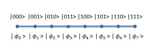
The first register contains qubits in the binary representation of the grid point number and the second register contains qubits with the data associated with that grid point. The data is encoded as in fix or floating point arithmetic. If (3) represents the numerical solution to equation (1) a readout of the index and data registers will reveal a high resolution solution at a randomly selected point in the computational domain. If some particular region is of greater interest quantum amplitude amplification hoyer can be used to to increase the amplitude of states in that region.
In other algorithms (see e.g. linear) the data is encoded in the amplitudes of the quantum states. One problem with that approach is that it is difficult to determine high resolution data samples at specific locations in the computational domain since one would need a very large number of samples to get an accurate probabilistic reconstruction of the state. It is also possible to deploy highly efficient classical multigrid based methods (see lubasch) to problems of type (1).
II multigrid
The most important part of the multigrid algorithm is the V-cycle in which information is propagated between a hierarchical sequence of grids with different resolution. The number of V-cycles required to reduce the residual below a given accuracy , for problems of type (1), is (see demmel). Assume that a starting state has been prepared. The index register can be easily generated by applying Hadamard transformations on each index qubit. The data register could be left in the state or generated using some classical function that takes the index as input.
Next, a multigrid V-cycle (Algorithm 1) is applied in order to improve the starting guess. The V-cycle relies on three operators: the restriction operator that maps from a fine grid (level ) to a coarse grid (level ), the interpolation (prolongation) operator that maps from a coarse grid to a fine grid, and the smoothing (solution) operator that improves the solution and damps high frequency errors. For the lowest level an exact solution to the discretized problem is generated. This condition can be relaxed to requiring a solution with high accuracy, which can be generated, e.g., by applying several iterations of the solution operator. The smoothing operator is often implemented as a Jacobi or Gauss-Seidel type iteration. One possible choice for the different operators in the 1D setting is
| (4) | |||||
| (5) | |||||
| (6) |
Here, it has been assumed that each additional level doubles the number of grid points. Note that for a given point in the computational domain all three operators can be implemented as nearest neighbor actions. In other words, if grid point has access to the data registers and all steps in Algorithm 1 can be performed at this grid point. If a Jacobi type smoother is used these operations can be performed by exploiting quantum parallelism at all grid points in operations.

Since a very high resolution discretization is possible a simple Cartesian grid can be used. For this type of grid it is straightforward to generate the elements of and on-the-fly for many types of computational problems. For the boundary values an oracle is assumed that returns the boundary value based on cell index.
III Quantum data register sharing
From the previous section it is clear that the crucial part of any quantum multigrid algorithm is the sharing of information in the data registers between grid points in the computational domain. In this section a method is outlined for performing this task.
.
Some comments to the above algorithm. For data registers consisting of more than a single qubit, the algorithm can simply be repeated for all qubits in the data register. The Grover diffusion operator can be implemented recursively as . In a similar fashion, can be implemented as , where is a Hadamard gate acting on the index register. The three-qubit phase estimation part of Algorithm 2 requires 7 controlled applications of the Grover diffusion operator. Each Grover diffusion operator requires two applications of , as already observed. Assuming that the other steps of Algorithm 2 requires qubits in total, the resulting complexity of Algorithm 2 is therefore , where is the complexity of and is the accuracy of the data register.
IV Quantum Jacobi
In order to show how the sharing algorithm in the previous section can be used for iterative linear equation system solvers, a simple example is presented in this section. The 1D Poisson’s equation with Dirchlet boundary conditions (1) is solved with the Jacobi method on a regular grid with four grid points. To make the situation more tangible, we may assume that the problem is to calculate the temperature in a rod with fixed cross-section when the temperature at the endpoints is known. In discrete form, using the discretization (2), the left hand side matrix of this problem is
The right hand side vector is , where ans are the boundary conditions (temperatures) at the endpoints. Assume that the starting state of the solution is a vector A solution step of the Jacobi method for this problem consists of updating all element of the solution vector according to
| (7) |
The quantum version of this problem starts with preparing the state
| (8) |
The first register consists of two qubits and encodes the computational grid point on binary form. It is straightforward to prepare this state with a sequence of Hadamard gates. The second register is a k-qubit register that holds the data, in this case the temperature, encoded in fix or floating point arithmetic. At this stage, the data register will hold a starting guess (that can be efficiently prepared) to the problem. This could for example be a constant temperature, or some function that takes the index register as input and returns a temperature at that grid point location. The third register is a working register, containing multiple qubits, possibly in a superposition. We may assume that the preparation of (8) is performed with an operator :
| (9) |
where the index register has been written in decimal form. In order to implement the Jacobi step (7) it is clear that each state (except the endpoints) in the superposition (8) needs information from its two neighboring states. In order to share information between states, Algorithm 2 is used repeatedly. Writing , the operator , where is a Hadamard gate acting on the last bit of the index register, implements the Grover diffusion operators , for terms 0 and 1, and 2 and 3 of , respectively. Let denote steps 1-10 in Algorithm 2.
| (10) |
Calculate the shared values accoring to step 11 in Algorithm 2 and copy the results to a new register with a quantum algorithm
| (11) | |||||
The values and have now been shared between the first two states in the superposition. In the same way and have now been shared between the last two states in the superposition. Next, the values and have to be shared between states 1 and 2 in the superposition. Apply a cyclic (right) shift on the index register, mapping . After regrouping terms:
| (12) | |||||
In order to simplify the notation, the states have been absorbed in the working register, increasing its length to . It can be verified that the Grover diffusion operators for this state can be implemented as for . Share the register values with Algorithm 2 again:
| (13) | |||||
By again utilizing step 11 in Algorithm 2 and copying the results to a new register with a quantum algorithm , applying a cyclic left shift and absorbing garbage in the working register the resulting state is
| (14) | |||||
Now, assuming that the elements of left hand side matrix and the right hand side vector can be efficiently calculated, everything is in place for the Jacobi step J.
| (15) |
This is of the same form as (8) and the process can be repeated.
V Quantum multigrid
It is obvious that the example in the previous section can be extended to registers of arbitrary size. Also, since the multigrid operators (4) - (6) only rely on nearest neighbor action, the same approach can be used to implement these operators. However, in order to implement the full multi grid algorithm in an efficient way, a number of assumptions have to be introduced. Denote the exact solution vector to the problem , with elements . Let be the operator that takes the problem from the starting state to the state after multigrid V-cycle . In order to prevent the complexity of the Grover diffusion operators to increase exponentially, we consider cases for which there exists an efficient approximation , such that,
| (16) | |||||
| (17) |
where the complexity of is at most the complexity of plus a constant. For small numbers and ; the amplitudes are assumed to satisfy
| (18) |
the states are superpositions of norm 1 that satisfy
| (19) |
for some pure states that are close enough to in a fix or floating point arithmetic sense, according to
| (20) |
is now a garbage register that can be an arbitrary superposition of norm 1 that does not have to be close to . From equation (20) it can be deduced that the number of multi grid V-cycles needed to reduce the residual below a given accuracy , for problems of type (1), changes from to . In order to prevent the states in the superposition (16) to decay too much, and have to satisfy
| (21) |
The above assumptions cannot be expected to hold in the general case. Therefore, it is important to identify cases where they might be applicable. Real-world problems usually satisfy some degree of smoothness. For reasonably well behaved problems it can be expected that the solution vector can be compressed with classical (lossy) signal compression algorithms such as Fourier or Wavelet transforms. This assumption is also used in lubasch. More precisely, we will assume here that there exists a function , that can be implemented efficiently with a classical circuit, that takes an index , such that
| (22) |
in time for all elements in the solution vector . A quantum circuit can be constructed by preparing states in an equal superposition according to equation (3) and then applying to each state in parallel. Obviously, is an efficient approximation for the full quantum multi grid algorithm. It is conjectured here that for problems that satisfy this property, also the intermediate solution vectors after each V-cycle can be approximated efficiently according to (17) - (20), with a number of quntum gates that is polynomial in . To summarize, for the class of problems discussed here, there exists a quantum circuit that implements the full quantum multi grid algorithm with an exponential speedup compared to the best classical algorithm (classical multigrid). However, we have so far only discussed the existence of the efficient approximations but not how to construct them. In other words, we know that a certain quantum circuit can be compressed but we do not know how to perform this compression. It has to be assumed that, given their existence, a quantum compiler can construct from in a time that is polynomial in the number of qubits. It is currently not clear how to achieve this.
Acknowledgments
I’m grateful to Anargyros Papageorgiou for very helpful discussions and comments.
References
- (1) Giles Brassard, Peter Hoyer, Michele Mosca, Alain Tapp. Quantum Amplitude Amplification and Estimation. arXiv:quant-ph/0005055
- (2) Aram W. Harrow, Avinatan Hassidim, Seth Lloyd. Quantum algorithm for solving linear systems of equations. Physical Review Letters, volume 15, pp. 150502 (2009)
- (3) Michael Lubasch, Pierre Moinier, Dieter Jaksch. Multigrid renormalization. Journal of Computational Physics, volume 372, pp. 587 (2018)
- (4) James W. Demmel. Applied Numerical Linear Algebra. pp. 331-347 (1997)
- (5) Anupam Prakash. Quantum Algorithms for Linear Algebra and Machine Learning. http://www.eecs.berkeley.edu/Pubs/TechRpts/2014/EECS-2014-211.html