A finite element method to a periodic steady-state problem for an electromagnetic field system using the space-time finite element exterior calculusJournal: Jounal of LaTeX Templates
Abstract
This paper proposes a finite element method for solving the periodic steady-state problem for the scalar-valued and vector-valued Poisson equations, a simple reduction model of the Maxwell equations under the Coulomb gauge. Introducing a new potential variable, we reformulate two systems composed of the scalar-valued and vector-valued Poisson problems to a single Hodge-Laplace problem for the -form in using the standard de Rham complex. Consequently, we can apply the Finite Element Exterior Calculus (FEEC) theory in directly to deduce the well-posedness, stability, and convergence. Numerical examples using the cubical element are reported to validate the theoretical results.
Keywords:
Finite Element Exterior Calculus , Maxwell equation , periodic steady state analysis , Hodge Laplacian , Cubical element2020 MSC
65N12, 65N30, 35J251 Introduction
Let be a bounded Lipschitz domain in . We consider the space-time region with a given , and set the lateral boundary . The target problem in this paper is the following coupling problem composed of the scalar-valued Poisson equation, vector-valued Poisson equation, and divergence-free constraint with the essential boundary conditions (see [1]):
| (1a) | ||||||
| (1b) | ||||||
| (1c) | ||||||
| (1d) | ||||||
| (1e) | ||||||
Therein, a scalar-valued function of and denotes the scalar potential, and a vector-valued function of and denotes the vector potential. Assume that the charge density and current density , respectively, are given scalar-valued and vector-valued functions. Moreover, assume that and are continuous and -periodic with respect to the time variable. That is, and for all . The outer unit normal vector to is denoted by . Here and hereinafter, we use the standard notation of the vector calculus. It should be noticed that the function satisfies
Therefore, we call (1c), (1d) and (1e) the vectoe-valued Poission equation with the divergence-free constraint.
Many components and equipments such as motors, engines, turbines, and plasma-based etching and deposition systems are operated in periodic steady-state conditions [1],[2]. The system (1) is a simple reduction model of the Maxwell equations under the Coulomb gauge in a periodic steady-state. Therein, the gradient of the scalar potential denotes the static electric field, and the time derivative of the vector potential denotes the inductively electric field. The performance and lifetime of the plasma source are estimated by the induced electric field and electrostatic field, respectively. Therefore, it is important and challenging for calculating the periodic steady-state described by ((1)) in the plasma equipment simulation.
Although equations (1a) and (1c) are just linear partial equations, their numerical computations have some difficuluties. Problem (1a) and (1b) is the scalar-valued Poisson equation with the homogeneous Direret boundary condition at each time. In the mixed finite element method, we introduce an intermediate variable. The unkowns and are solved, respectively, in the -th order polynomial space and the th order one as a vector-valued function. The combination of and is known to cause issues such as numerical oscillation (see [3]). On theother hand, Equations (1c)–(1e) often appear in static magnetic fields problem at each time. Equation (1d) is called the Coulomb condition and is solved simultaneously with vector-valued Poisson equation () in a mixed formulation using the Lagrange multiplier method. The condition of (1e) is called the metal boundary condition and is a kind of the essential boundary condition Each component of is related each other due to conservation law .
The theory of the Finite Element Exterior Calculus (FEEC) gives a useful framework to solve these problems. Actually, the scalar-valued and vector-valued Poisson problems are formulated by the Hodge Laplacian problem for the -form and -form, respectively, using the standard de Rham complex in (see [4] for example). Applying the FEEC theory, we can derive a mixed weak formulation and constract stable finite element spaces in a coherent manner; see [5] [6] [7]. That is, the scaler-valued Poisson problem (1a)–(1b) and vector-valued one (1c)–(1e) are solved by the stable finite element method separately. We review this point in Section 2. The purpose of this paper is to propose alternate (and somewhat new) approach. We consider as a subset of and formulate (1a)-(1e) as a boundary value problem for the Hodge-Laplacian problem on the 4-dimensional space-time region with a -dimensional potential as an unknown variable. To be more specific, we introduce a new potential as a direct product and express it as
using the dual basis of the canonical basis corresponding to the time variable and the wedge product . If we interpret and as the -form and -form, the new potential becomes the -form in . Moreover, two systems composed of the scalar-valued and vector-valued Poisson problems imply a single Hodge–Laplace problem for the -form in .This is possible because the problem (1) does not contain the time derivative term. Consequently, we can apply the FEEC theory in directly to deduce the well-posedness, stability and convergence. Of course, it is in general difficult to find a suitable finite element space in . We restrict our consideration to the cubical element that is a poroduct of the interval element. This enable us to extend the results for to those for .
The FEEC theory has contributed to the development of higher-order Whitney elements [5, Chapter 7]. Furthermore, FEEC is considered as a unified theory of finite element methods and one of the theoretical bases for the development of structure-preserving schemes in more complex problems [8]. For example, FEEC gives the structure preserving scheme in the calculation of electromagnetic field on the Vlasov-Maxwell system [9]. Here, another approximation theory of differential form, Discrete Exterior Calculus (DEC) [10] is also used for the calculation of the Vlasov-Maxwell system [11]. As an attempt to include the time axis, we know Salamon’s work of Space Time FEEC [12]. Quenneville–Belair dealt with the time evolution problem of Maxwell equations in the 3-dimensional FEEC [13].
This study reports new applications of the FEEC theory. Our novel feature is to utilize a mesh in the 4-dimensional space-time and solve the Hodge Laplacian problem on the 4-dimensional periodic steady condition using the FEEC framework.
This paper is organized as follows. We review the FEEC theory of in §2. In §3, we derive our proposed Hilbert complex and formulate the main problem as Hodge–Laplacian problem. Then, we discuss the well-posedness. In §4, we state a numerical simulation scheme of the Hodge laplacian problem as saddle point problem. §5 shows the numerical examples for support of our theoretical discussion
Notation
We use the standard Lebesgue for and set . The standard Sobolev spaces are also used:
| (2a) | ||||
| (2b) | ||||
| (2c) | ||||
| (2d) | ||||
| (2e) | ||||
| (2f) | ||||
2 Brief review of the FEEC in
Before studying the main target problem (1), we review the FEEC theory using the steady-state version of (1) :
| (3a) | ||||||
| (3b) | ||||||
| (3c) | ||||||
| (3d) | ||||||
| (3e) | ||||||
All functions in this section are supposed to be time-independent. We use the symbols and in the periodic steady-state problem (1) and steady-state problem (3), since there is no fear of confusion. This section is based on [5, Chapters 4 and 5]. In order to state the reformulation of (3) in terms of the exterior calculus, we first recall a suitable Hilbert complex. It should be noticed that the de Rham complex with no boundary condision is disccussed in [5]. In particular, we work on the de Rham complex associated with with boundary conditions. The base Hilbert spaces are , . The operators are defined as , , and with domains , , and , respectively. The domain complex is described as
| (4a) | |||
| or, equivalently, | |||
| (4b) | |||
The dual complex is given as
| (5a) | |||
| or, equivalently, | |||
| (5b) | |||
where we have set , , and with domains , , and .
All and are closed densely defined linear operators. Moreover, we have and . That is, we have and . These imply that (4) and (5) are Hilbert complexes (see [5, Definition 4.1]). Furthermore, is the adjoint operator of .
The de Rham complex has the following property ([5, p. 38]).
Proposition 1.
is compactly included in for .
Set
| (6) |
An element is called a harmonic -form, if and . The set of all harmonic -form is denoted by . We know that . It can be verified that, if is simply-connected,
| (7a) | ||||
| (7b) | ||||
Moreover, we have ([5, Theorems 4.5 and 4.6])) the following.
Proposition 2 (Hodg decomposition).
We have the orthogonal decomposition and , where .
Proposition 3 (Poincaré inequality).
There exists a positive constant such that for .
At this stage, the Hodge Laplacian is defined as
| (8a) | |||
| with its domain | |||
| (8b) | |||
The Hodge Laplace problem in a strong form is described as follows: Given , find such that
| (9) |
where denotes the orthogonal projection form onto .
On the other hand, the Hodge Laplace problem in a primal weak form is: Given , find such that and
| (10) |
Finally, the Hodge Laplace problem in a mixed weak form is: Given , find , and such that
| (11a) | ||||||
| (11b) | ||||||
| (11c) | ||||||
In view of [5, Theorems 4.7, 4.8 and 4.9], we know
Proposition 4.
Now, we turn to our steady-state problem (3). First, the problem (3a) and (3b) for finding is nothing but the the Hodge Laplace problem for . For convenience, we assume that is simply-connected. Since , (9) implies that
To interpret (3c)–(3e) for finding in the framework of the Hodge Laplacian problem, we introduce the following problem.
problem: Given , find such that
| (13) |
In essentially the same way as the proof of [5, Theorem 4.12], we prove
Proposition 5.
The problem (3c)–(3e) for finding is equivalent to the problem as long as is taken from . That is, if is given as for some , we have
and
The last assertion follows from .
In summary, the steady-state problem (3) is formulated as
| (14a) | |||
| (14b) | |||
We proceed to the finite element approximation of the Hodge Laplace problem in the mixed weak form (11). We are interested in the case and . Let be a finite dimensional subspace of . Then, we have
On the other hand, for the discrete harmonic forms
we do not know whether
holds true or not. However, we know in our setting
| (15) |
The Galerkin approximation for (11) reads as follows: Given , find , and such that
| (16a) | ||||||
| (16b) | ||||||
| (16c) | ||||||
In particular, if , (16) implies : Given , find such that
| (17) |
If , (16) implies : Given , find , such that
| (18a) | ||||||
| (18b) | ||||||
We make the following conditions on :
- (H1) Subcomplex property.
- (H2) Existence of bounded cohain projections.
-
There exists a linear operator such that and , and the restriction of to is the identity on . In other words, we have the following commuting diagram relating the complex to the subcomplex :
is assumed that is satisfied bounded with uniformly in h and the commutativity .
- (H3) Approximation property.
-
(20)
Under these assumption, we prove (see [5, Theorems 5.4 and 5.5]).
Proposition 6.
Although we do not recall here, many concrete examples of satisfying (H1), (H2) and (H3) are known.
3 Space-time 4D formulation
In the previous section, we reviewed the FEEC frame work using the de Rham complex in . Based on these preliminaries, we introduce a Hilbert complex in the space-time region in to handle scalar-valued and vector-valued potentials simultaneously. We then study the proposed Hilbert complex and the Hodge Laplacian and verify that they give a useful framework to solve the periodic steady-state problem (3).
3.1 Hilbert complex on
In our strategy, the main problem (3) is formulated as a boundary value problem of the Hodge Laplacian problem in the space-time region . To this end, we write
and treat as a subset of . We use the dual basis of the canonical basis and often write . We introduce a potential in that is a direct sum of the scalar-valued potential and the vector potential vector-valued potential and express it as
where the denotes the wedge product. Consequently, the potential is understood as a differential -form on . We recall that and are functions of and . Therefore, should be precisely understood as for any . Similarly, should be precisely understood as for any . Below we will employ the abbreviation and to express these relations. Further, the force field in is defined as a direct sum of the electric field and the magnetic field as , which is a differential -form on .
To treat a differential -form in of the form in a coherent way, we introduce a subset of a vector space of all differential -forms on in the following way. For the time being, we take no care about the smoothness and integrability of differential forms. We set
| (22a) | ||||
| (22b) | ||||
| (22c) | ||||
| Herein, we recall that the abbreviation for any is employed. Their inner products are defined as | ||||
| (22d) | ||||
| where (with ) and stands for the volume form on . The norm is defined as | ||||
| (22e) | ||||
In generally speaking, Minkowsky inner product in the space time leads to indefinite norm and the space is not always Hilbert space [14]. However, the inner product we introduced in 4d space time by enetention of 3d defferntial inner product holds positive defined property. Then, we can introduce
| (23) |
Furthermore, we set for
| (24a) | ||||
| (24b) | ||||
where . We now state the definition of linear operators of with its domain and of with its domain :
| (25a) | ||||
| (25b) | ||||
where or . Using these operators, the spaces and for are expressed alternately as
| (26a) | ||||
| (26b) | ||||
These spaces are Hilbert spaces equipped with the following inner products and norms:
| (27a) | ||||
| (27b) | ||||
| (27c) | ||||
| (27d) | ||||
The inner products and norms for and are defined with obvious modifications. Moreover, and are densely defined closed operators. These properties follows directly from the corresponding properties of and . Then, as a direst consequence of (4) and (5), we have a Hilbert complex,
| (28) |
and the dual complex,
| (29) |
In both complexes, base Hilbert spaces are . In particular, we have and as readily obtainable consequences of and . In view of Proposition 7, and are compactly included in and , respectively. Therefore, we obtain the following.
Proposition 7.
is compactly included in for .
3.2 The periodic steady-state problem (1)
At this stage, we introduce the Hodge Laplacian as
| (33a) | |||
| with its domain | |||
| (33b) | |||
The Hodge Laplace problem in a strong form is described as follows: Given , find such that
| (34) |
where denotes the orthogonal projection form onto . We skip a primal weak form and state the Hodge Laplace problem in a mixed weak form: Given , find , and such that
| (35a) | ||||||
| (35b) | ||||||
| (35c) | ||||||
The following proposition is an application of [5, Theorems 4.7, 4.8 and 4.9] as Proposition 4.
Proposition 8.
As the steady-state problem (3) is equivalent to the -problem of (9), the periodic steady-state problem (1) is equivalent to the problem of the Hodge Laplace problem (34). We explain this fact more precisely. Letting and , we set . Assume that . That is, we assume that and are expressed as and for some and . By Proposition 8, there exists a unique satisfying . Setting
| (37a) | ||||
| we have | ||||
| (37b) | ||||
| (37c) | ||||
| (37d) | ||||
By (37a), (37c) and (37d), we find that and it solves
| (38) |
This implies that is a solution of
| (39a) | |||
| (39b) | |||
for any . That is, is a solution of (1).
4 Finite element approximation
In the previous section, we formulate the periodic steady-state problem (1) as the the Hodge Laplace problem (38) for the differential -form in . Then, we can apply the abstract theory recalled in §2 for the Galerkin approximation. The only thing we leave is to construct concretely a finite dimensional subspace of which satisfy (H1), (H2) and (H3) in §2. In this section, we assume that is a -rectangle in and that we are given a mesh subdivision of composed of -rectangle elements. The size parameter is defined as the maximum length of each .
4.1 Approximation by a cubical element
Let and be integers. We introduce the cubical element (see [15])
| (40) |
where denotes a set of all polynomial defined in of degree and
| (41) |
Using this, we set
| (42) |
with . Then, and are defined similarly for . Actually, they correspond to the case .
Theorem 1.
The space can be identified with for any .
Proof.
It is verified by a direct calculation. For example, is expressed as
where and . Therefore, . The converse is the same. ∎
We now introduce a finite element space for as
| (43) |
We have
and the discrete harmonic form is defined as . In our setting,
| (44) |
Then, the finite element approximation of (35) reads as follows: Given , find , and such that
| (45a) | ||||||
| (45b) | ||||||
| (45c) | ||||||
Theorem 2.
- (a)
The space has the approximation property;
- (b)
The space has the subcomplex property; and .
- (c)
There exists a bounded cohain projection ; The following diagram commutes:
Proof.
(a) is a standard fact. (b) follows from a direct calculation. (c) is a consequence of the result for as verified below. Let be a subdivision of by -rectangles such that , we set
According to the explanation in for [5, p.92]. The paper [15] shows the existence of bounded cochain projection following the method of [16]. The case of is also shown to have the bounded cochain projection by exactly same procedure. Therefore, there exists a bounded cochain projection where and the cubical element satisfies the commutativity property: . We set
Then, we have by a direct calculation. ∎
Therefore, we obtain (see [5, Theorems 5.4 and 5.5])
4.2 Reference element
As a concrete example, consider a hypercube with a node element and an edge element as the reference elements in the 4d space-time (see Figure 1). A cube is placed at time . This cube is extruded to along with time direction to make a hypercube. The number of node points is 8+8=16. The cube in the time includes 12 edges, and the cube in the time also consists of 12 edges. Besides, extruded eight nodes make eight edges along with time direction, so the total number of the edge is 32. Hypersurfaces and hypervolumes are also considered in the same way, with 20,1. We consider the differential forms ,0-form and a 1-form , on the reference element . A hyper node reference element have values on the 16 grid points. is considered as following
| (46) | |||
| (47) |

A hyper edge reference element have values on the 32 edges. is considered as following
| (48) |
which,
| (49) | |||
| (50) |
| (51) | |||
| (52) |
| (53) | |||
| (54) |
| (55) | |||
| (56) |
,respectively. The variable of scalar potential is placed on an edge in the time direction and the variable does not contain time.In higher-order elements, time is included at (r-1)-order. The vector potential has a time component, but the differential operator not contribute for time.
4.3 Arrow–Hurwicz Algorithm (AHA)
As is stated in §3.2, the periodic steady-state problem (1) is equivalent to the problem of the Hodge Laplace problem (34);
| (57) |
where . We recall that is defined as . If is given exactly (in a suitable discrete sense), we can obtain the solution by solving the full Hodge Laplace problem (34). However, it is difficult to ensure in the actual computation. Therefore, it is useful to formulate (57) as a saddle point problem of the action defined as
| (58) |
Recall that is called a saddle point of if it satisfies
| (59) |
To be more specific, we state the following theorem.
Theorem 4.
A couple of differential forms is a a saddle point of if and only if it solves the mixed weak form of (57) given as
| (60a) | ||||||
| (60b) | ||||||
Proof.
We have shown that the Hodge Laplacian problem can be formulated as a saddle point problem. After a discretization, the saddle point formulation be written as a matrix form,
| (61) |
Since the coefficient matrix is in general indefinite, a special solver is required. There are many methods for solving matrix equations. In this study, we employed the Arrorw-Hurwicz Algorithm, a kind of Uzawa-type iterative solution method developed in economics [17, 18].
Arrorw-Hurwicz Algorithm (AHA)
- 1.
Chose an initial guess and .
- 2.
For k=0,1,2,…., until convergence of iterative error Do:
- 3.
- 4.
- 5.
EndDo
The matrix is the main part of the Laplacian and contains the scalar Laplacian and the vector Laplacian. The matrix is the term that represents . The potential term has degenerated. Since alone is an indefinite problem, it is an iterative method that oscillates toward the unique saddle point while taking into account.
5 Numerical examples
5.1 Numerical Example 1
We checked the mesh convergence of our proposed scheme under the problem of an exact solution in supper cubic. . The source data is following equation,
| (62) |
The exact solution of this problem is bellow.
| (63) |
This solution satisfied , the vector potentials are toward the boundary face’s normal direction, and is equal to zero on the boundary face. Table 1 shows the dependency of mesh size of error, and the convergence order is .
| (64) |
| 20736 | 0.0833 | 0.15988 | |
|---|---|---|---|
| 65536 | 0.0625 | 0.09132 | 1.94678 |
| 160000 | 0.05 | 0.05886 | 1.968276 |
| 331776 | 0.0041677 | 0.04104 | 1.977904 |
| 614656 | 0.0035714 | 0.03022 | 1.98531 |
The convergence rate is visibly linear under the log-log plot. The numerical example 1 shows optimal second-order convergence.
5.2 Numerical Example 2
We show a practical example for electromagnetic simulation. Figure 2 shows the problem setting of the virtual plasma source.
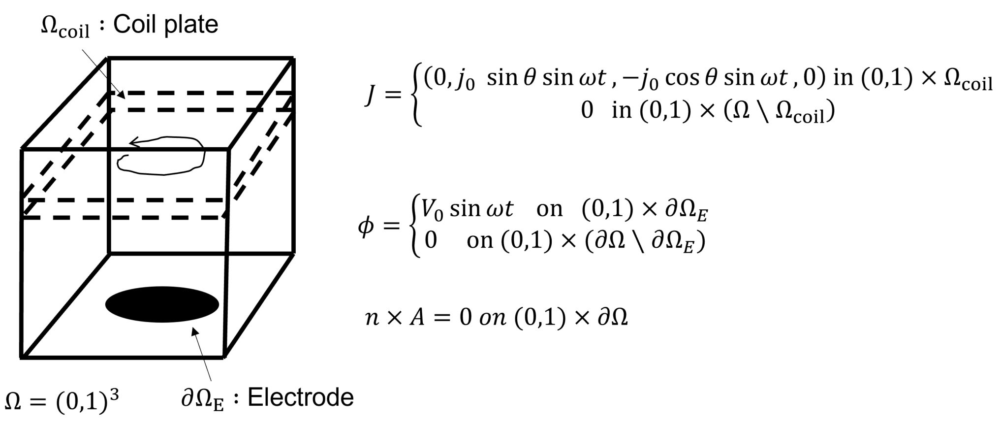
The calculation domain is and . There is no plasma in this case, but it is a shape that could be used as a plasma source for Inductively coupled plasma(ICP) and capacitively coupled plasma(CCP). The electric current() flows around the coil plate, set at the height of z=2/3. The electric charge doesn’t exist. The boundary condition of vector potential is metal boundary condition as . The electrode is set on the bottom and applied the sinusoidal wave(). The other boundary condition of the scalar is grounded(). Our theoretical discussion was performed under the zero boundary condition. However, exaple2 is a more complex boundary condition because we can obtain a reasonable solution under the more practical checking problem setting. Fig.3 and Fig.4 show the calculation results of the scalar and vector potential distribution by the cross-sectional view of x=0 under the coarse and fine mesh.


The 1st order(r=1) elements of space-time are used. However, the visualization is performed as the average value of each element, and the scalar and the vector potential are separated. It can be confirmed that the solution satisfies the discrete maximum principle with the maximum value at the electrode, depending on the change in the sine waveform given to the electrode. As for the vector potential, a tendency was obtained that it is parallel to the current direction, and its absolute value rapidly decreases as it moves away from the coil plate. Figures 5 and 6 show the calculated scalar and vector potentials on the (x=0) cross section under the coarse and fine meshes.


The results show that the vector potential is generated in a vortex. In the boundary condition problem, the intensity of the solution increases from the center to the outside, but since the tangential direction of the boundary is zero and the vector value on the boundary has only a normal component as the metal boundary condition, the absolute value of the intensity decreases toward the normal direction as it moves outward.
6 Conclulding Remarks
In this paper, the periodic steady-state of electromagnetic fields is calculated using differential forms in 4-dimensional space-time. In the conventional method, the scalar potential 0-form and the vector potential 1form are considered separately on the three-dimensional de Rham Complex. In the proposed formulation, the scalar potential 0-form and the vector potential 1-form are treated simultaneously as 1-form in the 4-dimensional spacetime. We consider a direct product space by the shifted differential -form and the differential -form and its Hilbert Complex. And the proposed formulation is equivalent to the weakly mixed formulation of the Hodge-Laplacian in the 4-dimensional spacetime. Then, the wellposedness of this 4-dimensional Hodge-Laplacian is shown using the FEEC framework. For the function space of the discrete solution, we considered the direct product space of shifted (k-1)-form space(cubical element space) in the 3-dimension and k-form space(cubical element space). It was also shown that this product space coincides with the 4-dimensional cubical element space. The unbounded cochain map between a 4-dimensional complex and its approximate complex exists by using the approximate map from the cubical element spaces to the differential form space on the 3-dimensional space. Then, we show the well-posedness of the formulation of the weakly mixed problem using the framework of FEEC theory.
We have tested the proposed method on two example problems. The example 1, the exact solution exists, the discrete solution converges to the exact solution in optimal order by the proposed method. The more concrete example2 shows that the proposed method can solve problems with non-zero boundary conditions for the scalar potential. These results support our theoretical analysis and the usefulness of our proposed method. In this paper, we have focused on a model in which the time derivative term is neglected. In the future, it is expected that calculate Maxwell’s equations with time terms taken into account and develop another periodic steady problem such as fluid fields Furthermore, extend to the coupled problems of electromagnetic and fluid fields for plasma simulation.
Acknowledgement
I’d like to thank for flutiful disscusion with Dr. Masaru Uchiyama.
References
- [1]
J. D. Jackson, Classical
electrodynamics, 3rd Edition, Wiley, New York, NY, 1999.
URL http://cdsweb.cern.ch/record/490457 - [2] M. A. Lieberman, A. J. Lichtenberg, Principles of plasma discharges and materials processing, John Wiley & Sons, 2005.
- [3]
D. Boffi, F. Brezzi, M. Fortin,
Mixed finite element methods
and applications, Vol. 44 of Springer Series in Computational Mathematics,
Springer, Heidelberg, 2013.
doi:10.1007/978-3-642-36519-5.
URL https://doi.org/10.1007/978-3-642-36519-5 - [4]
L. W. Tu, An introduction to
manifolds, 2nd Edition, Universitext, Springer, New York, 2011.
doi:10.1007/978-1-4419-7400-6.
URL https://doi.org/10.1007/978-1-4419-7400-6 - [5]
D. N. Arnold, Finite element
exterior calculus, Vol. 93 of CBMS-NSF Regional Conference Series in Applied
Mathematics, Society for Industrial and Applied Mathematics (SIAM),
Philadelphia, PA, 2018.
doi:10.1137/1.9781611975543.ch1.
URL https://doi.org/10.1137/1.9781611975543.ch1 - [6]
D. N. Arnold, R. S. Falk, R. Winther,
Finite element exterior
calculus, homological techniques, and applications, Acta Numer. 15 (2006)
1–155.
doi:10.1017/S0962492906210018.
URL https://doi.org/10.1017/S0962492906210018 - [7]
D. N. Arnold, R. S. Falk, R. Winther,
Finite element exterior
calculus: from Hodge theory to numerical stability, Bull. Amer. Math. Soc.
(N.S.) 47 (2) (2010) 281–354.
doi:10.1090/S0273-0979-10-01278-4.
URL https://doi.org/10.1090/S0273-0979-10-01278-4 - [8]
S. H. Christiansen, H. Z. Munthe-Kaas, B. Owren,
Topics in
structure-preserving discretization, Acta Numer. 20 (2011) 1–119.
doi:10.1017/S096249291100002X.
URL https://doi.org/10.1017/S096249291100002X - [9] M. Kraus, K. Kormann, P. J. Morrison, E. Sonnendrücker, Gempic: geometric electromagnetic particle-in-cell methods, Journal of Plasma Physics 83 (4).
- [10] A. N. Hirani, Discrete exterior calculus, Ph.D. thesis, California Institute of Technology, 2003.
- [11] J. Squire, H. Qin, W. M. Tang, Geometric integration of the vlasov-maxwell system with a variational particle-in-cell scheme, Physics of Plasmas 19 (8) (2012) 084501.
- [12] J. Salamon, J. Moody, M. Leok, Space-time finite-element exterior calculus and variational discretizations of gauge field theories, in: 21st International symposium on mathematical theory of networks and systems. Groningen, The Netherlands, Citeseer, 2014.
- [13] V. Quenneville-Belair, A new approach to finite element simulations of general relativity, Ph.D. thesis, University of Minnesota, 2015.
- [14]
P. Petersen, Riemannian
geometry, 3rd Edition, Vol. 171 of Graduate Texts in Mathematics, Springer,
Cham, 2016.
doi:10.1007/978-3-319-26654-1.
URL https://doi.org/10.1007/978-3-319-26654-1 - [15]
D. N. Arnold, D. Boffi, F. Bonizzoni,
Finite element differential
forms on curvilinear cubic meshes and their approximation properties, Numer.
Math. 129 (1) (2015) 1–20.
doi:10.1007/s00211-014-0631-3.
URL https://doi.org/10.1007/s00211-014-0631-3 - [16]
S. H. Christiansen, R. Winther,
Smoothed projections in
finite element exterior calculus, Math. Comp. 77 (262) (2008) 813–829.
doi:10.1090/S0025-5718-07-02081-9.
URL https://doi.org/10.1090/S0025-5718-07-02081-9 - [17]
Y. Saad, Iterative methods for
sparse linear systems, 2nd Edition, Society for Industrial and Applied
Mathematics, Philadelphia, PA, 2003.
doi:10.1137/1.9780898718003.
URL https://doi.org/10.1137/1.9780898718003 - [18] K. J. Arrow, H. Azawa, L. Hurwicz, H. Uzawa, Studies in linear and non-linear programming, Vol. 2, Stanford University Press, 1958.