Constraint Learning to Define Trust Regions in Predictive-Model Embedded Optimization
Abstract
There is a recent proliferation of research on the integration of machine learning and optimization. One expansive area within this research stream is predictive-model embedded optimization, which proposes the use of pre-trained predictive models as surrogates for uncertain or highly complex objective functions. In this setting, features of the predictive models become decision variables in the optimization problem. Despite a recent surge in publications in this area, only a few papers note the importance of incorporating trust region considerations in this decision-making pipeline, i.e., enforcing solutions to be similar to the data used to train the predictive models. Without such constraints, the evaluation of the predictive model at solutions obtained from optimization cannot be trusted and the practicality of the solutions may be unreasonable. In this paper, we provide an overview of the approaches appearing in the literature to construct a trust region, and propose three alternative approaches. Our numerical evaluation highlights that trust-region constraints learned through isolation forests, one of the newly proposed approaches, outperform all previously suggested approaches, both in terms of solution quality and computational time.
Keywords: Data-driven decision making; integration of machine learning and optimization; trust region; constraint learning; isolation forest
1 Introduction
The use of pre-trained predictive models in optimization decision problems is nothing new. In this setting, the collected data includes a set of controllable independent variables as past decisions (sometimes together with uncontrollable variables) and their corresponding outcomes. Practitioners benefit by learning from data to make decisions that result in more favorable outcomes [Biggs et al. 2017, Mišić 2020] through surrogate models, to learn the underlying relationship between the controllable independent variables and their outcome [Biggs et al. 2017, Grimstad and Andersson 2019a]. Once the relationship is learned, one can solve an optimization problem defined over the predictive model, where decision variables in the optimization problem correspond to the controllable independent variables, and the objective function is given by the outcome of the pre-trained predictive model. We will refer to this decision-making paradigm as predictive-model embedded optimization (PMO).
Examples abound; consider a traditional setting in advertising. Suppose a retailer can select from among advertising channels. Given a budget of dollars, how much should the retailer allocate to each advertising channel to maximize revenue? Classical Operations Research methods suggest that a predictive model such as regression model can be fit on historical data (including both previous decisions, market conditions, and revenue) to predict revenue, and then the allocation decision variables can be selected to maximize predicted revenue. Depending on the predictive model chosen, the optimization model can be appropriately formulated. For example, if the predictive model chosen is a linear regression, the optimization problem can be modeled as a linear programming model; if the predictive model chosen is a neural network or a random forest, recent research shows how a mixed-integer model can be formulated (for instance, Anderson et al. 2020).
Because of its generality, PMO finds potential applications throughout the analytical landscape. There is a major issue with the real-world application of PMO, which practitioners are well aware of: decisions produced by PMO are often unrealistic because they can be very different from what is observed historically in data. This happens because often the existing PMO frameworks ignore the trust region, i.e., ensuring that solutions to the optimization problem are similar to the data used to train the predictive models [Maragno et al. 2021, Mistry et al. 2021, Schweidtmann et al. 2022].
Let us demonstrate this issue using an example in a wine production context on a dataset that has been used before in the PMO literature [Mišić 2020, Wang et al. 2021]. Wine scores are typically used by critics to specify their opinion about wine quality. Suppose a wine producer is equipped with a dataset that includes physicochemical property measurements of varieties of wine as features (e.g., pH, fixed acidity, residual sugar, etc.) along with the corresponding wine scores. The producer wants to leverage this dataset and build a PMO model to determine the best combination of physicochemical property measurements that maximizes the expected wine score.
Figure 1 shows a scatter plot (pH versus fixed acidity) for two solutions obtained via a PMO model defined over a trained neural network (which is one of the most popular predictive models nowadays) and historical observations in the data (features are scaled between 0 and 1). The first solution is obtained by solving the corresponding optimization model without additional constraints (represented by an orange cross) and the second solution is obtained by incorporating trust-region constraints (represented by a blue diamond). Measurements of pH and fixed acidity in historical observations present a negative correlation, which is expected as higher acidity should correspond with a lower pH. The initial solution obtained, however, completely violates this relationship, rendering the solution unacceptable. Alternatively, the second solution is closer to the training data and aligns with the aforementioned chemical considerations. It may be argued that the predictive model is not good enough to capture the inverse correlation. However, in predictive modeling applications, a predictive model is usually selected based on its overall predictive performance instead of considering such specific correlation relationships between pairs of features. By solving an optimization problem defined over such a predictive model, we cannot guarantee that the solution obey the practical requirements. In fact, it is a common character of solutions of PMOs falling at the extremes of the feasible region [Maragno et al. 2021].

The example above highlights how the solutions obtained by PMO can be inappropriate for a particular application. That is not the only potential issue. Even if a wine could be created that has the relationship of high acidity and high pH, the evaluation of the objective function of the pre-trained model at that point would be untrustworthy. If the optimization problem selects a solution that is too different from the training data of the predictive model, one cannot trust the prediction produced by the predictive model at that point (i.e., the error is immeasurable). This is well known in the application of predictive modeling, where it is common to assume that the unobserved/test data comes from the same distribution as the historical/training data.
There are therefore two major issues with a direct application of PMO as presented thus far in this paper: (1) the solutions can be inappropriate for the application, and (2) the validity of the predictive model at the solution obtained could be untrustworthy. To address these issues, constraints can be added for each possible application to ensure that the decisions model physical or other real-world considerations, but these relationships might be highly non-linear, or perhaps unknown to the modeler. One might also try to examine all pairs of variables and make sure they are reasonably correlated as desired, but this can be challenging to identify for higher degree relationships and can lead to over constraining.
Recently, some research has focused on developing methods to incorporate trust region in PMOs. For instance, Biggs et al. 2017 and Maragno et al. 2021 use the convex-hull of observations in the dataset to model a trust region, while Schweidtmann et al. 2022 utilize a one-class support vector machine (SVM) to determine constraints for the trust region. In essence, constructing a trust region for PMOs ensures that the solutions are not outliers compared to the historical observations. In this paper, we provide an overview of the existing methods for modeling the trust region in PMOs and explore three additional ways to detect outliers, which are melded into PMOs as a trust region: the first defines a trust region by selecting queries from a pre-trained isolation forest [Liu et al. 2008]; the second uses Mahalanobis distance [Mahalanobis 1936] to constrain the solutions within a given distance of the training data, which is particularly useful when an assumption on multivariate normality is reasonable; and the third incorporates constraints to ensure that the solution is within a limited distance of K-nearest neighbors [Altman 1992] in the training data.
We design computational experiments to compare the performance of our proposed trust-region constraints to the existing approaches in the literature. To our knowledge we are the first to evaluate different trust regions against each other both in terms of solution quality and computational performance (measured in solution resolution time). For our experiments, we generate a testbed of problem instances based on 7 different benchmark functions and use multiple predictive models to fit the training data within our PMO approach. Our results indicate that our proposed constraints compare favorably with the existing approaches from the literature, particularly our Isolation-Forest constraints.
Our contributions are therefore as follows:
- 1.
Although researchers have independently developed methods for modeling the trust region in PMOs, to our best knowledge, we are the first to provide a comparison of existing methods in terms of solution quality and CPU time.
- 2.
We propose three alternative methods for modeling the trust region in PMOs. Our results show the effectiveness of our proposed approaches, particularly the trust region defined by Isolation Forest, compared to existing ones in the literature both in terms of solution quality and computational times.
- 3.
We present a set of benchmark instances that can be used by the optimization community for further research on related topics.
2 Literature Review
Multiple works from the literature consider optimization problems defined over trained predictive models, ranging from simple linear regressions to more complex predictive models such as random forest and neural networks. Bertsimas et al. 2016 optimize over an estimated ridge regression model seeking to improve the efficacy of chemotherapy regimens in clinical trials. Huang et al. 2019 and Baardman et al. 2019 propose optimization models defined over linear regressions in the context of retailers location decisions and scheduling of promotion vehicles, respectively. Ferreira et al. 2016 use random forest to estimate the demand of a product based on its price, and develop an optimization model over a trained random forest to determine product prices that maximize total expected revenue. Other application areas include food delivery Liu et al. 2020, scholarship allocation Bergman et al. 2022, personalized pricing Biggs et al. 2021, and auctions Verwer et al. 2017.
Optimization problems defined over trained predictive models are often challenging to solve, depending on the properties of the underlying predictive model. Mišić 2020 and Biggs et al. 2017 propose exact solution approaches for optimization problems defined over tree ensembles. Mixed integer programming (MIP) formulations for optimization models defined over trained neural networks are studied by Cheng et al. 2017, Fischetti and Jo 2018, Bunel et al. 2018, Dutta et al. 2018, Bergman et al. 2022, Grimstad and Andersson 2019a, Schweidtmann and Mitsos 2019, Tjeng et al. 2019, Grimstad and Andersson 2019b, Botoeva et al. 2020, Anderson et al. 2020 and Tsay et al. 2021. Ensembles of neural networks are studied by Wang et al. 2021. A closely related research area deals with so-called verification problems, which seek to verify relationships between the inputs and outputs of neural networks, as well as to measure the sensitivity of the outputs to small changes in the inputs. These problems are often formulated as mixed-integer programs defined over trained neural networks [Lomuscio and Maganti 2017, Cheng et al. 2017, Katz et al. 2017, Serra et al. 2018].
In predictive modeling, it is common to assume that the unobserved/test data comes from the same distribution as the historical/training data, which is used to build predictive models [Amodei et al. 2016], otherwise the predictive models’ applicability would be limited. Similarly, a solution obtained via PMO can be seen as a new observation in the dataset. The prediction provided by the predictive model should only be trusted if the solution comes from the same distribution as the training data. To constrain the predictive models from extrapolating, a few recent studies have considered the notion of trust region in PMOs. Teixeira et al. 2006 use a clustering technique to define a trust region of a nonparametric input space where the predictions of the predictive model are reliable. Biggs et al. 2017 and Maragno et al. 2021 define a similar subspace using the convex hull of observations in the training data to model a trust region by constraining PMO solutions to be within this convex hull. Mistry et al. 2021 add a penalty term to the objective function so that solutions that lie far away from the subspace constructed by principle component analysis (PCA), are penalized. Schweidtmann et al. 2022 constrain the solutions to belong to a validity domain defined by a pre-trained one-class SVM, a classifier for outlier detection.
3 PMO with Trust-Region Constraints
We consider a trained predictive model that is established to learn the relationship between a dependent variable and a vector of independent variables based upon a set of historical observations . We refer to set as the training input data of the problem and refer to the components of vector as features with index set given by . For simplicity, we assume that all the independent variables are continuous and each independent variable is scaled to . We define decision variables to determine the value of each independent variable and let the predicted outcome of the predictive model be given by . We study problems of the following form:
| (1a) | ||||
| s.t. | (1b) | |||
We consider three different predictive models associated with function : linear regression (LR), random forest (RF), and neural networks (NN). The mathematical formulations corresponding to each one of the three predictive models are discussed in Appendix A. Constraints are then added to the model above to ensure that solutions found are within a trust region. In Section 3.1 we first review three existing types of trust region constraints from the literature. We then introduce our proposed constraints in Section 3.2.
3.1 Overview of the Existing Trust-Region Constraints
3.1.1 Convex Hull Constraints
Maragno et al. 2021 characterize a trust region using the convex hull (CH) of the training input data , which is the smallest convex polytope that contains all the points in . For each sample point in , an auxiliary decision variable is added to describe the convex hull. Let be the index set of . The trust region is then represented by the following constraints:
| (2a) | |||||
| (2b) | |||||
| (2c) | |||||
which ensure that any PMO solution belongs to the convex hull of the training input data.
3.1.2 One-Class SVM Constraints
One-class SVM is an unsupervised machine learning algorithm that specifies a boundary to classify sample points for outlier detection. In other words, if a sample point falls outside of the boundary learned through one-class SVM, it is classified as an outlier. The boundary is mathematically represented using a decision function which may take various forms. The form of the decision function depends on the type of kernel function used to model the data. In SVMs, a kernel is a function that is used to transform the data into higher dimensions so that data points can be linearly separable [Hofmann et al. 2008]. Depending on the complexity of the data, different kernel functions such as linear, polynomial, and Gaussian, among others may be used. It has been shown that complex boundaries can be accurately modeled using a Gaussian radial basis kernel [Tax 2001]. Let denote the set of support vectors from the training input data. A decision function based on a Gaussian radial basis kernel is:
| (3) |
where hyper-parameter is tuned before the training process, while parameters and are learned during the training process for one-class SVMs [Schölkopf et al. 1999].
Schweidtmann et al. 2022 propose trust-region constraints based on one-class SVM classifiers as the ones described above. These constraints ensure that PMO solutions fall inside a trust region and are modeled as:
| (4) |
which ensure that solutions are not classified as outliers by the pre-trained one-class SVM classifier.
PMO models with trust region SVM constraints (4) can be solved directly with off-the-shelf mixed-integer non-linear programming solvers such as BARON [Sahinidis 2017]. To boost the running time performance of this model, we alternatively propose a heuristic branch-and-cut algorithm that enforces trust-region SVM constraints (4) dynamically by checking if PMO solutions violate these constraints via callbacks. Our experiments show that even if the branch-and-cut algorithm is not able to prove optimality, it is able to find high quality solutions quickly. We present the details of this heuristic algorithm in Appendix appendix B.
3.1.3 Principal Component Analysis Constraints
Mistry et al. 2021 incorporate the trust region into PMOs by penalizing solutions that are far away from the training input data. To fulfill this idea, they first define a subspace of the training input data that is created using principal component analysis [Jolliffe 2002] and then include a convex penalty term to penalize the objective function based on the solution’s distance to the defined subspace.
Specifically, given a training input data with features, PCA defines a set of ordered and orthogonal principal components, . Among all the principal components, oftentimes the top (such that ) principal components, , are able to explain most of the variance in . The resulting subspace of is a vector denoted by . Mistry et al. 2021 use the following penalty term to penalize the solutions that are far away from the desired subspace:
| (5) |
where is a non-negative penalty parameter, is the identity matrix, is the sample mean and is the sample standard deviation. Note that PCA is calculated with standardized since it is sensitive to scaling, and is standardized using so that and PCA are in the same scale.
In order to compare Mistry et al. 2021 penalty method of enforcing a trust region with the other constraint-based approaches surveyed, we model the trust region given by PCA with the following constraint:
| (6) |
where threshold is a parameter that controls the looseness (tightness) of the constraint.
3.2 Our Proposed Trust-Region Constraints
We propose three types of trust-region constraints based on three additional techniques used to identify outliers.
3.2.1 Isolation Forest Constraints
Our first proposed type of trust region constraints are originated from a pre-trained isolation forest classifier [Liu et al. 2008], which is a model used for outlier (anomaly) detection.
An isolation forest is an ensemble of isolation trees where each isolation tree is trained over a randomly selected subsample of the training data. An isolation tree is a model that detects outliers using independent variables by checking a series of splits. A split specifies a condition on a single feature using a query of the form “Is ?”, where is a random value within the domain of feature . The series of splits arrange a tree, with each split node branching into two child nodes. To determine whether a data point is an outlier, we start from the root node of the tree and recursively check the query of each split node. If the condition is true, the data point is assigned to the left branch of the split node, otherwise it is assigned to the right branch of the split node. The data point eventually is assigned to a leaf node, for which there are no more splits.
An isolation tree uses a predetermined threshold, , associated with the depth of the leaf nodes. Data points that are assigned to leaf nodes with depth smaller than or equal to are classified as outliers. Figure 2 illustrates an example of an isolation forest classifier having . Leaf nodes with depth smaller than or equal to 2 correspond to data points that are classified as outliers, while leaf nodes with depth larger than 2 correspond to data points that are classified as inliers.
| …… | |||
|
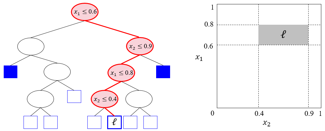
We propose trust-region constraints to ensure that solutions are not classified as outliers by a pre-trained isolation forest. The goal of these constraints obtained from an isolation forest is to ensure that PMO solutions do not correspond to any leaf node with a shallow depth, i.e., a depth less than or equal to . We remark that any solution vector corresponds to exactly one leaf node in each isolation tree and because there is a unique path between the root node of a tree and each leaf node, then leaf nodes correspond to a series of lower and upper bounds on the variable features, given by the queries associated with split nodes in the path from the root node. Figure 3 illustrates the relationship between paths in an isolation forest and variable features bounds. We exploit these bounds to formulate our trust-region constraints as follows.
Consider an isolation forest with isolation trees. Let be the set of leaf nodes in tree . We introduce binary decision variable that takes a value of if leaf node from tree is selected. We introduce auxiliary decision variables and to specify the range of each variable feature . We denote the depth of leaf nodes by , and let the lower and upper bounds corresponding to a leaf node be and for all , , and . Our proposed isolation-forest constraints are:
| (7a) | |||||
| (7b) | |||||
| (7c) | |||||
| (7d) | |||||
| (7e) | |||||
| (7f) | |||||
| (7g) | |||||
Constraints (7a) ensure that exactly one of the leaf nodes from each tree in the isolation forest is selected. Constraints (7b) require that the depth of the selected leaf node in each tree is larger than the threshold . Constraints (7c) and constraints (7d) ensure that, for any leaf node that is selected, the domain of the solution is limited to the feature ranges determined by the path leading to that leaf node. Constraints (7e) ensure that belongs to the domain defined by the corresponding leaf nodes selected. The combination of these constraints ensure that solution does not correspond to a leaf node of any tree that can be labeled as an outlier.
3.2.2 Mahalanobis Distance Constraints
In Section 3.1.3, we introduced a distance-based approach to penalizing solutions further away from the training data subspace defined by PCA. Instead of capturing the distance from a data point to a subspace, we propose to use the Mahalanobis Distance (MD) [Mahalanobis 1936], which measures the number of standard deviations between a given point and the centroid of a distribution. MD has been used for detecting multivariate outliers in different application areas such as psychology [Leys et al. 2018], archaeology [Papageorgiou 2020], and geotechnics [Zheng et al. 2021].
We propose a MD constraint that restricts the MD between the solution and the training input data to be less than or equal to a parameter . Let be the MD measure mentioned above, which is calculated as:
| (8) |
where and C denote the mean vector and the covariance matrix of the training inputs, respectively. We propose adding constraint
| (9) |
as a way of modeling the trust region. We remark that for implementation purposes, the squared form of function can be directly inserted into the model and solved via off-the-shelf optimization solvers such as Gurobi [Gurobi Optimization LLC 2020].
Parameter controls the level of conservativeness of the model. Low values for result in a smaller feasible region in which the solution to the optimization problem must be close to the training input data. Larger values for allow the outcome for the optimization model to be farther away from the training distribution. If the training input data follows a multivariate normal distribution, then follows a chi-square distribution with degrees of freedom, where equals the number of dimensions of the training inputs [Johnson et al. 2014]. In practice, a point is commonly labeled as a multivariate outlier if exceeds a chi-square critical value with degrees of freedom at significance level in . As a result, if the training input data follows a multivariate normal distribution, then a natural value for is given by . We remark that in settings in which the training inputs do not follow a multivariate distribution, constraints based on MD can still be useful after tuning the value of .
3.2.3 K-Nearest Neighbors Constraints
Our third class of constraints considers the distance between the solution of the optimization model and the closest points from the input data, denoted as its -nearest neighbors. This is a straightforward way to ensure that the solution is less likely to be labeled as an outlier as the solution will be close to the input data. This type of measures have been widely used for classification and regression problems [Friedman 2017]. Among the multiple measures of distance available, we propose a formulation that considers the -norm distance metric, which computes the sum of the absolute difference of the individual components of the vectors.
Consider a training data set composed of observations for (where is the index set of the observations). We propose a mixed-integer linear formulation that incorporates a constraint that limits the average distance between the solution of the optimization model and its -nearest neighbors to be less than or equal to a parameter . For all and , let auxiliary decision variables and capture the deviation between the component of solution vector and the component of sample point . Let auxiliary decision variables represent the distance distance between and sample point . We introduce auxiliary binary decision variables that take a value of if sample point is one of the nearest neighbors of solution vector , and auxiliary variables to capture the distance between and the nearest point in (for example, captures the distance between and the closest sample point, captures the distance between and the second closest sample point, and so forth). Our proposed formulation of KNN constraints is given by:
| (10a) | |||||
| (10b) | |||||
| (10c) | |||||
| (10d) | |||||
| (10e) | |||||
| (10f) | |||||
| (10g) | |||||
| (10h) | |||||
| (10i) | |||||
where is a sufficiently large constant. Constraints (10a)–(10b) define the -variables, while constraints (10c) -(10d) define the -variables. Note that for , exactly one variable equals 1 and so exactly one constraint (10c) is activated, ensuring that at optimality equals the distance between and the closest sample point. For , then exactly two variables take a value of 1, activating two constraints (10c). As a result, must be greater than or equal to two of the distances between and the sample points, captured by the -variables. At optimality, will be exactly equal to the distance between and the second closest point in the sample. The model follows the same logic for the remaining values of . Finally, constraint (10e) ensures that the average distance to the -nearest neighbors is less than or equal to threshold .
It can be seen that the size of the PMO model with KNN constraints, both in number of decision variables and constraints, grows with the size of the training data (similar to constraints using convex hull of the dataset). Hence, for large data sets solving these models would be challenging for commercial mixed-integer programming solvers. As a heuristic approach, one may only consider the top of the training data when incorporating KNN constraints.
4 Experiments
In order to test the effectiveness of the various approaches, we evaluate the solution quality obtained by solving PMO on a variety of functions with different trust region definitions. Specifically, we utilize standard global optimization functions for which the optimal solution is known to create synthetic datasets. For each function, we randomly sample inputs from multivariate normal distributions to create a training set. For each input in the training set, we evaluate the known function (with noise), and use that to train models to predict the outcome. We can then solve a PMO with the various trust-region constraints.
This allows for a controlled experimental evaluation of the efficacy of each trust region approach. Because we know the optimal value and we can generate a data set for training predictive models, the gap between the solution value obtained via PMO and the optimal value can be calculated easily and compared across the various approaches. Furthermore, we can also compare the best point in the training data with the values obtained through PMO to see if our proposed approaches improve upon the simple best-in-sample solution. Finally, we can also provide an analysis of the solution time to see which trust-region constraints provide the smallest computational burden.
We present two sets of experimental results on two synthetic datasets based on seven global optimization benchmark functions. Given a synthetic dataset generated from a global optimization benchmark function , we first estimate the relationship (which we denote by as in the definition of PMO) between the independent variables (i.e., the decision variables in the optimization problem) and the dependent variable using predictive modeling, then solve the PMO model, record its solution as , and calculate the true objective value at the solution . We evaluate the quality of a solution by calculating the true outcome of the solution (i.e., ), and the optimality error at the optimal solution (calculated as ). Note that we do not report percent optimality gaps because some of the functions have zero and/or negative evaluations at solutions.
All predictive models are trained in Python using the scikit-learn package [Pedregosa et al. 2011], and all optimization models are solved with Gurobi 9.0 [Gurobi Optimization LLC 2020] in Windows 10 on an Intel(R) Xeon(R) Gold 6130 CPU @ 2.10GHz processor with 32 GB RAM.
4.1 Data Generation
We consider seven benchmark functions:
- 1.
Beale: . The global minimum is located at .
- 2.
Peaks: . The global minimum is located at .
- 3.
Griewank: . The global minimum is located at .
- 4.
Powell: . The global minimum is located at .
- 5.
Quintic: . The global minimum is located at .
- 6.
Qing: . The global minimum is located at .
- 7.
Rastrigin: . The global minimum is located at .
Beale, Griewank, Powell, Rastrigin, Qing, and Quintic [Gavana 2022] are commonly used for evaluating global optimization algorithms, and Peaks is a test function in Matlab [The MathWorks Inc 2010].
For each function, we generate points to be used as training data for estimating the relationship by sampling points from a multivariate normal distribution, with mean located at the global minimum point (i.e., for Beale, for Peaks, for Griewank, for Powell, for Quintic, for Qing, and for Rastrigin) and a covariance matrix randomly generated using function make_spd_matrix in scikit-learn. The outcome of each sampled point is the evaluation of the benchmark function, plus randomly generated noise (i.e., ). For each point, the noise is drawn from a zero-mean normal random variable with variance given by a constant , where is the variance of the evaluations of the benchmark function on the sampled points.
For each function, we generate different datasets of points, each generated with a different randomly drawn covariance matrix. Therefore, for 7 global functions, we have 10 collections of input data, for a total of datasets. This creates the first set of data.
For the second dataset, we follow the same procedure, but remove points surrounding the global optimal solution, to evaluate how well the PMO approaches can perform when the optimal value is far away from the training set. In particular, we generate different datasets of points, each generated with a different randomly drawn covariance matrix, but now removing the data within a central region. This is described and evaluated in Section 4.4.
4.2 Predictive Modeling and Optimization Setup
For each dataset, we scale the independent variables to , standardize the dependent variable, and randomly split the dataset into a training set and a test set in the ratio of . Each training set is used to fit three different predictive models: linear regression, random forest, and neural networks, to be used in PMO.
For the configurations of the neurons in neural networks models, we consider a structure with two hidden layers. The number of neurons in each hidden layer ranges in . For each dataset, we select the best neural networks model out of 500 candidates using the GridSearchCV function in scikit-learn. For random forest models, we create a hyper-parameters grid with the number of trees varying in and the maximum depth of the tree ranging in . We try combinations of parameters and select the best model using GridSearchCV . For linear regression models, we simply fit one single model using scikit-learn for each dataset.
The average out-of-sample performance, measured as , of the various predictive models are presented in Table 1. As we can see, the performance of linear regression is typically very poor for these functions due to the degree of nonlinearity, whereas random forest models and neural networks models have much better performance.
[]
| Predictive Model | Beale | Peaks | Griewank | Powell | Quintic | Qing | Rastrigin |
| Linear Regression | 0.029 | 0.023 | -0.009 | -0.022 | 0.053 | 0.055 | -0.017 |
| Random Forest | 0.305 | 0.445 | 0.416 | 0.360 | 0.390 | 0.390 | 0.152 |
| Neural Networks | -0.298‡ | 0.435 | 0.396 | 0.393 | 0.376 | 0.374 | 0.071 |
- ‡
If a single outlier is removed, the is elevated to 0.297.
4.3 Optimization Results
Each predictive model fitted to each synthetic dataset is an instance. For each instance, we compare PMO with the following configurations:
- •
BASE: no constraints
- •
IF: IF constraints
- •
SVM: SVM constraints solved directly using BARON
- •
: SVM constraints solved with our heuristic branch-and-cut algorithm
- •
CH: CH constraints
- •
PCA: PCA constraints. We also run experiments with PCA as a penalty term, the same way as Mistry et al. 2021 propose. We omit these results as they are very similar to the ones reported modeling PCA via constraints.
- •
MD: MD constraints
- •
KNN: KNN constraints
For all the model formulations, as the input data is scaled between 0 and 1, the domain of the decision variables is . For IF, the isolation forest is pre-trained in Python using the scikit-learn package with all the hyperparameters setting as default. We set the tree depth threshold at for datasets based on Beale and Peaks, and for datasets based on Griewank, Powell, Quintic, Qing, and Rastrigin. We pick this parameter by approximately halving the average depth of training points across the trees. For SVM, we train the one-class SVM classifier using the scikit-learn package in Python. The hyperparameter is set as default in the training step. For , we set the number of pieces of the discretized ranges . For PCA, since the training datasets are not in high dimensions, we set the number of leading vectors ( is the number of independent variables in the training datasets) to make sure that a subspace is defined and meanwhile it can explain the majority of the variance in the training data, and set . For MD we set significance level at , i.e., , as the input data follows a multivariate normal distribution. For KNN, we set and . In a tuning process, we set to only use the top 10% of the data (based on their value of their dependent variable) for formulating KNN constraints.
4.3.1 Solution Outcome Quality
We measure solution quality using two metrics: true outcome and optimality error , where denotes the optimal solution obtained via PMO. Table 2 reports the average improvement of solution quality for different PMO variants as compared to the BASE model over the 210 instances tested. Overall, IF is the best performer both in terms of true outcome and optimality error, followed by SVM.
[]
| IF | 73.0% | 81.6% |
| SVM | 62.1% | 75.2% |
| 64.3% | 75.1% | |
| CH | 43.9% | 49.9% |
| PCA | 21.3% | 23.3% |
| MD | 46.2% | 52.4% |
| KNN | 58.2% | 62.5% |
Table 3 reports the average true outcome and the average optimality error for the solutions obtained from the optimization models over all instances, grouped by benchmark function and predictive model. We also report the average true value for the point in the training data with the smallest observed outcome in the training datasets, referred to as ‘Best Sample’. The best-performing model in each combination of benchmark function and predictive model are indicated in bold and underlined for true outcome and optimality error, respectively.
Beale Peaks Griewank Powell Quintic Qing Rastrigin Linear Regression BASE 3408 4980 0.00 2.98 1.04 0.68 30014 31967 3941 7804 1781 2931 260 210 IF 8 293 -2.01 0.45 0.61 0.02 197 278 47 224 94 135 107 6 SVM 3 257 -1.64 0.02 0.76 0.17 605 621 99 1226 80 323 115 22 3 184 -1.80 0.27 0.76 0.15 434 358 83 1029 75 129 106 3 CH 635 1940 -0.07 2.30 1.01 0.42 4994 5002 2565 4411 1037 1376 119 17 PCA 1683 3055 0.00 2.22 1.01 0.51 17540 18234 5234 7744 1699 2563 254 196 MD 35 967 -0.17 1.93 0.89 0.29 4579 4633 2686 4761 1135 1606 130 34 KNN 36 978 -0.69 1.25 0.54 0.07 680 653 584 1991 233 493 101 1 Random Forest BASE 101 598 -6.03 0.76 0.44 0.23 689 1105 196 475 236 329 84 34 IF 2 52 -6.16 0.91 0.09 0.17 30 56 63 34 51 5 58 10 SVM 11 155 -6.03 0.76 0.19 0.06 206 366 76 108 179† 138 77† 7 24 168 -6.02 0.75 0.15 0.11 180 197 69 219 152 145 64 8 CH 101 598 -6.03 0.76 0.38 0.15 490 824 138 411 135 204 68 13 PCA 63 191 -6.35 1.09 0.39 0.18 591 913 232 505 233 317 74 23 MD 26 350 -6.03 0.76 0.27 0.04 451 816 171 448 191 270 74 23 KNN 34 452 -6.03 0.76 0.35 0.13 496 838 138 347 181 250 72 19 Neural Networks BASE 2384 3050 -6.30 0.79 0.82 1.10 9026 11487 5069 7451 2226 2589 238 166 IF 9 5 -6.32 0.46 0.13 0.16 107 284 81 556 48 74 121 27 SVM 29 23 -6.30 0.79 0.36 0.42 280 739 56 908 108† 206 114† 20 13 3 -6.29 0.78 0.30 0.35 135 553 65 893 178† 219 105† 8 CH 654 1109 -6.38 0.70 0.44 0.50 1015 1738 231 1255 132 216 102 10 PCA 220 854 -6.44 0.42 0.43 0.60 3717 5145 5723 7248 2019 2352 211 137 MD 56 395 -6.30 0.79 0.49 0.55 1137 2036 401 1489 138 262 124 37 KNN 25 365 -6.36 0.73 0.16 0.19 624 1117 126 1066 101 173 85 9 Best Sample 2 -4.95 0.22 110 236 54 63 † We are unable to obtain a feasible solution in 1, 4, 1, 3, 3, and 2 instances out of 10 instances within the time limit of 60 minutes for the combinations of Qing with random forest using SVM, Rastrigin with random forest using SVM, Qing with neural networks using SVM and , and Rastrigin with neural networks using SVM and , respectively.
We highlight several interesting observations. First and foremost, the quality of the solutions obtained through PMO is significantly better when trust-region constraints are added, independently of the predictive model chosen. Over the 210 instances tested, BASE achieves solutions better than the seven PMO variant models in 15, 38, 26, 36, 74, 36, 30 instances and is worse in 194, 172, 177, 146, 95, 159, 173 instances, respectively, for IF, SVM, , CH, PCA, MD, and KNN. From Table 3 we also see that BASE never achieves the best solution quality for any benchmark function and predictive model combination. This makes a clear case for why incorporating trust-region constraints is necessary in the context of PMO.
Furthermore, PMO variant models are more likely to identify solutions that are better than the best points in the training data, which suggests that the generalization of the predictive models is enhanced when solutions are constrained to a trust region. As an interesting example, for Quintic using linear regression, the average true outcome of the solutions obtained from BASE is 3,941, which is far away from the global minimum of 0. In comparison, MD improves the average true outcome to 2,686, KNN enhances the value to 584, SVM further pushes it to 99, and IF finds solutions closer to the global minimum with the average true outcome of 47.
IF delivers the most robust performance in terms of true outcome among all the models; it identifies the highest quality solution in average in 13 out of 21 combinations of benchmark function and predictive model. For the remaining eight scenarios, the performance of IF is marginally inferior to the best model. One can also infer from Table 2 and Table 3 that is the second best model tested.
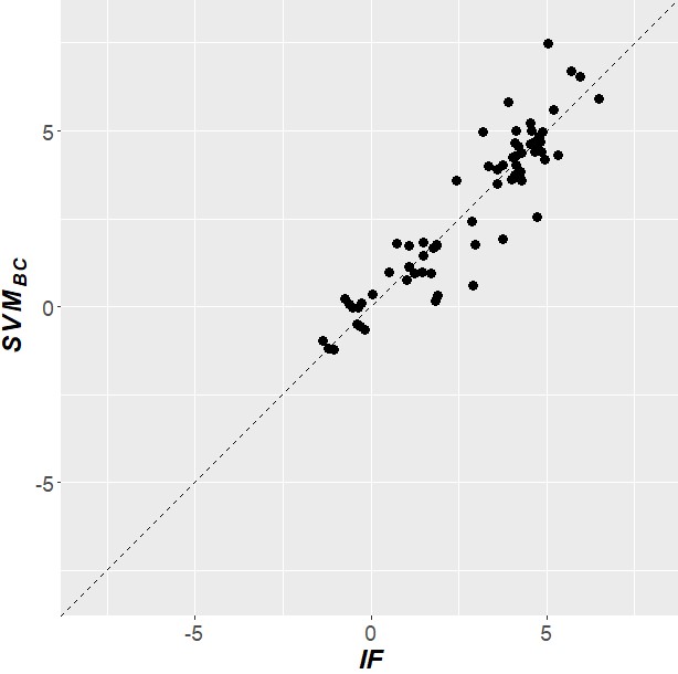
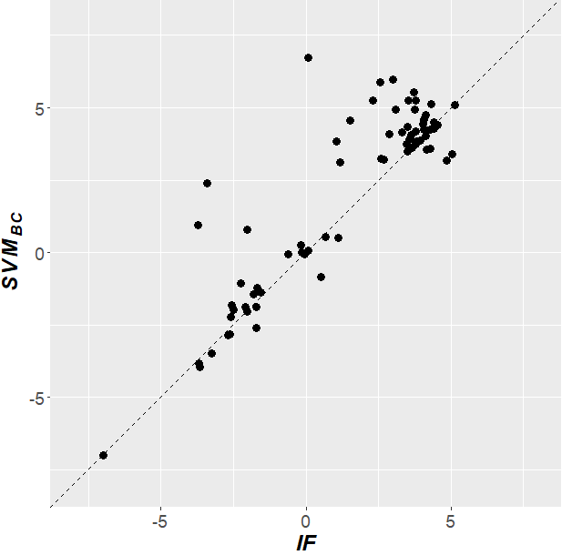
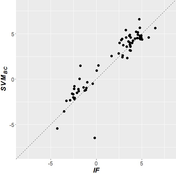
To compare the two best models, a detailed analysis between IF and grouped by the predictive models used in PMO is provided in Figure 4, in which three scatter plots comparing true optimality gap of solutions obtained from IF and (calculated as log()) are provided. Each point corresponds to an instance. A point above the dashed line at 45 degrees indicates that the true outcome of the solution obtained from IF is better than that from . When the predictive model is linear regression (Figure 4(a)), random forest (Figure 4(b)), and neural networks (Figure 4(c)), IF is better than in 36, 45, and 49 out of 70 instances, respectively.
Of note is that in Figure 4(a) we see that IF and have a similar performance when linear regression is employed as the predictive model. We hypothesize that the reason for such similar solution quality is the poor performance of linear regression in this setting (see Table 1). The performance difference between IF and is more obvious when the predictive model has higher performance. Figure 4(b) shows that with random forest as the predictive model the points tend to the bottom left corner and so are of better quality on average, but that the points deviate more from the 45 degrees dashed line in the vertical direction than in the horizontal direction, meaning that the true optimality gap from IF is much better than that from . An analogous pattern can be observed in Figure 4(c). Overall, Figure 4 clearly indicates the superiority of IF over the other tested models on the synthetic datasets. In addition, such dominance of IF can also be found in terms of the optimality error, which measures the level of overestimation at the solutions [Schweidtmann et al. 2022] and can be interpreted as the reliability of the solutions. According to Table 3, the performance of IF in terms of the optimality error is the most robust among all the models; it is the best among those models tested in 11 out of 21 scenarios. The overall improvement as compared to BASE, which is summarized in Table 2, also shows that IF is the best of all the PMO variant models.
A final takeaway is that MD and KNN are two alternative models worth exploration for any particular application. Although the performance of MD and KNN are unable to surpass SVM in terms of true outcome, both of them are better than PCA in 18 cases out of 21, and are better than CH in 9 cases and 16 cases out of 21, respectively. In addition, as summarized in Table 2, KNN ranks fourth place among the PMO variant models, only slightly worse than the best model in literature. Such good performance can also be supported by Table 3, through the results from Rastrigin in particular, which has 10 dimensions with the predictive model being linear regression and neural networks.
4.3.2 Computational Efficiency
From the results of solution outcome values reported in the Section 4.3.1, we observe that solutions from IF, SVM, and are significantly better than other PMO variant models, with IF being the best approach in terms of solution outcome quality.
Now we discuss the solution times for all models. Figure 5 shows a box plot of running time over all 10 instances using Powell as the bechmark function, with the three tested predictive models and the seven PMO variant models. Overall, Figure 5 highlights the computational efficiency of our IF model over the other models that achieve high-quality solutions based on SVMs. The running time of the majority of the instances using MD, CH, KNN, and PCA, and IF are within two seconds, but as discussed in the previous section, IF finds much better solutions. In contrast, the run time for SVM is significantly longer than other PMO variant models. For example, when the predictive model is linear regression, SVM uses nearly the full 60-minute time limit for all the 10 instances , among which only 2 instances are solved to optimality. Our implementation of improves the solution time of SVM significantly, but it still lags IF even for Powell which only has 4 dimensions.


As expected, for the functions with more dimensions, the run time performance degrades. Figure 6 summarizes the runtimes for Qing function with 8 dimensions. Despite the overall increase in run time, we see that except SVM and , the Qing instances are solved within the time limit by all the remaining models, among which, IF exhibits a robust performance regardless of the predictive model. Appendix C summarizes the run time performance over all benchmark functions, which particularly highlight the robust computational performance of IF. We should note that, for Rastrigin function, computational times across all constraint types for the random forest model are higher. This is mainly due to the instance complexities for the random forest-based PMO model even without any trust-region constraint.

4.4 Robustness Check: Sampling Away from Global Optimum
In addition to the experimental results from the 70 synthetic datasets, we also run a similar experiment on another 70 synthetic datasets by taking a different random sampling approach. To be more specific, in these datasets we exclude the samples in the neighborhood of the global optimum. With the same seven benchmark functions, we first generate 1500 sample points instead of 1000 sample points for each dataset using the same sampling procedure in Section 4.1. We then create a hole centering at the global optimum of the benchmark function with radius , where is the variance of independent variable and is obtained from the randomly generated covariance matrix. Finally, we remove sample points falling within the radius. Figure 7 illustrates the shapes of two datasets simulated using Peaks function.
Beale Peaks Griewank Powell Quintic Qing Rastrigin Linear Regression BASE 9375 11320 0.00 2.16 1.03 0.48 16121 17009 3835 7623 1992 3507 278 223 IF 11 367 -0.39 0.14 0.61 0.18 194 584 68 411 81 151 108 3 SVM 8 444 -0.85 0.10 0.96 0.23 667 251 116 1190 118 578 118 22 4 172 -0.72 0.15 0.90 0.17 603 113 102 1044 61 128 113 9 CH 581 2170 -0.02 1.35 0.92 0.20 7230 7074 3005 5008 1045 1415 142 36 PCA 1546 3184 0.00 1.07 1.04 0.42 15585 15975 5369 8206 2301 3370 267 194 MD 66 1383 -0.03 1.13 0.93 0.21 13355 13278 3770 6024 1260 1756 126 24 KNN 36 1434 -0.25 0.94 0.74 0.01 1575 1197 1552 3095 265 586 110 6 Random Forest BASE 53 627 -2.39 0.04 0.48 0.23 502 1069 250 326 254 255 84 25 IF 15 38 -1.92 0.10 0.23 0.18 115 125 95 48 54 7 60 21 SVM 80 152 -2.29 0.29 0.30 0.10 219 450 113 13 109§ 40 91§ 17 16 83 -2.63 0.64 0.26 0.14 198 377 119 16 90 72 55 12 CH 27 558 -2.42 0.02 0.46 0.20 577 1085 118 123 157 148 67 1 PCA 265 643 -4.57 2.55 0.54 0.26 842 1313 285 355 215 211 84 24 MD 154 553 -2.48 0.16 0.40 0.12 750 1261 232 252 163 158 75 16 KNN 39 536 -2.24 0.20 0.44 0.18 458 944 152 128 147 131 65 3 Neural Networks BASE 8713 9179 -0.99 5.15 1.03 1.47 5059 6742 3789 5714 2273 2802 262 190 IF 5 104 -3.76 0.59 0.18 0.03 162 291 148 204 63 155 111 12 SVM 9 133 -3.55 0.34 0.47 0.37 409 792 309 483 92 274 107§ 7 12 89 -3.66 0.47 0.38 0.27 324 653 187 504 73 226 101 1 CH 406 703 -2.53 1.35 0.40 0.36 789 1320 216 814 222 352 106 9 PCA 1038 1214 -3.88 0.65 0.94 1.04 2708 4094 2547 3851 1285 1658 228 151 MD 138 387 -2.99 0.55 0.51 0.50 911 1374 267 1012 120 291 103 12 KNN 157 407 -2.36 0.84 0.30 0.27 358 870 170 652 144 263 100 6 Best Sample 34 -1.91 0.31 334 283 158 69 § We are unable to obtain a feasible solution in 1, 7, and 3 instances out of 10 within the time limit of 60 minutes for the combinations of Qing with random forest using SVM, Rastrigin with random forest using , and Rastrigin with neural networks using , respectively.
5 Conclusions and Future Work
In this paper, we investigate seven PMO variant models with constraints describing a trust region. We assess the performance of both the constraints existing in literature and our proposed constraints, validate the importance of considering a trust region, and highlight that constraints learned from isolation forests outperform existing approaches in both solution quality and computational performance through extensive experimentation on several synthetic datasets.
Among the existing approaches, one-class SVM constraints work best in terms of solution quality but impose a high computational burden to the PMO models. In addition to isolation forest, we explore two other common outlier detection methods, Mahalanobis distance and -nearest neighbors. The performance of trust-region constraints based on these two methods is better than two other existing approaches, namely, convex hull constraints and PCA constraints.
There is a wide array of research that can expand on the work in this paper, including the following. First, we do not investigate specific algorithms well suited for each predictive model and each PMO variant model. We observed that SVM suffers from the complexity brought by the exponential constraints. Trust-region constraints in other PMO variant models could also potentially significantly increase the solution times (e.g., consider the auxiliary binary variables and big-M constraints for KNN). Advanced optimization algorithms and stronger formulations may be applicable to greatly improve computational times. Second, an investigation of which type of trust-region constraint to add for different contexts is important. We show that adding trust-region constraints nearly always leads to higher quality solutions in our experiments, but using different constraints results in varied solution quality and understanding this connection would make the decision-making pipeline more robust. Third, we explored three classes of trust-region constraints based on existing outlier detection methods. There are a variety of additional methods from the literature of outlier detection, which can be used for characterizing a trust region and could offer different tradeoffs between solution quality and computational performance.
References
- Altman [1992] Naomi S Altman. An introduction to kernel and nearest-neighbor nonparametric regression. The American Statistician, 46(3):175–185, 1992.
- Amodei et al. [2016] Dario Amodei, Chris Olah, Jacob Steinhardt, Paul Christiano, John Schulman, and Dan Mané. Concrete problems in ai safety. arXiv preprint arXiv:1606.06565, 2016.
- Anderson et al. [2020] Ross Anderson, Joey Huchette, Will Ma, Christian Tjandraatmadja, and Juan Pablo Vielma. Strong mixed-integer programming formulations for trained neural networks. Mathematical Programming, pages 1–37, 2020.
- Baardman et al. [2019] Lennart Baardman, Maxime C Cohen, Kiran Panchamgam, Georgia Perakis, and Danny Segev. Scheduling promotion vehicles to boost profits. Management Science, 65(1):50–70, 2019.
- Bergman et al. [2022] David Bergman, Teng Huang, Philip Brooks, Andrea Lodi, and Arvind U Raghunathan. Janos: an integrated predictive and prescriptive modeling framework. INFORMS Journal on Computing, 34(2):807–816, 2022.
- Bertsimas et al. [2016] Dimitris Bertsimas, Allison O’Hair, Stephen Relyea, and John Silberholz. An analytics approach to designing combination chemotherapy regimens for cancer. Management Science, 62(5):1511–1531, 2016.
- Biggs et al. [2017] Max Biggs, Rim Hariss, and Georgia Perakis. Optimizing objective functions determined from random forests. Available at SSRN 2986630, 2017.
- Biggs et al. [2021] Max Biggs, Wei Sun, and Markus Ettl. Model distillation for revenue optimization: Interpretable personalized pricing. In International Conference on Machine Learning, pages 946–956. PMLR, 2021.
- Botoeva et al. [2020] Elena Botoeva, Panagiotis Kouvaros, Jan Kronqvist, Alessio Lomuscio, and Ruth Misener. Efficient Verification of ReLU-Based Neural Networks via Dependency Analysis. Proceedings of the AAAI Conference on Artificial Intelligence, 34(04):3291–3299, April 2020. ISSN 2374-3468, 2159-5399. doi: 10.1609/aaai.v34i04.5729. URL https://aaai.org/ojs/index.php/AAAI/article/view/5729.
- Bunel et al. [2018] Rudy Bunel, Ilker Turkaslan, Philip H. S. Torr, Pushmeet Kohli, and M. Pawan Kumar. A Unified View of Piecewise Linear Neural Network Verification. arXiv:1711.00455 [cs], May 2018. URL http://arxiv.org/abs/1711.00455. arXiv: 1711.00455.
- Cheng et al. [2017] Chih-Hong Cheng, Georg Nührenberg, and Harald Ruess. Maximum resilience of artificial neural networks. In International Symposium on Automated Technology for Verification and Analysis, pages 251–268. Springer, 2017.
- Dutta et al. [2018] Souradeep Dutta, Susmit Jha, Sriram Sankaranarayanan, and Ashish Tiwari. Output range analysis for deep feedforward neural networks. In NASA Formal Methods Symposium, pages 121–138. Springer, 2018.
- Ferreira et al. [2016] Kris Johnson Ferreira, Bin Hong Alex Lee, and David Simchi-Levi. Analytics for an online retailer: Demand forecasting and price optimization. Manufacturing & Service Operations Management, 18(1):69–88, 2016.
- Fischetti and Jo [2018] Matteo Fischetti and Jason Jo. Deep neural networks and mixed integer linear optimization. Constraints, 23(3):296–309, 2018.
- Friedman [2017] Jerome H Friedman. The elements of statistical learning: Data mining, inference, and prediction. springer open, 2017.
- Gavana [2022] Andrea Gavana. Index of test functions in global optimization problems, 2022. http://infinity77.net/global_optimization/test_functions.html#multidimensional-test-functions-index, Last accessed on 2022-10-03.
- Grimstad and Andersson [2019a] Bjarne Grimstad and Henrik Andersson. Relu networks as surrogate models in mixed-integer linear programs. Computers & Chemical Engineering, 131:106580, 2019a.
- Grimstad and Andersson [2019b] Bjarne Grimstad and Henrik Andersson. ReLU networks as surrogate models in mixed-integer linear programs. Computers & Chemical Engineering, 131:106580, December 2019b. ISSN 00981354. doi: 10.1016/j.compchemeng.2019.106580.
- Gurobi Optimization LLC [2020] Gurobi Optimization LLC. Gurobi optimizer reference manual, 2020. https://www.gurobi.com.
- Hofmann et al. [2008] Thomas Hofmann, Bernhard Schölkopf, and Alexander J Smola. Kernel methods in machine learning. The annals of statistics, 36(3):1171–1220, 2008.
- Huang et al. [2019] Teng Huang, David Bergman, and Ram Gopal. Predictive and prescriptive analytics for location selection of add-on retail products. Production and Operations Management, 28(7):1858–1877, 2019.
- Johnson et al. [2014] Richard Arnold Johnson, Dean W Wichern, et al. Applied multivariate statistical analysis, volume 6. Pearson London, UK:, 2014.
- Jolliffe [2002] Ian T Jolliffe. Principal component analysis for special types of data. Springer, 2002.
- Katz et al. [2017] Guy Katz, Clark Barrett, David L Dill, Kyle Julian, and Mykel J Kochenderfer. Reluplex: An efficient smt solver for verifying deep neural networks. In International Conference on Computer Aided Verification, pages 97–117. Springer, 2017.
- Leys et al. [2018] Christophe Leys, Olivier Klein, Yves Dominicy, and Christophe Ley. Detecting multivariate outliers: Use a robust variant of the mahalanobis distance. Journal of Experimental Social Psychology, 74:150–156, 2018.
- Liu et al. [2008] Fei Tony Liu, Kai Ming Ting, and Zhi-Hua Zhou. Isolation forest. In 2008 Eighth IEEE International Conference on Data Mining, pages 413–422. IEEE, 2008.
- Liu et al. [2020] Sheng Liu, Long He, and Zuo-Jun Max Shen. On-Time Last-Mile Delivery: Order Assignment with Travel-Time Predictors. Management Science, November 2020. ISSN 0025-1909. https://pubsonline.informs.org/doi/abs/10.1287/mnsc.2020.3741.
- Lomuscio and Maganti [2017] Alessio Lomuscio and Lalit Maganti. An approach to reachability analysis for feed-forward ReLU neural networks. arXiv:1706.07351 [cs], June 2017. http://arxiv.org/abs/1706.07351,.
- Mahalanobis [1936] Prasanta Chandra Mahalanobis. On the generalized distance in statistics. National Institute of Science of India, 1936.
- Maragno et al. [2021] Donato Maragno, Holly Wiberg, Dimitris Bertsimas, S Ilker Birbil, Dick den Hertog, and Adejuyigbe Fajemisin. Mixed-integer optimization with constraint learning. arXiv preprint arXiv:2111.04469, 2021.
- Mišić [2020] Velibor V Mišić. Optimization of tree ensembles. Operations Research, 68(5):1605–1624, 2020.
- Mistry et al. [2021] Miten Mistry, Dimitrios Letsios, Gerhard Krennrich, Robert M Lee, and Ruth Misener. Mixed-integer convex nonlinear optimization with gradient-boosted trees embedded. INFORMS Journal on Computing, 33(3):1103–1119, 2021.
- Papageorgiou [2020] Ioulia Papageorgiou. Ceramic investigation: how to perform statistical analyses. Archaeological and Anthropological Sciences, 12(9):1–19, 2020.
- Pedregosa et al. [2011] F. Pedregosa, G. Varoquaux, A. Gramfort, V. Michel, B. Thirion, O. Grisel, M. Blondel, P. Prettenhofer, R. Weiss, V. Dubourg, J. Vanderplas, A. Passos, D. Cournapeau, M. Brucher, M. Perrot, and E. Duchesnay. Scikit-learn: Machine learning in Python. Journal of Machine Learning Research, 12:2825–2830, 2011.
- Sahinidis [2017] N. V. Sahinidis. BARON 21.1.13: Global Optimization of Mixed-Integer Nonlinear Programs, User’s Manual, 2017.
- Schölkopf et al. [1999] Bernhard Schölkopf, Robert C Williamson, Alex Smola, John Shawe-Taylor, and John Platt. Support vector method for novelty detection. Advances in neural information processing systems, 12, 1999.
- Schweidtmann and Mitsos [2019] Artur M Schweidtmann and Alexander Mitsos. Deterministic global optimization with artificial neural networks embedded. Journal of Optimization Theory and Applications, 180(3):925–948, 2019.
- Schweidtmann et al. [2022] Artur M Schweidtmann, Jana M Weber, Christian Wende, Linus Netze, and Alexander Mitsos. Obey validity limits of data-driven models through topological data analysis and one-class classification. Optimization and Engineering, 23(2):855–876, 2022.
- Serra et al. [2018] Thiago Serra, Christian Tjandraatmadja, and Srikumar Ramalingam. Bounding and counting linear regions of deep neural networks. In International Conference on Machine Learning, pages 4558–4566. PMLR, 2018.
- Tax [2001] DMJ Tax. One class classification: Concept learning in the absence of counter examples [ph. d dissertation]. Netherlands Delft University of Technology. Faculty of Information Technologand Systems, 2001.
- Teixeira et al. [2006] Ana P Teixeira, João J Clemente, António E Cunha, Manuel JT Carrondo, and Rui Oliveira. Bioprocess iterative batch-to-batch optimization based on hybrid parametric/nonparametric models. Biotechnology progress, 22(1):247–258, 2006.
- The MathWorks Inc [2010] The MathWorks Inc. peaks minimization with globalsearch, 2010. https://www.mathworks.com/matlabcentral/mlc-downloads/downloads/submissions/27178/versions/6/previews/html/gsPeaksExample.html, Last accessed on 2022-10-03.
- Tjeng et al. [2019] Vincent Tjeng, Kai Xiao, and Russ Tedrake. Evaluating Robustness of Neural Networks with Mixed Integer Programming. arXiv:1711.07356 [cs], February 2019. http://arxiv.org/abs/1711.07356.
- Tsay et al. [2021] Calvin Tsay, Jan Kronqvist, Alexander Thebelt, and Ruth Misener. Partition-based formulations for mixed-integer optimization of trained relu neural networks. arXiv preprint arXiv:2102.04373, 2021.
- Verwer et al. [2017] Sicco Verwer, Yingqian Zhang, and Qing Chuan Ye. Auction optimization using regression trees and linear models as integer programs. Artificial Intelligence, 244:368–395, 2017.
- Wang et al. [2021] Keliang Wang, Leonardo Lozano, David Bergman, and Carlos Cardonha. A two-stage exact algorithm for optimization of neural network ensemble. In International Conference on Integration of Constraint Programming, Artificial Intelligence, and Operations Research, pages 106–114. Springer, 2021.
- Zheng et al. [2021] Shuo Zheng, Yu-Xin Zhu, Dian-Qing Li, Zi-Jun Cao, Qin-Xuan Deng, and Kok-Kwang Phoon. Probabilistic outlier detection for sparse multivariate geotechnical site investigation data using bayesian learning. Geoscience Frontiers, 12(1):425–439, 2021.
Appendix A PMO Formulations with Different Predictive Models
A.1 Linear Regression-based PMO Formulation
For a linear regression model, the objective function can be expressed as . As a result, the PMO formulation is given by the following linear program:
| (A.1a) | ||||
| s.t. | (A.1b) | |||
A.2 Random Forest-based PMO Formulation
A.2.1 Background on Random Forests
We consider random forest regression models in this paper, where the outcome variable is continuous. Let be the index set of trees in the random forest. Each tree has the same weight in the prediction and is trained over a randomly selected subsample of the training data. Similar to isolation trees, the prediction for an observation is determined by checking a series of splits. Each leaf node from tree has a score . Any vector of independent variables corresponds to a leaf node of the tree, denoted by . The predicted outcome for an input vector from tree is given by the corresponding score . As a result, the prediction of the random forest for a given is given by the average of the corresponding scores:
A.2.2 Optimization Model
Inspired by Mišić 2020, we present a PMO formulation to solve optimization problems over a pre-trained random forest. The objective of the optimization problem is to find the independent variable vector that minimizes the outcome predicted by the random forest . This can be casted as the problem of finding a leaf node from each tree in the random forest that minimize the average outcome.
Consider a random forest with trees. Let be the set of leaf nodes in tree . We introduce binary decision variable that takes a value of 1 if leaf node from tree is selected. We introduce auxiliary decision variables () to specify the range of each variable feature . Let the lower and upper bounds corresponding to a leaf node be and for all . Our formulation of the random forest-based optimization problem is:
| (A.2a) | |||||
| s.t. | (A.2b) | ||||
| (A.2c) | |||||
| (A.2d) | |||||
| (A.2e) | |||||
| (A.2f) | |||||
| (A.2g) | |||||
Constraints (A.2b) ensure that exactly one of the leaf nodes from each tree in the random forest is selected. Constraints (A.2c) and constraints (A.2d) ensure that, for any leaf node that is selected, the domain of the solution is limited to the feature ranges determined by the path leading to that leaf node. Constraints (A.2e) ensure that belongs to the domain defined by the corresponding leaf nodes selected.
A.3 Neural Networks-based PMO Formulation
There is plenty of literature on formulating neural networks models as a mixed integer programming problem. In particular, we make use of recent work that solve the neural networks-based optimization problem. For the details of the formulation, the reader is refered to Bergman et al. 2022.
Appendix B Details of the Branch-and-Cut Algorithm for PMO Model with One-Class SVM Constraints
Recall that are the main decision variables in a PMO model, determining the value of each feature . For the branch-and-cut algorithm, we first discretize the range of each feature into m pieces. As each feature is scaled to [0,1], the pieces of the discretized ranges for each feature are , where is a small number (we set ). Binary decision variable equals 1, if the value of feature falls into range . The master problem is formulated on the basis of PMO model (1a) with additional constraints connecting decision variables and :
| (B.1) | |||||
| (B.2) | |||||
| (B.3) | |||||
| (B.4) | |||||
We describe the procedure of our proposed branch-and-cut algorithm in Algorithm 1 and note that this branch-and-cut algorithm is a heuristic. The algorithm can be implemented using a call-back function by dynamically checking sub-problem constraints for integer nodes, and adding cuts while the branch-and-bound tree is being built.
Note that the cover cuts ensure that any given combination of the discretization ranges is explored at most once during the execution of the algorithm. The algorithm terminates in a finite number of steps because there is a finite number of combinations for the discretization ranges.
Appendix C Running Time Summary of Each Benchmark Function


