A Mirage or an Oasis? Water Vapor in the Atmosphere of the Warm Neptune TOI-674 bFacilities: HST, TESS, Spitzer, MAST, ExoFOP, Exoplanet Archiveastropy (Astropy Collaboration et al. 2013; Astropy Collaboration et al. 2018), ExoCTK (Bourque et al. 2021), exoplanet (Foreman-Mackey et al. 2021), starry (Luger et al. 2019), petitRADTRANS (Mollière et al. 2019; Mollière et al. 2020), Iraclis (Tsiaras et al. 2016a; Tsiaras et al. 2016b; Tsiaras et al. 2018)
Abstract
We report observations of the recently discovered warm Neptune TOI-674 b (5.25 , 23.6 ) with the Hubble Space Telescope’s Wide Field Camera 3 instrument. TOI-674 b is in the Neptune desert, an observed paucity of Neptune-size exoplanets at short orbital periods. Planets in the desert are thought to have complex evolutionary histories due to photoevaporative mass loss or orbital migration, making identifying the constituents of their atmospheres critical to understanding their origins. We obtained near-infrared transmission spectroscopy of the planet’s atmosphere with the G141 grism. After extracting, detrending, and fitting the spectral lightcurves to measure the planet’s transmission spectrum, we used the petitRADTRANS atmospheric spectral synthesis code to perform retrievals on the planet’s atmosphere to identify which absorbers are present. These results show moderate evidence for increased absorption at 1.4 m due to water vapor at 2.9 (Bayes factor = 15.8), as well as weak evidence for the presence of clouds at 2.2 (Bayes factor = 4.0). TOI-674 b is a strong candidate for further study to refine the water abundance, which is poorly constrained by our data. We also incorporated new TESS short-cadence optical photometry, as well as Spitzer/IRAC data, and re-fit the transit parameters for the planet. We find the planet to have the following transit parameters: , BJD, and d. These measurements refine the planet radius estimate and improve the orbital ephemerides for future transit spectroscopy observations of this highly intriguing warm Neptune.
Keywords:
Exoplanet atmospheres (487) — Exoplanet atmospheric composition (2021) — Transmission spectroscopy (2133) — M stars (985) — Near infrared astronomy (1093) — Hubble Space Telescope (761)I Introduction
The last two and a half decades of exoplanet science have revealed a wealth of information on planetary system architectures. The first discovered exoplanet around a main-sequence star star, 51 Pegasi b (Mayor & Queloz 1995) is a Hot Jupiter, one of a class of planets that challenged our ideas on the formation and evolution of planetary systems. As the field has progressed, these astonishing outliers have proven to be representative of larger planetary populations in systems often unlike our own.
In addition to these populations, several gaps in the distribution of short-period exoplanets have also been noted, namely the radius valley (Fulton et al. 2017) and the Neptune desert (Mazeh et al. 2016). For the radius valley, atmospheric mass loss due to host star irradiation is the main theory for the observed lack of 1.5–2 planets at these short orbital periods (Owen & Wu 2017). Other explanations due to formation mechanisms and core-powered mass loss (Ginzburg et al. 2018) have also been put forth, as well as a primordial radius gap due to late gas accretion in gas-poor nebulae (Lee & Connors 2021). The Neptune desert is a similar lack of planets at even shorter orbital periods ( d) but for approximately Neptune-to-Jupiter mass planets (Mazeh et al. 2016). The lower-mass section of the gap may be appropriately explained by irradiative atmospheric stripping, but the dearth of Jupiter-mass planets in this narrow period range may be better explained by planetary migration and in-situ formation (Owen & Lai 2018; Bailey & Batygin 2018).
The Neptune desert is especially relevant, given the uncertainties in our own solar system about the formation of Uranus and Neptune, either through core accretion (Frelikh & Murray-Clay 2017) or disk instability (Boss 2003). We presume migration processes were important in their early histories as they would have been for Jupiter and Saturn, and by proxy also the observed exoplanetary populations. Transit surveys are not generally sensitive to these cold giant planets, and efforts to measure the true frequency of Solar system analogs rely on long-baseline radial velocity surveys (Wittenmyer et al. 2020). However, these surveys still do not have the time baselines or RV precision to detect Uranus and Neptune-like planets, which would require m/s RV precision, aided by as astrometry from Gaia (Wittenmyer et al. 2020).
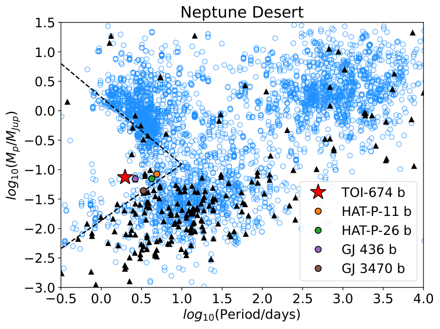
As can be seen in Fig. 1, fewer total planets with measured masses are known to orbit M-dwarfs than other stellar types, making it difficult to say with certainty whether the Neptune desert exists around the coolest stars. As the upper boundary of the Neptune desert is characterized by planets with masses , the upper bound for the M-dwarf Neptune desert is unclear given the general lack of massive planets around M-dwarfs. However, the lower boundary of the desert appears to hold for the M-dwarf planet population.
It is especially tempting to want to characterize the few large planets known to exist in the desert. Several high profile planet discoveries have been made in the Neptune desert (Bakos et al. 2010; Borucki et al. 2010; Hartman et al. 2011; Bonomo et al. 2014; Bakos et al. 2015; Crossfield et al. 2016; Eigmüller et al. 2017; Barragán et al. 2018; West et al. 2019; Jenkins et al. 2020), and these planets may be exceptional in several ways. Young Neptune desert planets may be undergoing atmospheric mass loss, or may be in the process of migrating into the desert. Older Neptune desert planets may have already lost parts of their atmospheres, or finished their migrations. However, as this is only a relatively recently identified population, only a few have been characterized by atmospheric transmission spectroscopy (GJ 436 b: Knutson et al. 2014a, HAT-P-26 b: Wakeford et al. 2017, GJ 3470 b: Benneke et al. 2019, HAT-P-11 b: Chachan et al. 2019). These atmospheres range from featureless (GJ 436 b) to strongly featured (HAT-P-26 b), and also have varying metallicity, with both low metallicities (HAT-P-11 b, HAT-P-26 b and GJ 3470 b) and ambiguous metallicities (GJ 436 b), where both high and low metallicities could produce the observed atmosphere. Here we present Hubble Space Telescope (HST) Wide Field Camera 3 (WFC3) infrared (IR) spectroscopic observations of the recently discovered warm Neptune TOI-674 b.
I.1 TOI-674 b
The TESS observatory recently discovered TOI-674 b, a warm Neptune (5.25 , 23.6 ) orbiting a nearby M2 dwarf (TIC 158588995, V=14.2 mag, J=10.4 mag, RA 105820.98 DEC -36∘51′29.13′′ (J2000), 46.16 pc, 0.420 , 0.420 ) with a period of 1.977143 days (Murgas et al. 2021). With these parameters, TOI-674 b is in the Neptune desert (see Fig. 1), experiencing 38 times as much stellar radiation as the Earth does (Murgas et al. 2021).
TOI-674 b also provides a good target for atmospheric transmission spectroscopy, which attracted our attention during the first year of the TESS mission. Given the small size of the host star and relatively large radius of the planet, TOI-674 b has a high transmission spectroscopy metric of 222 (see Kempton et al. 2018 for a definition of this quantity). Compared to other similar planets in the desert (Murgas et al. 2021, see e.g. Fig. 10 in ), these factors make it one of the best planets of its class for transmission spectroscopy.
In Section II, we describe our data and analyses, including details of our transit and systematics models for the HST WFC3 data, as well as the TESS and Spitzer data. In Section III, we present the details and results of the atmospheric retrieval framework used here, and in Section IV, we discuss the implications of these results, including future observations.
II Data, Data Reduction, and Analysis
II.1 Observations
We observed three transits of TOI-674 b on 10, 12, and 26 July 2020 with the Hubble Space Telescope’s (HST) Wide Field Camera 3 instrument, as part of the large HST General Observer Program 15333 (Co-PIs: Crossfield and Kreidberg). Each transit visit consisted of four orbits, and each orbit started with one direct image in the F130N filter, and then continued with spectroscopic imaging with the G141 grism (m – m). 55 exposures were taken in Visit 1, 60 exposures were taken in Visit 2, and 52 exposures were taken in Visit 3. All spectral exposures were taken with round-trip spatial scanning (McCullough & MacKenty 2012; Deming et al. 2013), and each scan direction had an exposure time of 134 seconds. The scan rate was 0.043 arcsec/s, and the scan length was 6.08 arcsec. All HST data analyzed in this paper can be found in MAST at: http://dx.doi.org/10.17909/tvy9-7h80 (catalog 10.17909/tvy9-7h80).
As TOI-674 b was discovered by the Transiting Exoplanet Survey Satellite (TESS) (Ricker et al. 2015), we also have access to planet transit data in the TESS bandpass. The discovery paper was based on 22 transits observed in TESS Sectors 9 and 10 (Murgas et al. 2021), and we use new photometry of the planet consisting of 11 transits in TESS Sector 36. Finally, we also observed a single transit of TOI-674 b with the Spitzer Space Telescope’s IRAC instrument in the m channel (also incorporated into (Murgas et al. 2021)) Further discussion of these observations is presented in Section II.2.3. We incorporate both the TESS and Spitzer transit depths into our eventual atmospheric retrievals (see Sec. III).
II.2 Data Reduction and Analysis
We used the Iraclis pipeline (Tsiaras et al. 2016a; Tsiaras et al. 2016b; Tsiaras et al. 2018) to reduce the raw spatially scanned HST data and extract spectral lightcurves. Iraclis performs a standard set of HST WFC3 image reduction steps (e.g. calibrating, flat-fielding, bad pixel/cosmic ray correction, etc.) and then extracts the spectrum from the reduced images.A full description of the Iraclis reduction steps are given in Tsiaras et al. 2016a; Tsiaras et al. 2016b; Tsiaras et al. 2018. Iraclis ingests HST flat-fielded direct images of the target star to locate the target on the detector, and then extracts the spatially scanned spectrum from the raw spectral data files. After conducting the reduction and extraction, Iraclis returns the reduced images and extracted spectra, along with some diagnostic information. Input parameter files allow a user to modify various aspects of the reduction, extraction, and fitting process. In order to determine the optimal extraction aperture to minimize scatter in the spectrophotometric lightcurves, we ran Iraclis with varying extraction apertures from 0 pixels above and below the spectrum to 20 pixels above and below the spectrum in 5 pixel increments. We then fit the broadband lightcurves for each extraction aperture and logged the RMS error for each. The 10 pixel aperture yielded the lowest RMS error, and we used this aperture for our extraction. We extracted 18 spectral bins ranging from m to m, such that each bin contains approximately equal stellar flux. The extracted lightcurves were then used as inputs for our transit model and systematics fitting process.
II.2.1 Transit and Systematics Models
HST/WFC3 lightcurves offer precise transit measurements but are known to be subject to significant systematic effects. In order to detrend the transit lightcurves we modified the model-ramp method from Kreidberg et al. 2014 to fit our data. Our modification of the model-ramp method fits the systematics and the transit parameters simultaneously as follows:
| (1) | ||||
is the full model to the observed data, is the out-of-transit mean flux, is the bare normalized transit lightcurve, is a visit-long slope, is the amplitude of the ramp systematic, is the ramp systematic timescale, is a vector of the times elapsed since the first exposure in the current visit, the amplitude of the scan-direction sinusoid, a vector of the times elapsed since the first exposure in the current orbit, and the average duration between the start of each exposure. are subscripts denoting spectral bin central wavelength, HST visit, and orbit number. We also include an extra error term , added in quadrature to the per-integration flux uncertainty, which we find aids in sampling.
Following previous analyses (Deming et al. 2013; Wakeford et al. 2016; Zhou et al. 2017; Alderson et al. 2022), we discard the initial orbit in each visit due to the strong effect of the ramp systematic in that orbit, and we also found that the initial spectral exposure in each orbit was also strongly affected by the ramp systematic and discarded it as well. Using the exoplanet toolkit (Foreman-Mackey et al. 2021), we fit the white-light transit lightcurves for each transit, fitting the exponential orbit-level ramp and visit-long slope systematics models as described in Kreidberg et al. 2014, and correcting for the round-trip scan effect with a sinusoidal model. We describe our method for correcting the spatial scan systematic in more detail in Appendix A, as well as benchmark it against legacy methods. The transit lightcurve and systematics parameters are normalized such that the out of transit flux is 1, and then the entire model is multiplied by the mean out of transit flux observed in the HST data.
Our HST transit model incorporated the published star and planet parameters from Murgas et al. 2021, except where those parameters were refined by our new fit to the TESS data incorporating Sector 36. The stellar and planetary parameter priors are shown in Table 1. Limb darkening coefficients for the broadband transit and spectral bins were pre-calculated using the Limb Darkening Calculator in the Exoplanet Characterization Toolkit (ExoCTK) (Bourque et al. 2021), using the published stellar parameters from Murgas et al. 2021, and the Kurucz ATLAS9 stellar models. All parameter estimation was conducted with the exoplanet toolkit (Foreman-Mackey et al. 2021), built on top of PyMC3 (Salvatier et al. 2016) for posterior sampling. exoplanet uses gradient-based inference methods to improve sampling performance compared to ensemble samplers or nested sampling, which are more commonly used in astronomy. Here we use exoplanet’s No U-Turn Sampler (Hoffman & Gelman 2011) implementation. exoplanet also allows for the simulation of transit lightcurves using starry (Luger et al. 2019). For each of the HST transit fits (the white lightcurve and each spectral lightcurve, for each visit), we ran 4 chains for 2000 tuning steps (analogous to traditional MCMC burn-in, but the sampler adjusts the step sizes to better fit the gradient of the log-probability of instead of hopefully exiting a bad starting point) and then drew 4000 samples from which to construct our posterior distributions.
For the first transit observed, an example white-light transit fit can be seen in Figure 2. The white-light fits for transits 2 and 3 can be found in Appendix B.
| Parameter | Prior | |
|---|---|---|
| (BJD) | ||
| Lognormal(ln(0.1135), ln(0.001)) | ||
| (d) | 1.977198 | |
| 0.0 | ||
| 0.0 | ||
| Lognormal(, ln()) | ||
| LogNormal(, 1.0) | ||
| InverseGamma(1800, 100) |
Note. — Transit parameters used for the fitting priors were taken from our re-analysis of the full TESS transit dataset of TOI-674 b. The prior on was chosen by eye to correspond with the first HST transit. Rows marked with * denote fixed values in the transit fit. is the mean out-of-transit flux, is , and is the duration of the first visit.
After modeling the WFC3 broadband transit lightcurves, we fit each of the spectral lightcurves individually, yielding the full transit spectrum. Specifically, we fixed the transit parameters to the fit white-lightcurve values except for , and re-fit the systematics parameters with the priors described in Table 1. We re-fit the systematics parameters as we noticed that they tended to be dependent on wavelength, especially in the case of the round-trip scanning flux offset. We also checked our transits for correlated noise by binning the data between 1 and 20 points and calculating the rms for each bin size. Fig. 5 shows the RMS trend deviation for each spectral lightcurve bin in each visit. The expected trend due to uncorrelated noise is , and our measured RMS error generally follows the uncorrelated noise trend, even though the bin sizes are relatively small. After fitting each visit, we averaged the spectra together in order to obtain the full transmission spectrum of the planet. The detrended and fitted lightcurves for transit 1 are shown in Figure 3. The detrended and fitted lightcurved for transits 2 and 3 are shown in B. The measured transit depths and their uncertainties are shown in Table 2. Fig. 4 shows the final averaged spectrum from TOI-674 b, as well as the individual spectra for each HST visit. Visit 3 has notably higher transit depth between m and m, but shows no evidence of starspot/facula crossings during the transit nor evidence of badly corrected cosmic ray hits in the data. This is seen as a consistent flux increase of electrons in Visit 3 compared to Visits 1 and 2. The rotation period of the star is comparable to the interval between the second and third visit, and while stellar variability may possibly be the culprit, there is no evidence in the broadband or spectral lightcurves to indicate this in any more detail.
| Wavelength | Depth | Error | ||
|---|---|---|---|---|
| () | (ppm) | (ppm) | (fixed) | (fixed) |
| TESS Depth | ||||
| 0.591 – 0.992 | 12900 | 169 | 0.098 | 0.248 |
| HST Depths | ||||
| 1.111 – 1.142 | 13078 | 115 | 0.133 | 0.212 |
| 1.142 – 1.171 | 12963 | 113 | 0.132 | 0.212 |
| 1.171 – 1.199 | 13061 | 110 | 0.128 | 0.207 |
| 1.199 – 1.226 | 13083 | 110 | 0.129 | 0.206 |
| 1.226 – 1.252 | 13128 | 106 | 0.126 | 0.202 |
| 1.252 – 1.279 | 13093 | 105 | 0.123 | 0.198 |
| 1.279 – 1.306 | 12956 | 104 | 0.128 | 0.198 |
| 1.306 – 1.332 | 13078 | 104 | 0.118 | 0.195 |
| 1.332 – 1.359 | 13306 | 103 | 0.118 | 0.209 |
| 1.359 – 1.386 | 13310 | 103 | 0.118 | 0.208 |
| 1.386 – 1.414 | 13172 | 102 | 0.120 | 0.225 |
| 1.414 – 1.442 | 13292 | 101 | 0.122 | 0.227 |
| 1.442 – 1.472 | 13211 | 100 | 0.120 | 0.232 |
| 1.472 – 1.503 | 13174 | 99 | 0.121 | 0.230 |
| 1.503 – 1.534 | 13143 | 97 | 0.112 | 0.234 |
| 1.534 – 1.568 | 13159 | 97 | 0.110 | 0.242 |
| 1.568 – 1.604 | 13015 | 94 | 0.111 | 0.245 |
| 1.604 – 1.643 | 13132 | 93 | 0.095 | 0.228 |
| Spitzer Depth | ||||
| 3.998 – 5.007 | 13317 | 1800 | 0.041 | 0.170 |

II.2.2 Independent Analysis
In addition to our method, we also used Iraclis’s transmission spectroscopy modeling capabilities to conduct an independent analysis of the data. Iraclis also fits individual HST visits, and uses the divide-white method as described in Kreidberg et al. 2014. Again, we took the unweighted average of the individual visits to obtain the transmission spectrum for our entire dataset. We found that the Iraclis results were consistent with our own analysis to within , which validates our modeling approach.
II.2.3 Spitzer and TESS Data Points
TOI-674 b was originally observed in TESS Sectors 9 and 10. The discovery paper included data from these two sectors, but TOI-674 b was also observed in TESS Sector 36, from 2021 March 7, to 2021 April 1. We re-fit the TESS data including the new sector of data in order to refine the observed and derived transit parameters, including a search for transit timing variations (TTVs) that could show evidence of undiscovered companions to TOI-674 b. Using the exoplanet toolkit, we fit the planet’s transit parameters (, , , , , , , and ) as well as the mean out-of-transit flux, fixing the stellar limb-darkening parameters to the values from Murgas et al. 2021, and fixing the orbital eccentricity to 0. exoplanet includes limb-darkened lightcurve models from starry, and since there were no strong systematics or stellar variability in the TESS lightcurve, our transit model was fairly simple:
where is the out-of-transit mean flux, and is the bare transit lightcurve. The full fit TESS lightcurve is shown in Figure 6, and folded transit data is shown in Fig. 7. exoplanet also includes the ability to fit for TTVs by simply fitting the individual transit times of an otherwise Keplerian planetary orbit. By subtracting the transit time as predicted from a linear ephemeris from each fit transit time, we retrieve the TTVs of the lightcurve. More details are available in the exoplanet documentation11 1 https://gallery.exoplanet.codes/tutorials/ttv/. Including the Sector 36 data, we found BJD and d. The full results of the transit analysis are shown in Table 3, and the TTVs are shown in Figure 8. The O-C diagram shows that the transit times are consistent with a linear ephemeris, in agreement with the analysis performed in the original discovery paper. Even without a detection of a new planet in the system, the refined transit parameters and ephemerides will be useful for further studies of this planet.

Also, as reported in the discovery paper, a single transit of TOI-674 b was observed by the Spitzer Space Telescope on 2019 September 29 as part of a program dedicated to IRAC follow-up of TESS planet candidates (GO-14084, PI: Crossfield). TOI-674 b was observed at m using Spitzer’s IRAC instrument (Fazio et al. 2004). Using the updated parameters from the full TESS transit fit as priors, we reanalyzed the archival Spitzer data. Both the TESS and Spitzer transit fit results are shown in Table 3. We incorporate the TESS and Spitzer transit depths into our observed WFC3 spectrum for the purposes of our later atmospheric retrievals as seen in Table 2.
To extract photometry from the Spitzer observations, we used the Photometry for Orbits Eclipses and Transits (POET 22 2 https://github.com/kevin218/POET) package (Cubillos et al. 2013; May & Stevenson 2020). With POET, we created a bad pixel mask and discarded bad pixels based on the Spitzer Basic Calibrated Data (BCD). We ran two iterations of sigma-clipping at the level to discard outlier pixels. We determined the center of the point spread function (PSF) is using a 2-D Gaussian fitting technique and, extracted the lightcurve using aperture photometry in combination with a BiLinearly-Interpolated Subpixel Sensitivity (BLISS) map described in Stevenson et al. 2012. We fit the resulting lightcurve with a model that accounts for both the lightcurve itself and a temporal ramp-like trend attributed to charge trapping. Finally, we sampled the posterior distributions using POET’s MCMC implementation with chains initialized at the best fit values.
We performed aperture photometry with various aperture sizes (ranging from 2–6 pixels in increments of 1 pixel). We found the optimal aperture size to be 3 pixels as this size returned the lowest standard deviation of the normalized residuals (SDNR). We then tested bin sizes of 0.1, 0.03, 0.01, and 0.003 square pixels for the BLISS map, and found that a bin size of 0.03 sq px minimized the SDNR. We generated the model lightcurve using the batman package (Kreidberg 2015) with , , and as free parameters, as well as our sysematics model, a ramp-based model with a constant offset term. We held quadratic limb darkening terms constant to those found by averaging the values found by Claret & Bloemen 2011 for , , and metallicity of 0.0. We initialized four chains sampled until convergence with 10,000 burn-in steps. The resulting transit parameters are shown in Table 3.
| Parameter | Value | Error |
|---|---|---|
| TESS Observed Parameters | ||
| (BJD) | 2458544.523792 | 0.000452 |
| P (d) | 1.977198 | 0.00007 |
| 0.1135 | 0.0006 | |
| b | 0.682 | 0.006 |
| TESS Derived Parameters | ||
| a (AU) | 0.0231 | 0.0000003 |
| 11.821 | 0.0002 | |
| i (deg) | 86.69 | 0.03 |
| () | 5.20 | 0.030 |
| Spitzer Observed Parameters | ||
| (BJD) | 2458756.0796 | 0.00012 |
| 0.1154 | 0.0009 | |
| b | 0.651 | 0.063 |
| Spitzer Derived Parameters | ||
| a (AU) | 0.0243 | 0.0012 |
| 12.44 | 0.46 | |
| i (deg) | 87.00 | 0.27 |
| () | 5.29 | 0.17 |
| Spitzer Quad. Limb Darkening | ||
| 0.0412 | ||
| 0.170 |
Note. — Parameters without stated ranges were fixed in the transit fit.
III Atmospheric Retrievals
III.1 petitRADTRANS
We used petitRADTRANS (pRT), an open-source atmospheric spectral synthesis package (Mollière et al. 2019; Mollière et al. 2020) to conduct our atmospheric retrievals. petitRADTRANS can be combined with several sampling packages to conduct atmospheric retrievals, and we used the suggested configuration by combining it with PyMultiNest (Buchner et al. 2014), a Python-based implementation of the MultiNest nested sampling code (Feroz et al. 2009).
In order to determine what molecules might be present in TOI-674 b’s atmosphere, we conducted free chemistry retrievals for the abundances of specific atmospheric species, namely , , , and (Chubb et al. 2021, all from ExoMol:), and CO (Rothman et al. 2010, from HITEMP:) following previous observational (Benneke & Seager 2013), and theoretical work (Miller-Ricci et al. 2009), as these are some of the dominant opacity sources in the NIR. We also fit for the presence or absence of clouds, here represented as a uniform opaque gray cloud at a specific atmospheric pressure. The full model incorporating all of the absorbers is compared to models removing one absorber at a time, and if the model without that absorber is less favored than the full model, we can say that the absorber is likely present. Prior distributions for our retrievals are shown in Table 4.
| Parameter | Prior | |
|---|---|---|
| log(g) log | ||
| T (K) | ||
| log(Pcloud) log(bar) | ||
| log(mass frac) | ||
| log(mass frac) | ||
| CO log(mass frac) | ||
| log(mass frac) | ||
| log(mass frac) | ||
We fixed the stellar radius, set uniform priors on the planet’s radius, and temperature, and log-uniform priors on the planet’s gravity, mass fraction of each absorber, and the cloudtop pressure. The retrievals were conducted using isothermal atmospheric models to create the planet spectra. Without proper bounds on the planetary temperature, the atmospheric retrievals may find non-physical temperatures for this planet. In order to avoid this, we bound the temperature prior with some reasonable assumptions. The equilibrium temperature of a planet can be estimated either with or without incorporating heat redistribution:
Or:
Where is a measure of heat redistribution in the range (Seager 2010). Without incorporating heat redistribution, and assuming a planetary albedo of 0.3, Murgas et al. 2021 estimated the equilibrium temperature of the planet to be K. Assuming an albedo range of , including the extreme bounds of heat redistribution, and for the stellar K, we calculate that the planet K.
All atmospheric models were created at a resolution of 1000, and we ran Multinest to completion with 1000 live points at a sampling efficiency of 80%. Each retrieval has an associated Bayesian evidence value , and the ratio of two evidences gives the Bayes factor :
where is the model evidence for the full model, and is the model evidence for a particular retrieval missing an absorber. Following Trotta 2008, Bayes factors can be converted to p-values, and then standard deviations, by the formulas:
where is the Bayes factor and the p-value, and:
where is the sigma significance and erf is the error function. Trotta 2008 and Benneke & Seager 2013 present ranges of Bayes factors that correspond to p-values and sigma significances, with () a “weak detection”, () a “moderate detection”, and () a “strong detection”. The Bayes factor analysis results are shown in Table 5. We find that the presence of is moderately favored with a Bayes factor of 15.8, corresponding to a detection, and we find weak evidence for the presence of clouds at a Bayes factor of 4.0 (), but the evidence for the other absorbers is insignificant. We also present the best-fit values for the full model in Table 6, and the 2-D posterior distributions in Figure 9.

III.1.1 Utility of Equilibrium Chemistry Models
Previous theoretical (Moses et al. 2013) work on Neptune-sized exoplanets has revealed a diversity of potential atmospheric compositions ranging from “typical” hydrogen/helium dominated atmospheres to “exotic” atmospheres dominated by significantly heavier gases such as and . Observationally, warm Neptune atmospheres range from clear (Fraine et al. 2014, HAT-P-11 b:) to cloudy (Knutson et al. 2014b, GJ 436 b:), and low-metallicity (Benneke et al. 2019, HAT-P-26 b:) to high-metallicity (Wakeford et al. 2017; Morley et al. 2017, GJ 3470 b and GJ 436 b:). We compared our observed spectra to self-consistent atmospheric models (interpolated chemical abundances based on nonequilibrium chemistry in the easyCHEM grid described in Mollière et al. 2017) and found that our data are not precise enough, nor do they have the wavelength coverage to distinguish between high-metallicity clear models and low-metallicity cloudy models (as seen in Figure 11). Future observations with JWST would provide both better precision as well as sensitivity across wider bandpasses, allowing future investigators to study the equilibrium chemistry of this planet further.
| Retrieval Model | DOF | BIC | Bayes Factor for | ||||
|---|---|---|---|---|---|---|---|
| molecule present | |||||||
| Full Model | |||||||
| H2O, CH4, CO, CO2, NH3, Cloudy | 11 | 7.5 | 0.7 | 34.4 | -5.5 | 0.0 | 1.0 |
| No H2O | 12 | 15.1 | 1.3 | 39.1 | -6.7 | 1.2 | 15.8 |
| No Cloud | 12 | 9.0 | 0.8 | 33.0 | -6.1 | 0.6 | 4.0 |
| No CO2 | 12 | 6.5 | 0.5 | 30.5 | -5.3 | -0.2 | 0.6 |
| No NH3 | 12 | 8.1 | 0.7 | 32.1 | -5.3 | -0.2 | 0.6 |
| No CO | 12 | 7.3 | 0.6 | 31.3 | -5.3 | -0.2 | 0.6 |
| No CH4 | 12 | 6.7 | 0.6 | 30.7 | -5.2 | -0.3 | 0.5 |
| Featureless | 16 | 18.8 | 1.6 | 42.8 | -6.1 | 0.6 | 4.0 |
| Constant-Depth | 19 | 20.1 | 1.1 | 23.1 | N/A | N/A | N/A |
| Linear | 18 | 17.6 | 1.0 | 23.5 | N/A | N/A | N/A |
| Parameter | Fit Value |
|---|---|
| log(g) | |
| T (K) | |
| H2O | |
| CH4 | |
| CO | |
| CO2 | |
| NH3 | |
| log(Pcloud) (bar) | |
Note. — pRT abundances are given as (mass mixing ratio). These can be converted to volume mixing ratios by , where is the VMR, the mass fraction of a species, the molecular weight of the species, and the mean molecular weight of the atmosphere.
IV Discussion
IV.1 Atmospheric Compositions
Although our retrieval analysis is useful for identifying the presence of particular absorbers, our data are not precise enough to allow us to precisely measure the abundances of any absorbers present. In this case, a range of abundances is likely to be consistent with the data, as seen in Table 6. Each absorber has at least an order of magnitude uncertainty in the mass fraction, and some (like and CO), have error bars of close to two orders of magnitude. As for the goodness-of-fit of our models, in only a single case, the preferred no model, is the reduced chi-square value close to and greater than 1. While this may indicate over-fitting on the part of our atmospheric models, or we are still over-estimating the uncertainties on our transit depths. Better quality data, perhaps from JWST, would allow for more precise transit obervations with fewer systematic effects to correct. Assuming a mean molecular weight amu (corresponding to Solar metallicity), we estimate a scale height km, approximately equal to 100 ppm transit depth per scale height. The amplitude of the m water feature here is scale heights, somewhat higher than expected from the trend in Crossfield & Kreidberg 2017 given the range of possible equilibrium temperatures for TOI-674 b. Further work will explore this trend in more detail including an updated sample of Neptune-sized exoplanets with measured transmission spectra. The prominence of these features is likely to be dependent on both cloudtop pressure and atmospheric metallicity. For example, both a solar metallicity atmosphere with a 0.01 bar cloud and a solar metallicity clear atmosphere are consistent with our observed HST data. A significant diversity of atmospheric metallicities are predicted from formation modeling, from very high metallicities (Fortney et al. 2013), to very low (Bitsch et al. 2021), depending on where and how the planet formed in its disk, and whether it migrated relative to the the frost lines. Higher resolution, higher photometric precision data from a larger telescope will be critical to constraining TOI-674 b’s atmospheric metallicity to inform planetary formation models. The recently launched James Webb Space Telescope will be able to acquire much better quality data across a larger NIR bandpass than can currently be collected by HST, allowing access to distinct , , and features across the NIRISS, NIRSpec, and MIRI bandpasses (see Fig. 11, and Greene et al. 2016 for an observability study). in particular is a tempting molecule to detect, as it is a better tracer of atmospheric metallicity than (Moses et al. 2013).
IV.2 Possible Helium Escape Observations
In addition to future space-based near- and mid-infrared transmission spectroscopy, there is also room to further characterize TOI-674 b and its relatively unique place as an M-dwarf planet in the Neptune desert. As a low-mass Neptune desert planet, TOI-674 b is likely to be undergoing or have undergone potentially significant atmospheric escape due to stellar irradiation. One such tracer for this evolutionary process is the metastable helium line at 10830 Å (Oklopčić & Hirata 2018). The WFC3 G102 grism can measure the potential metastable helium transit of TOI-674 b from space (Spake et al. 2018, WASP-107 b;), and metastable helium exospheres have also been observed with ground-based high-resolution spectrographs (Allart et al. 2018, HAT-P-11 b;). With this in mind, we simulated the expected helium absorption signature.
IV.2.1 Atmospheric Simulations
To estimate the expected absorption signature in the 10830 Å line triplet of neutral helium, we simulate the atmosphere of TOI-674 b using a spherically symmetric atmospheric escape model (Oklopčić & Hirata 2018). The density and velocity profiles of the escaping atmosphere are based on the isothermal Parker wind (Parker 1958; Lamers et al. 1999) and the model atmosphere is composed entirely of atomic hydrogen and helium, with a 9:1 number ratio. The main free parameters are the temperature of the upper atmosphere and the total mass loss rate, but without information on the high-energy luminosity of the host star, it is difficult to constrain their values. If we assume that the stellar spectrum is similar to that of GJ 176, an M2.5-type star observed as part of the MUSCLES survey (France et al. 2016), the energy-limited mass-loss rate would be on the order of g s-1.
We ran a grid of models spanning a range of thermosphere temperatures between 4,000 K and 9,000 K, and mass-loss rates between g s-1 and g s-1. We note that in planets undergoing helium escape, most of the helium opacity comes from –. We also note that in Salz et al. 2016, the corresponding thermosphere temperatures for similar low-gravity gaseous planets (GJ 3470 b and GJ 436 b) at these planetary radii range from –K, giving the thermospheric temperature range. We perform radiative transfer calculations along the planet’s terminator, using the MUSCLES spectrum of GJ 176 as input, in order to calculate the abundance of helium atoms in the excited 23S state and the resulting opacity at 10830 Å. Finally, we compute the transmission spectrum for the planet at mid-transit. The predicted excess absorption depths vary substantially depending on the assumed model parameters (as shown in Fig. 12), but in many cases the level of absorption is on the order of several percent at the line center, making this planet potentially interesting for helium 10830 Å observations.
V Conclusions
We present the HST WFC3 G141 infrared transmission spectrum of the warm Neptune TOI-674 b. We reduced the WFC3 data and extracted the spectral lightcurves with Iraclis, and detrended and fit the lightcurves with exoplanet. We also re-fit the TESS data including new observations from TESS Sector 36 with exoplanet in order to update the planet’s transit parameters, and re-fit the archival Spitzer m photometry with POET. We also searched for and found no evidence of transit-timing variations in the planet’s TESS lightcurve. Both the TESS and Spitzer transit depths were incorporated into the planet’s observed transmission spectrum. After conducting atmospheric retrievals on the observed transmission spectrum with petitRADTRANS, we find moderate evidence () for increased absorption in the atmosphere of the warm Neptune TOI-674 b due to water vapor, and weak evidence (2.2) for the presence of clouds.
Other than TOI-674 b, only three other Neptune-size planets (masses between 10 and 40 Earth masses) have notable features in their atmospheres (WASP-107 b: Kreidberg et al. 2018; Spake et al. 2018, HAT-P-11 b: Chachan et al. 2019, and HAT-P-26 b: Wakeford et al. 2017). With water present in its atmosphere, TOI-674 b is a good candidate for further study to determine the other components of its atmosphere, as well as potential tracers of atmospheric mass loss. Future work should concentrate on these efforts, especially as TESS continues to discover these types of exoplanets around nearby stars. Only by characterizing a large sample of Neptune-like exoplanets will we be able to more fully understand the formation and migratory processes that lead to the observed diverse population of exo-Neptune orbital architectures.
Appendix A Fitting the Round-trip Spatial Scan Systematic
Round-trip spatially-scanned WFC3 IR data has a significant flux offset as the target star is scanned up or down the detector. This flux offset is due to the effect of the motion of the spatial scan combining with the direction of the detector readouts. If the scan is proceeding in the same direction as the detector’s row-by-row readout, the effective exposure time will be greater than if the scan is proceeding in the opposite direction as the readout. Thus, electron counts will be higher for the downstream scans than the upstream scans. (McCullough & MacKenty 2012). Historically, (e.g. Knutson et al. 2014a, for HD 97658 b) the upstream and downstream scans have had lightcurves extracted, detrended, and fit independently and only later combined to find the true transit model. We believe the sinusoidal approach is more efficient by allowing both scan directions to be fit in the same operation as opposed to fitting both scans separately. However, in order to demonstrate that our approach is valid, we compare it to the legacy method.
We re-fit the white lightcurve for Visit 1 of TOI-674 b according to the transit and systematics model provided in Knutson et al. 2014a:
where – are free parameters ( the out of transit median flux, the visit-long slope, the ramp amplitude, and the ramp timescale), the time in days, and the time in days since the first exposure in the visit. is the full systematics-included transit lightcurve model, and is the transit-only model. The planet’s transit parameters were shared across both scans, and the systematics parameters were fit independently for each scan direction, using the same sampler configuration as the main analysis in this work. The combined transit and systematics model fits are shown in Figure 13.
After fitting the Visit 1 white lightcurve scan directions separately, we compared the found planet transit parameters ( and ) to our main analysis. The values closely agree, easily within , as seen in Table 7. In addition, the legacy separate-scan fit method had 17 total parameters and took 2m 22s to run, while our sinusoid method had 13 parameters and took 1m 16s to run. In order to more directly compare the two methods, we calculated the Bayesian Information Criteria (BIC) for the two models, where the model with the lower BIC is preferred. The separate-scan method had 21 degrees of freedom, a BIC of 135.4, and an RMS error of , while our sinusoid method had 25 degrees of freedom, a BIC of 127.6 and an RMS error of . Given the close agreement of the transit parameters between the models, and that our sinusoid method has a lower BIC than the separate-scan method, we are confident that our method is equivalent to or better than fitting the scan directions separately.
| Parameter | Separate-Scan | Sinusoid |
|---|---|---|
| (BJD) | 2459040.79430 0.00004 | 2459040.79429 0.00004 |
| 0.1144 0.0002 | 0.1144 0.0002 |
Appendix B Additional Plots
References
- Alderson et al. (2022) Alderson, L., Wakeford, H. R., MacDonald, R. J., et al. 2022, MNRAS, 512, 4185, doi: 10.1093/mnras/stac661
- Allart et al. (2018) Allart, R., Bourrier, V., Lovis, C., et al. 2018, Science, 362, 1384, doi: 10.1126/science.aat5879
- Astropy Collaboration et al. (2013) Astropy Collaboration, Robitaille, T. P., Tollerud, E. J., et al. 2013, A&A, 558, A33, doi: 10.1051/0004-6361/201322068
- Astropy Collaboration et al. (2018) Astropy Collaboration, Price-Whelan, A. M., Sipőcz, B. M., et al. 2018, AJ, 156, 123, doi: 10.3847/1538-3881/aabc4f
- Bailey & Batygin (2018) Bailey, E., & Batygin, K. 2018, ApJ, 866, L2, doi: 10.3847/2041-8213/aade90
- Bakos et al. (2010) Bakos, G. Á., Torres, G., Pál, A., et al. 2010, ApJ, 710, 1724, doi: 10.1088/0004-637X/710/2/1724
- Bakos et al. (2015) Bakos, G. Á., Penev, K., Bayliss, D., et al. 2015, ApJ, 813, 111, doi: 10.1088/0004-637X/813/2/111
- Barragán et al. (2018) Barragán, O., Gandolfi, D., Dai, F., et al. 2018, A&A, 612, A95, doi: 10.1051/0004-6361/201732217
- Benneke & Seager (2013) Benneke, B., & Seager, S. 2013, ApJ, 778, 153, doi: 10.1088/0004-637X/778/2/153
- Benneke et al. (2019) Benneke, B., Knutson, H. A., Lothringer, J., et al. 2019, Nature Astronomy, 3, 813, doi: 10.1038/s41550-019-0800-5
- Bitsch et al. (2021) Bitsch, B., Raymond, S. N., Buchhave, L. A., et al. 2021, A&A, 649, L5, doi: 10.1051/0004-6361/202140793
- Bonomo et al. (2014) Bonomo, A. S., Sozzetti, A., Lovis, C., et al. 2014, A&A, 572, A2, doi: 10.1051/0004-6361/201424617
- Borucki et al. (2010) Borucki, W. J., Koch, D. G., Brown, T. M., et al. 2010, ApJ, 713, L126, doi: 10.1088/2041-8205/713/2/L126
- Boss (2003) Boss, A. P. 2003, ApJ, 599, 577, doi: 10.1086/379163
- Bourque et al. (2021) Bourque, M., Espinoza, N., Filippazzo, J., et al. 2021, The Exoplanet Characterization Toolkit (ExoCTK), 1.0.0, Zenodo, Zenodo, doi: 10.5281/zenodo.4556063
- Buchner et al. (2014) Buchner, J., Georgakakis, A., Nandra, K., et al. 2014, A&A, 564, A125, doi: 10.1051/0004-6361/201322971
- Chachan et al. (2019) Chachan, Y., Knutson, H. A., Gao, P., et al. 2019, AJ, 158, 244, doi: 10.3847/1538-3881/ab4e9a
- Chubb et al. (2021) Chubb, K. L., Rocchetto, M., Yurchenko, S. N., et al. 2021, A&A, 646, A21, doi: 10.1051/0004-6361/202038350
- Claret & Bloemen (2011) Claret, A., & Bloemen, S. 2011, A&A, 529, A75, doi: 10.1051/0004-6361/201116451
- Crossfield & Kreidberg (2017) Crossfield, I. J. M., & Kreidberg, L. 2017, AJ, 154, 261, doi: 10.3847/1538-3881/aa9279
- Crossfield et al. (2016) Crossfield, I. J. M., Ciardi, D. R., Petigura, E. A., et al. 2016, ApJS, 226, 7, doi: 10.3847/0067-0049/226/1/7
- Cubillos et al. (2013) Cubillos, P., Harrington, J., Madhusudhan, N., et al. 2013, ApJ, 768, 42, doi: 10.1088/0004-637X/768/1/42
- Deming et al. (2013) Deming, D., Wilkins, A., McCullough, P., et al. 2013, ApJ, 774, 95, doi: 10.1088/0004-637X/774/2/95
- Eigmüller et al. (2017) Eigmüller, P., Gandolfi, D., Persson, C. M., et al. 2017, AJ, 153, 130, doi: 10.3847/1538-3881/aa5d0b
- Fazio et al. (2004) Fazio, G. G., Hora, J. L., Allen, L. E., et al. 2004, ApJS, 154, 10, doi: 10.1086/422843
- Feroz et al. (2009) Feroz, F., Hobson, M. P., & Bridges, M. 2009, MNRAS, 398, 1601, doi: 10.1111/j.1365-2966.2009.14548.x
- Foreman-Mackey et al. (2021) Foreman-Mackey, D., Luger, R., Agol, E., et al. 2021, The Journal of Open Source Software, 6, 3285, doi: 10.21105/joss.03285
- Fortney et al. (2013) Fortney, J. J., Mordasini, C., Nettelmann, N., et al. 2013, ApJ, 775, 80, doi: 10.1088/0004-637X/775/1/80
- Fraine et al. (2014) Fraine, J., Deming, D., Benneke, B., et al. 2014, Nature, 513, 526, doi: 10.1038/nature13785
- France et al. (2016) France, K., Loyd, R. O. P., Youngblood, A., et al. 2016, ApJ, 820, 89, doi: 10.3847/0004-637X/820/2/89
- Frelikh & Murray-Clay (2017) Frelikh, R., & Murray-Clay, R. A. 2017, AJ, 154, 98, doi: 10.3847/1538-3881/aa81c7
- Fulton et al. (2017) Fulton, B. J., Petigura, E. A., Howard, A. W., et al. 2017, AJ, 154, 109, doi: 10.3847/1538-3881/aa80eb
- Ginzburg et al. (2018) Ginzburg, S., Schlichting, H. E., & Sari, R. 2018, MNRAS, 476, 759, doi: 10.1093/mnras/sty290
- Greene et al. (2016) Greene, T. P., Line, M. R., Montero, C., et al. 2016, ApJ, 817, 17, doi: 10.3847/0004-637X/817/1/17
- Hartman et al. (2011) Hartman, J. D., Bakos, G. Á., Kipping, D. M., et al. 2011, ApJ, 728, 138, doi: 10.1088/0004-637X/728/2/138
- Hoffman & Gelman (2011) Hoffman, M. D., & Gelman, A. 2011, arXiv e-prints, arXiv:1111.4246. https://arxiv.org/abs/1111.4246
- Jenkins et al. (2020) Jenkins, J. S., Díaz, M. R., Kurtovic, N. T., et al. 2020, Nature Astronomy, 4, 1148, doi: 10.1038/s41550-020-1142-z
- Kempton et al. (2018) Kempton, E. M. R., Bean, J. L., Louie, D. R., et al. 2018, PASP, 130, 114401, doi: 10.1088/1538-3873/aadf6f
- Knutson et al. (2014a) Knutson, H. A., Benneke, B., Deming, D., & Homeier, D. 2014a, Nature, 505, 66, doi: 10.1038/nature12887
- Knutson et al. (2014b) Knutson, H. A., Dragomir, D., Kreidberg, L., et al. 2014b, ApJ, 794, 155, doi: 10.1088/0004-637X/794/2/155
- Kreidberg (2015) Kreidberg, L. 2015, PASP, 127, 1161, doi: 10.1086/683602
- Kreidberg et al. (2018) Kreidberg, L., Line, M. R., Thorngren, D., Morley, C. V., & Stevenson, K. B. 2018, ApJ, 858, L6, doi: 10.3847/2041-8213/aabfce
- Kreidberg et al. (2014) Kreidberg, L., Bean, J. L., Désert, J.-M., et al. 2014, Nature, 505, 69, doi: 10.1038/nature12888
- Lamers et al. (1999) Lamers, H. J. G. L. M., Vink, J. S., de Koter, A., & Cassinelli, J. P. 1999, in IAU Colloq. 169: Variable and Non-spherical Stellar Winds in Luminous Hot Stars, ed. B. Wolf, O. Stahl, & A. W. Fullerton, Vol. 523, 159, doi: 10.1007/BFb0106371
- Lee & Connors (2021) Lee, E. J., & Connors, N. J. 2021, ApJ, 908, 32, doi: 10.3847/1538-4357/abd6c7
- Luger et al. (2019) Luger, R., Agol, E., Foreman-Mackey, D., et al. 2019, AJ, 157, 64, doi: 10.3847/1538-3881/aae8e5
- May & Stevenson (2020) May, E. M., & Stevenson, K. B. 2020, AJ, 160, 140, doi: 10.3847/1538-3881/aba833
- Mayor & Queloz (1995) Mayor, M., & Queloz, D. 1995, Nature, 378, 355, doi: 10.1038/378355a0
- Mazeh et al. (2016) Mazeh, T., Holczer, T., & Faigler, S. 2016, A&A, 589, A75, doi: 10.1051/0004-6361/201528065
- McCullough & MacKenty (2012) McCullough, P., & MacKenty, J. 2012, Considerations for using Spatial Scans with WFC3, Instrument Science Report WFC3 2012-08, 17 pages
- Miller-Ricci et al. (2009) Miller-Ricci, E., Seager, S., & Sasselov, D. 2009, ApJ, 690, 1056, doi: 10.1088/0004-637X/690/2/1056
- Mollière et al. (2017) Mollière, P., van Boekel, R., Bouwman, J., et al. 2017, A&A, 600, A10, doi: 10.1051/0004-6361/201629800
- Mollière et al. (2019) Mollière, P., Wardenier, J. P., van Boekel, R., et al. 2019, A&A, 627, A67, doi: 10.1051/0004-6361/201935470
- Mollière et al. (2020) Mollière, P., Stolker, T., Lacour, S., et al. 2020, A&A, 640, A131, doi: 10.1051/0004-6361/202038325
- Morley et al. (2017) Morley, C. V., Knutson, H., Line, M., et al. 2017, AJ, 153, 86, doi: 10.3847/1538-3881/153/2/86
- Moses et al. (2013) Moses, J. I., Line, M. R., Visscher, C., et al. 2013, ApJ, 777, 34, doi: 10.1088/0004-637X/777/1/34
- Murgas et al. (2021) Murgas, F., Astudillo-Defru, N., Bonfils, X., et al. 2021, A&A, 653, A60, doi: 10.1051/0004-6361/202140718
- NASA Exoplanet Science Institute (2020) NASA Exoplanet Science Institute. 2020, Planetary Systems Composite Table, IPAC, doi: 10.26133/NEA13
- Oklopčić & Hirata (2018) Oklopčić, A., & Hirata, C. M. 2018, ApJ, 855, L11, doi: 10.3847/2041-8213/aaada9
- Owen & Lai (2018) Owen, J. E., & Lai, D. 2018, MNRAS, 479, 5012, doi: 10.1093/mnras/sty1760
- Owen & Wu (2017) Owen, J. E., & Wu, Y. 2017, ApJ, 847, 29, doi: 10.3847/1538-4357/aa890a
- Parker (1958) Parker, E. N. 1958, ApJ, 128, 664, doi: 10.1086/146579
- Ricker et al. (2015) Ricker, G. R., Winn, J. N., Vanderspek, R., et al. 2015, Journal of Astronomical Telescopes, Instruments, and Systems, 1, 014003, doi: 10.1117/1.JATIS.1.1.014003
- Rothman et al. (2010) Rothman, L. S., Gordon, I. E., Barber, R. J., et al. 2010, J. Quant. Spec. Radiat. Transf., 111, 2139, doi: 10.1016/j.jqsrt.2010.05.001
- Salvatier et al. (2016) Salvatier, J., Wiecki, T. V., & Fonnesbeck, C. 2016, PyMC3: Python probabilistic programming framework, Astrophysics Source Code Library, record ascl:1610.016. http://ascl.net/1610.016
- Salz et al. (2016) Salz, M., Czesla, S., Schneider, P. C., & Schmitt, J. H. M. M. 2016, A&A, 586, A75, doi: 10.1051/0004-6361/201526109
- Seager (2010) Seager, S. 2010, Exoplanet Atmospheres: Physical Processes
- Spake et al. (2018) Spake, J. J., Sing, D. K., Evans, T. M., et al. 2018, Nature, 557, 68, doi: 10.1038/s41586-018-0067-5
- Stevenson et al. (2012) Stevenson, K. B., Harrington, J., Fortney, J. J., et al. 2012, ApJ, 754, 136, doi: 10.1088/0004-637X/754/2/136
- Trotta (2008) Trotta, R. 2008, Contemporary Physics, 49, 71, doi: 10.1080/00107510802066753
- Tsiaras et al. (2016a) Tsiaras, A., Waldmann, I. P., Rocchetto, M., et al. 2016a, ApJ, 832, 202, doi: 10.3847/0004-637X/832/2/202
- Tsiaras et al. (2016b) Tsiaras, A., Rocchetto, M., Waldmann, I. P., et al. 2016b, ApJ, 820, 99, doi: 10.3847/0004-637X/820/2/99
- Tsiaras et al. (2018) Tsiaras, A., Waldmann, I. P., Zingales, T., et al. 2018, AJ, 155, 156, doi: 10.3847/1538-3881/aaaf75
- Wakeford et al. (2016) Wakeford, H. R., Sing, D. K., Evans, T., Deming, D., & Mandell, A. 2016, ApJ, 819, 10, doi: 10.3847/0004-637X/819/1/10
- Wakeford et al. (2017) Wakeford, H. R., Sing, D. K., Kataria, T., et al. 2017, Science, 356, 628, doi: 10.1126/science.aah4668
- West et al. (2019) West, R. G., Gillen, E., Bayliss, D., et al. 2019, MNRAS, 486, 5094, doi: 10.1093/mnras/stz1084
- Wittenmyer et al. (2020) Wittenmyer, R. A., Wang, S., Horner, J., et al. 2020, MNRAS, 492, 377, doi: 10.1093/mnras/stz3436
- Zhou et al. (2017) Zhou, Y., Apai, D., Lew, B. W. P., & Schneider, G. 2017, AJ, 153, 243, doi: 10.3847/1538-3881/aa6481