BASS XXXI: Outflow scaling relations in low redshift X-ray AGN host galaxies with MUSE2020BASS XXXI: Outflow scaling relations in low redshift X-ray AGN host galaxies with MUSE–39
Abstract
Ionised gas kinematics provide crucial evidence of the impact that active galactic nuclei (AGN) have in regulating star formation in their host galaxies. Although the presence of outflows in AGN host galaxies has been firmly established, the calculation of outflow properties such as mass outflow rates and kinetic energy remains challenging. We present the [O iii]5007 ionised gas outflow properties of 22 z0.1 X-ray AGN, derived from the BAT AGN Spectroscopic Survey using MUSE/VLT. With an average spatial resolution of 1″(0.1–1.2 kpc), the observations resolve the ionised gas clouds down to sub-kiloparsec scales. Resolved maps show that the [O iii] velocity dispersion is, on average, higher in regions ionised by the AGN, compared to star formation. We calculate the instantaneous outflow rates in individual MUSE spaxels by constructing resolved mass outflow rate maps, incorporating variable outflow density and velocity. We compare the instantaneous values with time-averaged outflow rates by placing mock fibres and slits on the MUSE field-of-view, a method often used in the literature. The instantaneous outflow rates (0.2–275 yr-1) tend to be 2 orders of magnitude higher than the time-averaged outflow rates (0.001–40 yr-1). The outflow rates correlate with the AGN bolometric luminosity ( 1042.71–1045.62 erg/s) but we find no correlations with black hole mass (106.1–108.9 M⊙), Eddington ratio (0.002–1.1) and radio luminosity (1021–1026 W/Hz). We find the median coupling between the kinetic energy and to be 1%, consistent with the theoretical predictions for an AGN-driven outflow.
Keywords:
Galaxies – galaxies: active – galaxies: evolution – galaxies: nuclei – galaxies: Seyfert – galaxies: kinematics and dynamics1 Introduction
Understanding the role of Active Galactic Nuclei (AGN) in the galaxy evolution process is one of the major challenges in extra-galactic astronomy today. AGN are believed to be supermassive black holes in the centre of most massive galaxies that are powered by the accretion of gas (Soltan 1982; Rees 1984; Yu & Tremaine 2002; Fabian 2012). The net energy emitted by the AGN over its lifetime can greatly exceed the binding energy of the host galaxy (Begelman et al. 2006, e.g.,). The tremendous amount of energy could couple with the surrounding gas and dust in the interstellar medium (ISM), eventually influencing the host galaxy properties. Such a process, called AGN feedback, is often invoked in state-of-the-art cosmological simulations and analytical models to reproduce observed properties such as the galaxy luminosity function at the high mass end (Benson et al. 2003; Di Matteo et al. 2005; Hopkins & Elvis 2010; Gaspari et al. 2011; Faucher-Giguère & Quataert 2012; Genel et al. 2014; Vogelsberger et al. 2014; Crain et al. 2015; Schaller et al. 2015; Sijacki et al. 2015; Hopkins et al. 2016; Torrey et al. 2020, e.g.,). These simulations predict that even a small fraction (1–5%) of the AGN energy that couples with the surrounding ISM is sufficient to regulate the growth of the black hole and the star formation in the host galaxy (Zubovas & King 2012; Costa et al. 2014; King & Pounds 2015, e.g.,).
AGN feedback can exist in several forms such as radiation, thermal or non-thermal (cosmic rays) pressure-driven winds, jet-mode feedback and via magnetic forces on accretion disk scales. AGN feedback can explain several observed properties such as the presence of high velocity (>1000 km s-1) multi-phase gas outflows in low and high redshift galaxies and observations of bubbles or cavities in X-ray observations of galaxy clusters (Blanton et al. 2011; Fabian 2012; Sanders et al. 2014; Feruglio et al. 2015; Laha et al. 2021, e.g.,). High velocity outflows from AGN host galaxies have been reported in numerous studies in the literature (see Veilleux et al. 2020 for a review and the references therein) using optical spectroscopy (Greene et al. 2011; McElroy et al. 2015; Sun et al. 2017; Durré & Mould 2018; Manzano-King et al. 2019; Perna et al. 2020; Santoro et al. 2020; Trindade Falcão et al. 2021, e.g.,), near-infrared spectroscopy (Kakkad et al. 2016; Bischetti et al. 2017; Zakamska et al. 2016; Diniz et al. 2019; Riffel et al. 2020a; Riffel et al. 2020b, e.g.,) and sub-mm spectroscopy (Michiyama et al. 2018; Zschaechner et al. 2018a; Impellizzeri et al. 2019; Audibert et al. 2019; García-Bernete et al. 2021, e.g.,). One of the key quantities that is not well understood through these observations is how efficiently does the outflow couple with the ISM (Harrison et al. 2018, e.g.,). The coupling efficiency i.e. the ratio between the kinetic power of the outflow () and the bolometric luminosity of the AGN () or the star formation rate (SFR) of the host galaxy, is critical to quantify the true impact of AGN feedback on host galaxies - the higher the efficiency, the easier it is for these outflows to heat the gas or propagate the outflows to the galaxy outskirts. An accurate measurement of mass outflow rate and kinetic energy is therefore necessary to estimate the true coupling efficiency, which can also be used as constraints in cosmological simulations.
The calculation of mass outflow rates, especially in the ionised gas phase, have often come from measurements using integrated fibre or long-slit spectra, where several assumptions are invoked in the outflow modelling. These assumptions, briefly described here, result in “time-averaged global mass outflow rate" with large systematic uncertainties. First, due to the limitations of the current instruments even on large telescopes, an accurate modelling of the outflow geometry is not possible. This is especially true for high redshift galaxies (z2) where, with currently available adaptive optics (AO) technology, one can at best achieve a spatial resolution of 2 kpc where the bulk of the outflow might reside (Brusa et al. 2016; Davies et al. 2020b, e.g.,). Therefore, the outflow geometry is either assumed to be a uniformly filled conical, bi-conical or spherical thin shells (Veilleux et al. 2001; Fischer et al. 2013; Riffel et al. 2013; Ishibashi & Fabian 2015; Thompson et al. 2015; Bae & Woo 2016; Husemann et al. 2019; Mingozzi et al. 2019, e.g.,). Second, if the data is obtained from fibre and single-slit spectroscopy, the size of the outflow is largely unconstrained. For long-slit observations, as an example, the outflow size depends on whether the slit is oriented along the outflow direction. This can be mitigated by using integral field spectroscopy (IFS) which is being increasingly used for extra-galactic studies (Rupke & Veilleux 2013; Liu et al. 2013; Harrison et al. 2014; Maiolino et al. 2017; Schönell et al. 2019; Husemann et al. 2019; Rupke et al. 2021, e.g.,), although there could still be projection effects with the IFS data. Third, accurate determination of electron density and electron temperature is required for the ionised mass outflow rate calculations. Electron density is usually derived from emission lines that arise out of two closely spaced “meta-stable” energy levels such as [S ii]6716,6731 ([S ii] doublet hereafter). Density measured from the [S ii] doublet is sensitive to values between 10–5000 cm-3, typical in the Narrow Line Region (NLR) of AGN host galaxies (Osterbrock & Ferland 2006; Perna et al. 2017; Baron & Netzer 2019; Davies et al. 2020a, e.g.,). The [S ii] doublet is significantly weaker than the lines used to trace ionised outflows such as the [O iii]5007 and H. In high redshift galaxies, it is extremely challenging to detect these doublet lines, despite hours of observations on a single target. Therefore, nominal density values are often assumed in mass outflow rate calculations, resulting in systematic uncertainties of up to 2–3 orders of magnitude. Furthermore, the density structure within the outflowing medium is often non-uniform, when resolved in low redshift galaxies (Kakkad et al. 2018, e.g.,). Therefore assuming a constant density within the outflowing medium often leads to inaccurate outflow rate and kinetic energy values. Collectively, these assumptions result in a systematic uncertainty of approximately 3–4 orders of magnitude (Harrison et al. 2018, e.g.,). This implies that the quoted values of coupling efficiency in the literature have a wide range, with the actual efficiency still an unknown in most of the studies.
One of the ways to overcome the limitations of the previous studies is to use the IFS data sets to construct resolved outflow rate maps to get instantaneous outflow rates within the individual gas clouds. In other words, what was previously calculated for individual galaxies from integrated spectra (values averaged over the lifetime of the outflow) can now be calculated for every pixel or PSF (point spread function) element within the IFS field-of-view (FoV). The advantage of such a method is that an assumption on the outflow geometry is not strictly required and the spatial variation in the electron densities and outflow velocities are easily incorporated. This would result in outflow rate values with significantly smaller uncertainties than the methods previously used in the literature. The limitation, however, is that this method can only be applied for targets and/or pixels that show sufficiently high signal-to-noise (S/N) in the emission lines, especially the [S ii]6716, 6731 doublet, so as to resolve the wings in the individual emission lines. Furthermore, with the current instrumentation and their sensitivity, such a study can be performed only for low redshift targets. In addition to the sensitivity, IFS data are still limited by the spatial resolution, therefore assumptions need to be made for the ISM or outflow conditions within a single PSF element.
Previous studies targeting resolved mass outflow rates in low redshift AGN host galaxies have been limited to a few galaxies (5). In Venturi et al. 2018, an ionized gas outflow rate map was derived for NGC 1365 from H emission within a biconical outflow. The low S/N in each spaxel was mitigated by co-adding spectra from multiple spaxels and forming a grid along the outflowing cone. The NGC 1365 outflow rate map exhibited both radial and angular variations as a result of inhomogeneous outflowing media. The outflow rate also decreased with distance from the AGN location, suggesting an energy exchange or momentum loss to the ISM as the outflow propagates across the host galaxy. Using long slit spectroscopy and [O iii] imaging in conjunction with emission line diagnostics and photoionisation models, Revalski et al. 2018 (Revalski et al. 2021, see also) reported that instead of a radially decreasing function, the outflow rate in Mrk 573 has a peak of 3 yr-1 at a distance of 210 pc from the AGN location before starting to decrease again, implying a strong variable outflow with time. In summary, spatially resolved data provide a clearer picture of how the mass propagates within an AGN-driven outflow compared to time-averaged outflow rates with assumed geometries.
In this paper, we derive resolved ionised gas mass outflow rate maps using optical IFS data for a sample of 22 low redshift X-ray selected AGN host galaxies derived from the BAT AGN Spectroscopic Survey (Koss et al. 2017, BASS11 1 www.bass-survey.com,). We calculate the total outflow rate within these host galaxies and estimate the instantaneous coupling between the outflow properties such as the velocity, mass outflow rate and kinetic energy, and the properties of the AGN such as the bolometric luminosity, black hole mass, Eddington ratio and radio power. These relations are compared with the scaling relations previously reported in the literature (Carniani et al. 2016; Fiore et al. 2017; Fluetsch et al. 2019, e.g.,). Using IFS data, we additionally investigate how these scaling relations depend on the size and shape of the aperture (fibre and slit) used to extract the integrated spectrum.
This paper is arranged as follows: Section 2 describes the sample used. In Sect. 3, we report the observations and data reduction procedure, followed by the analysis procedures in Sect. 4. The results of the analysis is presented in Sect. 5. We discuss the implications of these results in Sect. 6 and the summary and conclusions are presented in Sect. 7. We adopt the standard CDM cosmological parameters throughout the paper: H0 = 70 km s-1, = 0.3 and = 0.7. North is up and East is to left in all the maps presented in this paper.
2 Sample and observations
We aim to investigate the presence or absence of correlations between the outflow properties such as its kinetic power and AGN properties such as the black hole mass, bolometric luminosity and the Eddington ratio. This requires a sample that shows a wide range in these AGN properties. As described in Sect. 1, the sample should also consist of low redshift galaxies (z0.1) such that the outflowing gas is spatially resolved to be able to construct the mass outflow rate maps resolved down to sub-kiloparsec scales. Lastly, we also restricted the AGN selection based on the X-ray emission between 14-195 keV, as selection contamination from sources other than the AGN, such as X-ray binaries or starbursts, is negligible in this band.


The Burst Alert Telescope (Barthelmy et al. 2005, BAT, ) on board Neil Gehrels Swift Observatory (Gehrels et al. 2004) provides high-sensitivity all sky hard X-ray survey to sources such as AGN. The BASS survey (Koss et al. 2017) is a project dedicated to spectroscopic follow-up of 1000 BAT AGN with an aim to uniformly determine AGN properties via continuum, emission and absorption line measurements in multiple wavebands. Consequently, the BASS survey has a wealth of multi-wavelength ancillary data which has allowed the calculation of quantities such as the intrinsic X-ray luminosity and column density (Ricci et al. 2017), black hole mass, bolometric luminosity and Eddington ratio, (Koss et al. 2017; Lamperti et al. 2017; Oh et al. 2017, see), radio luminosity (Smith et al. 2020, e.g.,), stellar masses via Spectral Energy Distribution (SED) fitting, and other host galaxy properties such as gas fractions and dust properties via sub-mm follow-up (Koss et al. 2021, e.g.,). The high data quality and uniform measurement of black hole and host galaxy properties makes the BASS survey an ideal sample for the purpose of this study.
The low redshift X-ray AGN sample presented in this paper is derived from the parent BASS sample from the first data release (Koss et al. 2017, BASS-DR1,). We first searched the ESO archive for prior optical IFS observations of the BASS sample with the Multi Unit Spectroscopic Explorer (MUSE) instrument (Bacon et al. 2010) at the Very Large Telescope (VLT), which are publicly available. The archival search yielded 52 BASS galaxies with MUSE observations (as of January 2019). Out of these galaxies, we discarded targets at z0.1, as those targets do not have sufficient spatial resolution to perform the resolved mass outflow rate study. The redshift cut is motivated by the fact that we would like to resolve outflows down to sub-kiloparsec scales in the host galaxies of the selected AGN. Furthermore, targets that have low signal in the [O iii]5007 ([O iii] hereafter) emission have also been removed from the analysis. The final BASS sub-sample (BASS-MUSE sample hereafter) selected for the ionised outflow analysis consists of 22 X-ray AGN with a mean redshift of 0.035 and mean X-ray luminosity, log of 43.16 erg s-1 22 2 ESO programme observation IDs: 60.A-9100(K), 60.A-9339(A), 094.B-298, 094.B-0321, 094.B-0345, 095.B-0015, 095.B-0482, 095.B-0532, 095.B-0934, 096.D-0263, 096.B-0309, 097.B-0080, 097.D-0408, 099.B-0137, 0100.B-0116. Several targets presented in this paper are a part of other targeted surveys of AGN and/or star forming galaxies whose MUSE or other optical IFS data have been previously presented in the literature (Dopita et al. 2015; Thomas et al. 2017; Powell et al. 2018; Treister et al. 2018; Venturi et al. 2018; Balmaverde et al. 2019; Erroz-Ferrer et al. 2019; Mingozzi et al. 2019; den Brok et al. 2020; López-Cobá et al. 2020; Balmaverde et al. 2021, e.g.,). Whenever possible, we will compare our results with the already published data in the literature to check for consistency in the derived maps and quantities.
Figure 1 shows the bolometric luminosity versus the redshift of the BASS-MUSE sample (red stars), with the parent BASS sample as background grey data points. The bolometric luminosity has been derived from the intrinsic X-ray luminosity, which is described in detail in the BASS DR1 publication (Koss et al. 2017, see). The plot highlights the low redshift nature of the BASS-MUSE sample and the wide range covered in bolometric luminosity. This shows that the selected sample is representative of the parent BASS population at low redshift. The wide range in AGN properties is also clear from the histograms in Fig. 2. Calculations of these properties are described in details in the data release papers (Koss et al. 2017; Ricci et al. 2017, e.g.,). The bolometric luminosity, , is in the range 1042.7–1045.6 erg s-1, the black hole mass, , is in the range 106.2 – 108.9 M⊙ and the Eddington ratio is 0.002–1.1 (defined as , where erg s-1, for solar composition gas). The sample consists of a nearly equal distribution of Type-1 (10) and Type-2 (or Type 1.9, 12) AGN, based on the presence or absence of broad lines in the optical spectra (Osterbrock 1981). Similarly, the sample consists of both obscured and unobscured sources with the X-ray column densities spanning a full range between log 20 to 25.4 cm-2. The values of these quantities for individual targets are reported in Table 1.
| BAT ID | Target Name | RA | DEC | z | Type | Log | Log | Log | Seeing | |
|---|---|---|---|---|---|---|---|---|---|---|
| J200 | J200 | erg s-1 | M⊙ | cm-2 | W Hz-1 | arcsec | ||||
| (1) | (2) | (3) | (4) | (5) | (6) | (7) | (8) | (9) | (10) | (11) |
| 57 | 3C033 | 01:08:52 | +13:20:14 | 0.059 | 2 | 45.32 | 8.83 | 23.76 | 26.0 | 1.2 |
| 58 | NGC 424 | 01:11:27 | -38:05:00 | 0.011 | 1.9 | 44.15 | 7.49 | 24.33 | 21.8 | 1.2 |
| 62 | IC 1657 | 01:14:07 | -32:39:03 | 0.012 | 2 | 43.54 | 7.68 | 23.4 | – | 1.3 |
| 127 | HE 0224-2834 | 02:26:25 | -28:20:58 | 0.059 | 1 | 44.90 | 7.98 | 20.57 | – | 1.4 |
| 134 | NGC 985 | 02:34:37 | -08:47:17 | 0.043 | 1 | 44.97 | 7.97 | 20.92 | 22.4 | 1.2 |
| 184 | NGC 1365 | 03:33:36 | -36:08:26 | 0.005 | 1 | 43.38 | 6.18 | 22.21 | 22.2 | 0.9 |
| 197 | HE 0351+0240 | 03:54:09 | +02:49:30 | 0.036 | 1 | 44.41 | 7.46 | 20 | – | 0.8 |
| 213 | HE 0412-0803 | 04:14:52 | -07:55:39 | 0.037 | 1 | 44.65 | 8.09 | 20 | – | 0.9 |
| 216 | NGC 1566 | 04:20:00 | -54:56:16 | 0.005 | 1 | 42.84 | 6.10 | 20 | – | 1.1 |
| 471 | NGC 2992 | 09:45:42 | -14:19:34 | 0.007 | 1.9 | 43.36 | 7.97 | 21.72 | 22.3 | 1.0 |
| 501 | HE1029-1401 | 10:31:54 | -14:16:51 | 0.086 | 1 | 45.61 | 8.67 | 20 | – | 0.8 |
| 653 | NGC 4941 | 13:04:13 | -05:33:05 | 0.004 | 2 | 42.71 | 7.00 | 23.72 | 20.6 | 0.8 |
| 703 | Mrk 463 | 13:56:02 | +18:22:18 | 0.05 | 1.9 | 44.74 | 6.63 | 23.57 | 24.2 | 0.8 |
| 711 | Circinus | 14:13:09 | -65:20:20 | 0.001 | 2 | 43.33 | 6.23 | 24.4 | – | 1.5 |
| 731 | NGC 5643 | 14:32:40 | -44:10:28 | 0.004 | 2 | 43.89 | 6.42 | 25.4 | – | 0.8 |
| 783 | NGC 5995 | 15:48:24 | -13:45:27 | 0.025 | 1.9 | 44.62 | 7.85 | 21.97 | 22.5 | 0.7 |
| 817 | 2MASX J16311554+2352577 | 16:31:15 | +23:52:57 | 0.059 | 1.9 | 44.74 | 8.11 | 21.7 | – | 0.9 |
| 1051 | 3C403 | 19:52:15 | +02:30:24 | 0.059 | 2 | 45.41 | 8.83 | 23.69 | 25.6 | 0.8 |
| 1092 | IC 5063 | 20:52:02 | -57:04:07 | 0.011 | 2 | 44.24 | 8.24 | 23.56 | – | 1.1 |
| 1151 | 3C445 | 22:23:49 | -02:06:13 | 0.056 | 1 | 45.46 | – | 23.54 | 25.6 | 1.4 |
| 1182 | NGC 7469 | 23:03:15 | +08:52:25 | 0.016 | 1 | 44.41 | 6.96 | 20.53 | 23.0 | 0.9 |
| 1183 | Mrk 926 | 23:04:43 | -08:41:08 | 0.046 | 1 | 45.62 | 7.99 | 20 | 23.1 | 0.8 |
3 Observations and data reduction
The archival MUSE data were reduced using the standard ESO MUSE pipeline (Weilbacher et al. 2014; Weilbacher et al. 2020, e.g.,), which performs bias correction, flat fielding, wavelength and astrometry calibrations. The science exposures were interleaved with separate sky exposures which were used for sky-subtraction. Although the pipeline sky subtraction provided satisfactory results in most cases, we used ZAP (Soto et al. 2016, Zurich Atmospheric Purge, see) in the cases where the pipeline output left significant sky residuals. The spatial resolution of the observations was determined using the unresolved H and H broad line region (BLR) emission, or isolated stars within the field of view or the airmass-corrected DIMM seeing during observations. In case of multiple observations of the same target, the data cubes were combined using the pipeline. The average spatial resolution (seeing) for each target is reported in Table 1. The total on-source exposure times are in the range 2400–7200s.
The final data cubes consist of a FoV of arcmin2 approximately centred on the AGN in most cases with a spatial sampling of 0.2″ 0.2″. The data cubes have a spectral coverage of 480–930 nm and the spectral resolution ranges from 1750–3750 in this wavelength range. Figure 3 shows the 11 arcmin2 MUSE FoV superposed on a 2.72.5 arcmin2 image of NGC 1566, one of the targets analysed in this paper, taken with the Wide Field Camera 3 (WFC3) onboard the Hubble Space Telescope (HST). The MUSE field covers a physical distance of up to 3 kpc from the AGN location. With an average spatial resolution of 1.0″, the observations are able to resolve gas kinematics down to 100 pc scales for the galaxies presented in this paper.
4 Analysis
4.1 Spectral modelling
We first model the stellar continuum emission using the code, which has been routinely used for optical IFS spectroscopy (Ho et al. 2016; Kreckel et al. 2018, e.g.,). adopts the penalised pixel fitting routine (Cappellari & Emsellem 2004; Cappellari 2017, PPXF, ) to fit the stellar continuum using a series of input spectral templates from stars or modelled simple stellar populations (SSPs) convolved with parametrised velocity distribution. In this paper, we used MILES stellar template libraries (Sánchez-Blázquez et al. 2006), which includes templates from 1000 stars with a wide range in stellar ages and metallicities The regions in the spectra with strong skylines, emission lines such as H, [O iii], [N ii], H and [S ii] and/or NaD doublet contamination in case of adaptive optics (AO) assisted observations were masked during the continuum fitting procedure. Further details of the continuum fitting procedure are given in Ho et al. 2016. An example of a stellar continuum fit in one of the MUSE pixels of NGC 7469 is shown in the top panel in Fig. 4.
The modelled stellar continuum emission was subtracted from all the pixels across the MUSE FoV. We use the resulting stellar continuum-subtracted cube to fit key emission lines such as H, [O iii]4959, 5007, [N ii]6549,6585, H and [S ii]6716, 6731. We will use the [O iii]5007 line to trace the ionised gas outflows across the field of view. The aim of this step is to derive morphological and kinematic maps of the ionised gas in the AGN host galaxies. The emission lines were modelled with multiple Gaussian functions using the scipy.curve-fit package in python (Virtanen et al. 2020). We started fitting the emission lines with a single Gaussian and additional Gaussian functions were added to minimise the . In the case of multiple Gaussian fitting, the component with relatively lower width is termed the narrow component and the one with larger width is termed the broad component, without imposing a strict upper or lower limit on the individual Gaussian components. We use the broad Gaussian as a tracer of the outflowing component of the ionised gas and the narrow component as the systemic component tracing the kinematics of the disk. Given the quality and the moderate spectral resolution of the MUSE data, a maximum of two Gaussians were required for the forbidden transitions (e.g., [O iii], [N ii] and [S ii]) and three Gaussians for the Balmer lines, H and H. The third component in the case of Balmer lines was required to reproduce the emission from the fast moving clouds from the BLR. Hereafter, we will specifically term this third component the "BLR component", to avoid confusion with the broad component tracing the outflow. Furthermore, we impose constraints on the line centroids and widths of each of the Gaussian components of the emission lines. For example, the line centroids of the narrow (broad) component of H, [O iii]4959, 5007, [N ii]6549,6585, H and [S ii]6716, 6731 were tied to each other, based on their expected positions in the rest-frame spectra. The width of each of the narrow (broad) component for all the lines were coupled with each other. Lastly, the line fluxes were kept free for all lines, except the line ratios [O iii]5007:[O iii]4959 and [N ii]6585:[N ii]6549 were fixed at 3, based on theoretical values (Storey & Zeippen 2000; Dimitrijević et al. 2007).
To make sure that the fitting parameters are reliable, the multi-Gaussian fitting was only performed for spaxels with a S/N 10 (the ratio between the peak of the lines and the rms noise in the continuum regions) in all the emission lines (H, [O iii], [N ii], H and [S ii]). To increase the S/N, especially in the case of faint emission lines such as the [S ii] doublet, we perform a running median of nine neighbouring pixels during the line fitting procedure. This procedure does not affect the spatial resolution of the observations (0.8 arcsec) as the mean is calculated for a region within the seeing of the observations. We do not use voronoi binning for our purpose, as the S/N in the lines obtained from the running median are sufficient at the location of these outflows (where additional broader Gaussian components are required in spaxels closer to the AGN location) and faint or negligible in the galaxy outskirts. Furthermore, the emission line widths (e.g., ) were corrected for the limited spectral resolution of MUSE at the location of [O iii] lines (Bacon et al. 2017, 150 km/s,). An example of the emission line modelling for one of the MUSE pixels of NGC 7469 is shown in the bottom panels of Fig. 4.
We note that several works in the literature have also used a cut in the non-parametric velocity dispersion (width containing 80% of the emission line flux), to define the presence or absence of outflows (Mullaney et al. 2013; Harrison et al. 2014; Perna et al. 2017; Sun et al. 2017; Rojas et al. 2020, e.g.,). However, in low redshift targets such as the ones presented in this paper, even a relatively low width can represent outflowing gas. This is because the emission lines in some of the regions require an additional broader Gaussian (with width lower than the adopted cuts of 600 km s-1) to reproduce the overall line profile, while a single Gaussian fit results in significant residuals. Furthermore, compared to high redshift galaxies, most of these low redshift targets have low Eddington ratios, therefore the observed outflow velocities are expected to be lower. Therefore, using a particular cut in the velocity dispersion to define the presence or absence of outflows in a high spatially resolution data might eliminate regions which show such asymmetry in emission line profiles. Furthermore, the calculation of outflow flux from non-parametric definitions also depend on this user-defined velocity cut, which also might lead to an underestimation of the outflow flux if the cut is too high. We will therefore follow the parametric definition as described earlier i.e. assuming that the broad Gaussian component is tracing the outflow. We will make use of the [O iii] values in Sect. 5.1 to compare the overall width of the [O iii] line in the regions ionised by AGN and star formation to understand the impact of AGN on [O iii] kinematics.


4.2 Derivation of mass outflow rates
As a result of our assumption that the broad Gaussian component is the outflow component, the parameters of the broad Gaussian of the [O iii] line are considered for the calculation of outflow properties. Conventionally, mass outflow rates are computed from integrated spectra, which often invoke assumptions in the parameters such as a particular outflow geometry with uniform electron density and velocity. This results in an outflow rate value which is time-averaged over the lifetime of the outflowing gas. We will now derive these outflow properties for every pixel as an individual aperture, to compute local-instantaneous outflow rate across each pixel (Veilleux et al. 2017, see e.g.,). For this purpose, we first calculate the outflow mass in the warm ionised gas phase for every pixel from the flux of the outflowing component of [O iii] emission line (broad Gaussian), assuming Case B recombination in a fully ionised medium with electron temperature of 104 K (Rupke et al. 2005; Genzel et al. 2011; Carniani et al. 2015; Cresci et al. 2017; Veilleux et al. 2020, for further details on the derivation of these equations, see):
| (1) |
where is the outflow mass, is the luminosity of the broad [O iii] component, [O/H] is the metallicity (assumed solar metallicity here) and is the electron density. Most often in the literature, the value of the electron density is assumed to be 200 cm-3, distributed uniformly within the outflowing medium. The high S/N in the [S ii] doublet and spatially resolved data allows us to compute the electron density within the outflowing medium for every pixel. The electron density is measured using the flux ratio of the [S ii] doublet (Osterbrock & Ferland 2006; Sanders et al. 2016; Kaasinen et al. 2017; Kakkad et al. 2018; Rose et al. 2018, e.g.,) using the following equation:
| (2) |
where R is the flux ratio of the outflowing component of the [S ii] doublet: ([S ii]6731)/([S ii]6716). See Osterbrock & Ferland 2006 for further details on the derivation and other assumptions used in the derivation of Eq. 2. The mass outflow rate within each pixel is then computed as:
| (3) |
where is plugged in from Eq. 1, the width (FWHM) of the broad Gaussian component of [O iii] is taken as a proxy for the outflow velocity, and R is the pixel size, 0.2″. It is assumed in Eq. 3 that the physical properties of the outflow such as the outflow velocity, density and temperature remain constant within the 0.2″ pixel. The total mass outflow rate within the host galaxy is obtained by summing the outflow rates obtained within these individual pixels across the FoV. We will call the outflow rate obtained using Eq. 3 as the instantaneous outflow rate. We note that, in the cases where the outflow is resolved, the Eq. 3 does not require an additional factor for geometry of the outflows, as the mass outflow rate is computed for each pixel.
Studies across the literature make use of spectra which are obtained from varying apertures such as a fibre or slit. It has been unclear how such differences in the apertures lead to deviations in the derivation of outflow properties for a large sample of galaxies such as the ones considered in this paper. Therefore, one of the aims of this paper is to compare the outflow scaling relations obtained from the resolved data set with the methods used in the literature. We extract integrated spectra from a circular aperture of 3″, similar to optical data from the latest Sloan Digital Sky Survey (Bundy et al. 2015; Ahumada et al. 2020, SDSS, see), and from a 1.5″10″ slit, similar to the instruments at the VLT such as XSHOOTER (Vernet et al. 2011). Both the circular aperture and the rectangular slit were centred on the AGN location. Emission line fluxes, widths and the mass outflow rates are calculated for both apertures to characterise the impact of the extraction aperture on the line parameters. Multiple slit orientations were also chosen and the values presented in this paper correspond to the orientation where a maximum difference is seen with respect to the circular aperture.
Figure 5 already highlights the impact of varying aperture on emission line fluxes, which would consequently also affect the parameter in Eq. 1. Figure 5 shows the fraction of [O iii] and H flux within a 3″ aperture compared to the total [O iii] and H flux obtained from the entire MUSE FoV. The [O iii] and H radial flux gradient plots for individual galaxies are moved to the Appendix A. The choice of 3″ aperture is motivated by the SDSS fibre aperture often used in the literature. The H fraction is also shown to highlight the differences in the flux distribution of [O iii] and H in the individual galaxies. For targets at redshift 0.03, the fraction of flux varies between 1–80 %, while for targets between redshift of 0.03 and 0.1, the fraction is in the range 20–80%. Such a large range in the fluxes makes it challenging to incorporate aperture corrections with fibre or slit spectroscopy, but can be mitigated with the help of an IFS. In most of the cases, the flux drops with increasing radius, except in some galaxies, such as NGC 1365 and IC 1657, where the gradient is either flat or shows bumps due to the presence of ionisation cones or HII regions.

The stellar continuum and the emission line fitting procedure were kept the same for the integrated spectra as described earlier in this section for the pixel-by-pixel analysis. The errors on the [O iii] line parameters in the integrated spectra are obtained by repeating the fitting procedure 100 times after adding rms noise from an emission line-free region in the spectra. The errors are the standard deviation of the different values obtained from the repeated fitting procedure. While calculating the outflow properties from the integrated spectra, the outflow mass equation remains the same as in Eq. 1. However, we must invoke the standard assumptions on the outflow geometry which is filled with a uniformly dense ionised gas. We assume a bi-conical outflow geometry, which is commonly adopted in the literature. In this case, Eq. 3 takes the form = (/R), where the width (FWHM) of the broad component is the outflow velocity and R is the outflow radius, which we determined from the broad component flux map. As a result, the outflow rate computed here is averaged over the wind lifetime R/. We note that the instantaneous outflow rate values will be a factor R/R higher than time-averaged outflow rate due to the equations used. The constant depends on the outflow geometry used and in the case of a uniformly filled bi-conical outflow, (Lutz et al. 2020; Veilleux et al. 2020, e.g.,). Other outflow morphologies such as a thin-shell model have also been used in the literature, but the systematic error from the assumption of different geometries are within an order of magnitude (Kakkad et al. 2020, e.g.,).
In summary, we calculate the [O iii] width and mass outflow rates for spectra obtained from both circular (which we will refer to as “fibre” hereafter) and rectangular apertures (referred as “slit” hereafter). We also compute the total mass outflow rate obtained from the resolved mass outflow rate maps (also referred to as instantaneous outflow rates) and compare to the values obtained from the integrated spectra (also refereed to as time-averaged outflow rates). The velocity and outflow rate values from the different methods described in this section are reported in Table 2.


5 Results
In the following section, we present the integrated and spatially resolved properties of the outflows such as the velocity, mass outflow rates and outflow scaling relations from the analysis methods described in Sect. 4.
5.1 Velocity distributions
Before describing the spatially resolved velocity distributions from the individual components of the [O iii] line, we first analyse the overall [O iii] profile in the integrated fibre and slit spectra extracted from the MUSE cubes. This will help us to understand if the choice of aperture shape and size introduces any differences in the overall [O iii] line width, and consequently the kinematics of the ionised gas. The parameter introduced in Sect. 4.1 is the ideal choice to quantify such changes in the observed total [O iii] line width, as it is not dependent on the adopted model to reproduce the emission line profile. However, we note that results presented here using the non-parametric values also hold true if a parametric velocity measurement, such as is used instead (defined as + 2, where the former component is the difference in the centroids of the narrow and broad Gaussian. See Rojas et al. 2020 for more details). The relevant plots with can be found in the Appendix A. We hereafter refer to the value as the [O iii] width. Table 2 reports the values for fibre () and slit () spectra for the targets presented in this paper. The majority of the galaxies (>80%) show consistent [O iii] widths for spectra obtained from fibre or slit, while five galaxies show differences which are within 75 km s-1, which is within the spectral resolving power of MUSE at the location of the [O iii] line. These small differences arise due to the slit orientation along a bi-conical outflow in these cases, while the fibre partially misses the bulk of the outflowing gas. Notably, these differences do not significantly affect the relations between velocity dispersion () and the AGN properties, as seen in Fig. 6, which shows the relation between the [O iii] obtained from the fibre and slit apertures versus the bolometric luminosity (, left panel), black hole mass (, middle panel) and Eddington ratio (, right panel) of the AGN. The measurements that are consistent between the two methods are shown as black solid circles in Fig. 6, while for the five galaxies that show differences, red squares represent measurement from the slit aperture and open blue circles represent measurement from the fibre aperture.
We also performed correlation tests to verify the presence or absence of correlations between the values and the AGN properties, namely , and . The Pearson correlation coefficient, the p-value for testing non-correlation and the slope of these relations are reported in Table 3. The tests show similar results for the obtained from fibre and slit spectra. The probability for non-correlation with is 2%. This probability increases in the case of (9–13%) and (67-76%), where we conclude that there is a weak or no correlation with these two quantities. The best-fit linear relations, only shown where the p-value 0.05, also show nearly consistent results for the two integrated spectra, suggesting a negligible impact of the aperture shape and size on relation between the global velocity dispersion versus AGN properties. Similar correlation results are obtained when using instead of (considering uncertainties, the correlations with are more robust), as shown in Fig. 16 and Table 3.
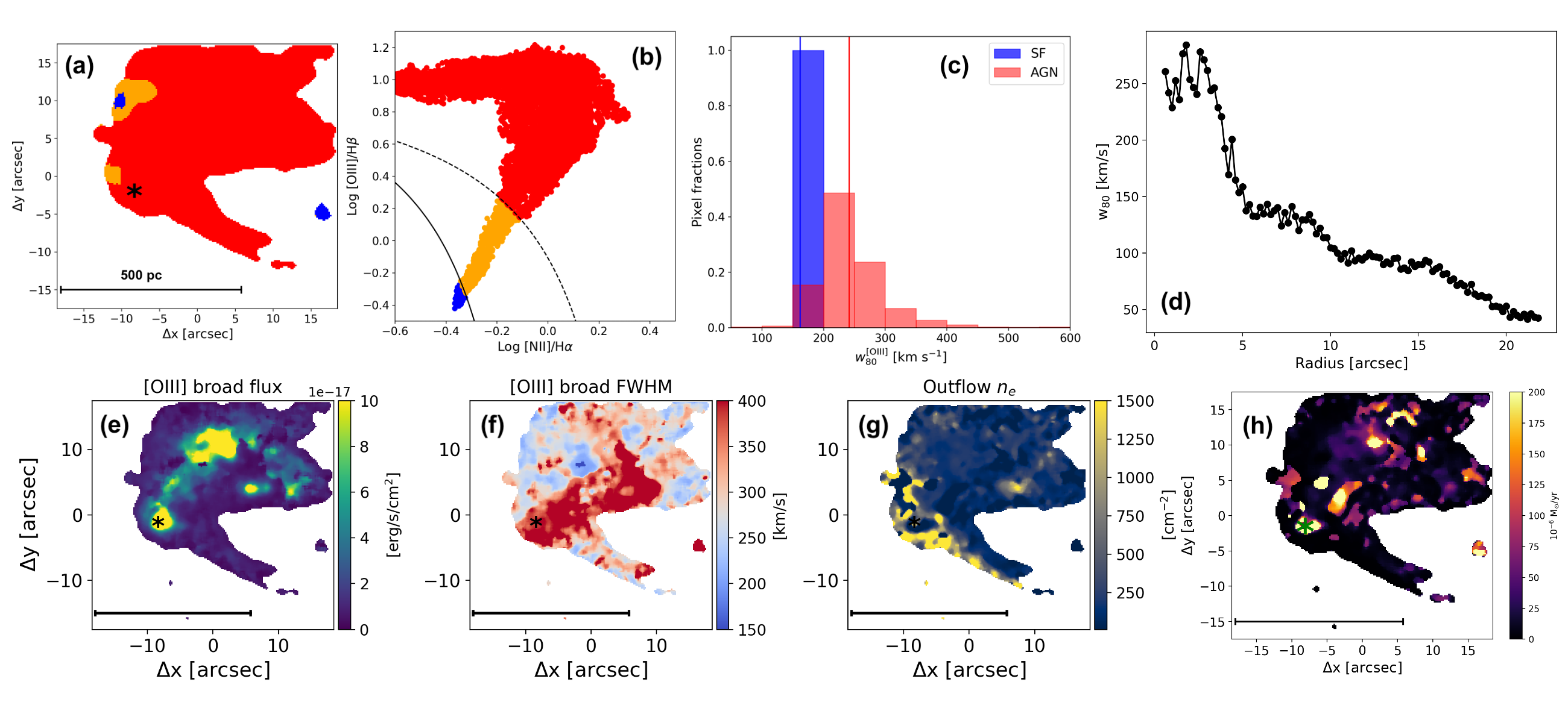
The possible presence of linear correlation between the parameter from the integrated spectrum and suggests a possible role of the AGN in regulating the kinematics of the ionised gas. We therefore investigated whether the evidence of such an AGN impact on the [O iii] based ionised gas velocity is also present in the resolved data. Therefore, we first made use of the BPT diagnostic maps (Baldwin et al. 1981; Veilleux & Osterbrock 1987, Baldwin, Phillips & Terlevich:) to identify pixels or regions ionised by the AGN, star formation or composite sources (Dopita et al. 2014; Belfiore et al. 2016; Davies et al. 2017; Kakkad et al. 2018, e.g.,). This is shown in the top panels of Fig. 7. We then compare the [O iii] distribution (after correcting for the spectral resolution) in the pixels ionised by AGN and star formation, as shown in the bottom right panel of Fig. 7. The BPT maps and distribution plots for the rest of the AGN sample presented in this paper are moved to the Appendix A.
Figure 7 clearly shows that the pixels or regions ionised by the AGN are skewed towards higher [O iii] values in NGC 7469. Star forming regions show a mean value of 240150 km s-1, while the AGN ionised regions show a higher fraction of values greater than 600 km s-1, with a mean of 360140 km s-1. Similar distributions have previously been observed in the case of MaNGA galaxies in Wylezalek et al. 2020 where the AGN ionised pixels show a much higher velocity compared to star formation ionised pixels. The bottom right panel in Fig. 7 shows that even with the finer sampling of higher spatially resolved MUSE data (compared with the lower resolution and coarsely sampled MaNGA sample), the previous literature results hold true. We note that this does not mean that the spaxels with AGN ionisation will necessarily show higher [O iii] value, as from figure 7 it is clear that even spaxels with AGN ionisation can show lower values. However, the AGN ionised regions will tend to show a collectively higher ionised gas velocity dispersion than the star forming pixels. In most of the cases, regions close to the AGN (which are clearly in the AGN ionisation region of the BPT diagram) show higher values. The results in Fig. 7 are therefore indicative of AGN activity having a greater impact on the kinematics of the ionised gas compared to star formation processes. The radial profiles (shown in the Appendix for individual galaxies) show a common trend that the values uniformly drop from the centre. However this is not always true as apparent from the distribution in NGC 7469 in Figs. 7 (bottom left panel) & 38 (panel d) and NGC 1365 in Fig. 23. The value increases from the AGN location, peaking at a distance of a few arcsec before dropping off at larger distances.
So far in this section we focused on the overall [O iii] line profile to indicate that the AGN has an impact on the width () of the [O iii] line. However, as mentioned earlier, we make use of the narrow and broad Gaussian decomposition to define a systemic gas (non-outflowing component) and the outflowing component respectively. Figure 8 shows an example of the narrow and broad Gaussian width distributions in NGC 7469, which supports this assumption for the analysis presented in this paper. The top left panel of Fig. 8 shows the centroid distribution of the narrow Gaussian component which shows a smooth rotation-like profile about an axis oriented approximately along the S-W direction. Such a smooth profile is not present in the centroid map of the broad component (top right panel in Fig. 8). Furthermore, the bottom panel in Fig. 8 shows the width (FWHM) distribution of the individual narrow and broad Gaussian components across the MUSE FoV. The narrow component width is always less than 250 km s-1, while the broad component reaches values of >600 km s-1 in some pixels, suggesting that this component is indeed tracing the high velocity outflowing gas possibly driven by the AGN (Luminari et al. 2021, e.g.,).
5.2 Resolved mass outflow rate maps
In this and the next sections, we show the resolved ionised gas mass outflow rate maps derived from spaxel-by-spaxel analysis and compare these values with measurements from the integrated fibre or slit spectra.

Figure 9 shows the outflow flux (left panel), velocity (FWHM, middle panel) and the electron density (right panel) distribution in NGC 7469, one of the galaxies in the BASS-MUSE sample as an example. These maps are obtained from the broad Gaussian component of the [O iii] line. Specifically in the case of NGC 7469, the outflow flux is concentrated close to the AGN location, marked by the black star, and the flux significantly drops with increasing distance from the AGN (by a factor of 10). Similar to the flux distribution, the outflow velocity defined by the width (FWHM) of the broad Gaussian, is also maximum at the center (1000 km s-1) and falls to 200 km s-1 towards the spiral arms. However, this drop is not uniform as the velocity and flux distributions both show clumpy profiles within the outflowing medium. We note that the outflow across the FoV might not be entirely due to the AGN, as the asymmetry in the [O iii] line profile could result from residual turbulence from star formation or supernovae driven winds (Davies et al. 2019; Avery et al. 2021; Herrera-Camus et al. 2021, e.g.,). The electron density map also shows a non-uniform distribution, similar to the ones observed previously in the literature with lower spatial resolution data (Kakkad et al. 2018, e.g.,).
Several galaxies in the BASS-MUSE sample also show a bi-conical ionisation morphology such as IC 1657, NGC 1365 (Venturi et al. 2018, e.g.,), NGC 2992 (Veilleux et al. 2001, e.g.,) and Mrk 463 (Treister et al. 2018). Often the outflow flux is concentrated towards the tip of this ionisation cone and falls off as a function of distance from the AGN. The outflow velocity and density, on the other hand, are distributed in the form of clumps within this ionisation cone. This is expected as the gas might interact with the stars and the dust within the ISM leading to non-uniform distribution of these quantities. The flux, velocity and electron density maps for the rest of the sample are shown in the Appendix A.

The outflow luminosity does not represent the distribution of the ionised gas mass or the mass outflow rate. This is because the outflow mass and the mass outflow rates are dependent on the three quantities – flux, velocity and electron density – as apparent from Eqs. 1 and 3. The ionised gas mass outflow rate map of NGC 7469 is shown in Fig. 10. The mass outflow rate distribution is non-uniform across the FoV and is concentrated along an arc towards the SE direction. The arc-like distribution in the mass outflow rate is also observed in several other galaxies such as NGC 5995 and 3C403. Such outflow morphology could be indicative of expansion of the ionised gas in the form of spherical shells from the AGN location. Within the spiral arms, such as in the case of NGC 7469, the outflow mass is negligible compared to regions close to the AGN, suggesting that the regions close to the AGN dominate the outflow mass as well as the outflow rate budget. We further discuss the outflow rates close to the AGN location later in this section.
The total instantaneous outflow rates () derived from the resolved maps are in the range 0.2–275 M⊙ yr-1, which are nearly consistent with previously published values in the literature for some of the galaxies presented in this paper (Venturi et al. 2018; Treister et al. 2018, e.g., NGC 1365 and Mrk 463, ). Table 2 also reports the mass outflow rate within the central 3″ of these outflow rate maps, outflow rate obtained from fibre () or slit () spectra and the outflow rate if the electron density is assumed to be 200 cm-3 (), a commonly adopted value in the literature (Fiore et al. 2017; Davies et al. 2020a, e.g.,).
Table 2 highlights that the outflow rate values are highly dependent on the method of spectral extraction. The ratio between and the time-averaged mass outflow rate obtained from fibre or slit spectra ( or ) ranges from 0.4–525 with a mean of 100. In other words, is on average about two orders of magnitude higher than or . To understand the difference between the two methods, we also compared the outflow mass obtained using the pixel-by-pixel analysis and using the fibre and slit aperture integrated spectra. The ratio of the outflow masses obtained from the resolved data to that of fibre or slit aperture spectra is in the range 0.01–130, with a mean ratio of 20 i.e. summed local outflow masses are an order of magnitude higher than outflow masses calculated from integrated spectra. Therefore, the observed difference in the mass outflow rate values could be a consequence of the fact that in the resolved maps, the outflow mass is calculated from a larger area (entire galaxy) compared to integrated spectra where the mass is obtained from a limited aperture size. Furthermore, these differences are also expected due to the different equations used in the computation of mass outflow rates, as described in Sect. 4.2. The summed instantaneous outflow rates are higher than the time-averaged integrated measurements by a factor of R/R.
A further important insight is obtained by calculating the mass outflow rate from a 3″ aperture on the resolved maps, (so as to match the area with the fibre extraction spectrum). We find that the mean ratio of to is 35. The average fraction of mass outflow rate concentrated in a 3″ region centred on the AGN (i.e. /) is 55% i.e. roughly half of the total instantaneous outflow rate is concentrated in the central 3″.
We do not make a distinction in the source of ionisation while calculating the mass outflow rates. Therefore, the entire FoV is used to calculate the local instantaneous mass outflow rates. This is also to ensure that all the outflowing gas is taken into account while calculating the mass outflow rates. As one of the main aims of this paper is to compare the local instantaneous mass outflow rate values (obtained from resolved maps) with that of the time averaged values (obtained from the integrated spectra) and that the scaling relations with the time-averaged values are not distinguished based on the source of ionisation, we do not make the distinction for consistency between the two measurements. Also, 90% of the mass outflow rate comes from AGN-ionised regions and 16 out of the 22 galaxies presented in the paper have their field-of-view dominated by AGN ionisation. Therefore, our results would not change significantly if only AGN ionised regions are used.
We also analyse the values of electron density derived from the outflowing component of [S ii] doublet for integrated fibre and slit spectra. We use Eq. 2 to derive the electron density from the outflowing components of the [S ii] doublet emission lines. Figure 11 shows the distribution of the outflow electron density obtained from the integrated spectra, which is in the range 10–1800 cm-3. We find a median electron density value of 300 cm-3, which is similar to the commonly assumed density value of 200 cm-3 in the literature (Fiore et al. 2017, e.g.,). This density is much lower than other integrated spectra studies targeting low redshift X-ray AGN hosts (Perna et al. 2017, e.g.,). However, there is a large range in the calculated densities, which depend on the method of spectral extraction and the slit orientation.
To summarise, the summed instantaneous mass outflow rates from resolved data show a higher outflow rate value than time-averaged outflow rates from integrated spectra. This is due to a combination of the equations used in the computation of these quantities and that a larger mass is incorporated with the larger FoV in the instantaneous case. The resolved outflow rate maps provide a means to incorporate variable outflow density, velocity and flux distribution to give a realistic picture of the distribution of the outflow mass across the host galaxies.


| BASS ID | Target | Log | Log | Log | Log | Log | |||
| km s-1 | km s-1 | M⊙/yr | M⊙/yr | M⊙/yr | M⊙/yr | M⊙/yr | % | ||
| (1) | (2) | (3) | (4) | (5) | (6) | (7) | (8) | (9) | (10) |
| 57 | 3C033 | 565 | 495 | -0.76 | -1.26 | -0.59 | -0.91 | -0.54 | 32 |
| 58 | NGC 424 | 814 | 740 | 1.42 | 1.40 | -1.00 | -1.30 | -0.25 | 95 |
| 62 | IC 1657 | 370 | 370 | -0.01 | -1.28 | -2.08 | -2.19 | -2.24 | 5 |
| 127 | HE 0224-2834 | 495 | 495 | 0.62 | 0.44 | -0.95 | -1.06 | -0.91 | 66 |
| 134 | NGC 985 | 574 | 574 | 1.67 | 1.63 | 1.10 | 1.02 | -0.20 | 91 |
| 184 | NGC 1365 | 298 | 298 | 0.14 | -2.50 | -2.28 | -2.34 | -2.05 | <1 |
| 197 | HE 0351+0240 | 289 | 289 | 0.01 | -0.18 | -1.68 | -0.79 | -1.55 | 64 |
| 213 | HE 0412-0803 | 361 | 361 | 1.29 | 1.14 | -0.37 | -0.45 | -0.04 | 70 |
| 216 | NGC 1566 | 522 | 522 | -0.22 | -0.69 | -2.18 | -0.15 | -1.43 | 33 |
| 471 | NGC 2992 | 595 | 595 | 0.52 | -1.06 | -1.69 | -1.79 | -1.08 | 3 |
| 501 | HE1029-1401 | 1449 | 1449 | 1.55 | 1.53 | 1.58 | 0.04 | 0.28 | 95 |
| 653 | NGC 4941 | 448 | 448 | -0.55 | -1.11 | -1.96 | -2.04 | -1.27 | 28 |
| 703 | Mrk 463 | 1070 | 1141 | 2.44 | 2.37 | 0.33 | -0.25 | 0.68 | 85 |
| 711 | Circinus | 299 | 299 | -0.26 | -0.96 | -2.98 | -3.18 | -2.30 | 20 |
| 731 | NGC 5643 | 448 | 522 | 0.35 | 0.09 | -1.72 | -1.83 | -1.08 | 55 |
| 783 | NGC 5995 | 804 | 804 | 0.13 | -0.53 | -1.59 | -1.69 | -1.62 | 20 |
| 817 | 2MASX J1631+2352 | 778 | 778 | 0.60 | 0.55 | 0.26 | 0.20 | -1.04 | 89 |
| 1051 | 3C403 | 566 | 566 | 0.24 | -0.05 | -1.90 | -0.96 | -1.96 | 51 |
| 1092 | IC 5063 | 518 | 444 | 1.25 | 0.96 | 0.54 | -0.46 | -0.76 | 51 |
| 1151 | 3C445 | 638 | 638 | 2.03 | 1.99 | 1.32 | 1.19 | 0.02 | 91 |
| 1182 | NGC 7469 | 663 | 663 | 0.67 | 0.51 | -0.83 | 1.02 | -0.23 | 70 |
| 1183 | Mrk 926 | 644 | 644 | 1.38 | 1.33 | -0.03 | -0.11 | 0.16 | 89 |
5.3 Mass outflow rate scaling relations
Several publications in the literature have investigated the presence or absence of correlations between the outflow properties and the AGN properties in the different ionised, molecular and neutral gas phases (Cicone et al. 2014; Cicone et al. 2018; Carniani et al. 2015; Fiore et al. 2017; Kakkad et al. 2020; Fluetsch et al. 2020; Rojas et al. 2020, e.g.,). Most of these are based on integrated spectra with fibre or slit spectroscopy or marginally resolved IFS data. Using the resolved MUSE data set, we investigate if the relations between outflow properties and the AGN properties change with the aperture or underlying methods of analysis.
Scaling relations between the [O iii] velocity dispersion () and , and were already presented in Sect. 5.1, where correlations (p-value0.05) were only suggestive in the case of . However, as we stressed previously, the mass outflow rate depends not only on velocity dispersion but also on the flux/luminosity and electron density. Thus, we revisit this theme, focusing on correlations between the mass outflow rates obtained from different methods and the AGN properties, namely , and . We compute the Pearson’s r correlation coefficient implementation within pymccorrelation package (Curran 2014; Privon et al. 2020, seee).
Figure 12 shows the relations of the summed instantaneous mass outflow rates obtained from the resolved mass outflow rate map (, solid red circles), and time-averaged outflow rates from the integrated fibre spectra (, open blue circles) and slit spectra (, solid blue squares) versus (left panel), (middle panel) and (right panel), respectively. The results from the Pearson correlation tests between mass outflow rates derived from the different methods and the AGN properties are reported in Table 3.
versus : Similar to the case of the velocity dispersion, the mass outflow rates show a maximum probability of correlation with the bolometric luminosity. The null hypothesis for a non-correlation (p-value) with is 1% for all methods of outflow rates computations (although considering uncertainties, the correlation between and is relatively weak). The correlation with is strongest in the case of time-averaged mass outflow rates obtained from the fibre spectra. The outflow rates derived from summed resolved data have a higher intercept and flatter slope compared to the integrated spectra obtained from fibre or slit aperture (0.510.03 in the former case compared to 1.040.05 & 0.790.05 in the latter). The p-value for the outflow rate derived from slit spectra versus is slightly higher at 0.003, compared to 2.0e-4 in the case of fibre spectra. We note here that in the case of the slit spectroscopy, the mass outflow rate values depend on the slit orientation. Different slit orientations were explored and Table 2 reports the values for slit spectroscopy which show the most extreme differences with respect to the circular aperture. However, despite these differences, the time-averaged mass outflow rates obtained from fibre and slit spectra roughly cover the same parameter space in Fig. 12. We also note that the p-value reduces in the case of outflow rate values extracted from the central 3″aperture in the resolved maps (), compared to the total summed resolved map (). This result might already suggest that the AGN influence on the ISM is the strongest within the inner one kiloparsec of host galaxies.
versus and : The mass outflow rates show a weaker correlations (or no correlation) with the black hole mass and Eddington ratio, compared to the bolometric luminosity. However, we find a strong correlation between the time-averaged outflow rate value from fibre spectra versus with a p-value of 0.01, again highlighting that the presence or absence of correlation is highly dependent on the observation and analysis method. These correlations will be further discussed in the context of the driving mechanism of outflows in Sect. 6.
We note that there is no significant change in the presence or absence of correlations if we assume a constant density value in the case of time-averaged mass outflow rate values, although the relative slopes might be different. This is apparent from the relations in Table 3. We also compare these correlations with the results previously published in the literature for ionised and molecular gas outflows, as shown in Fig. 13 (Cicone et al. 2014; Cicone et al. 2018; Walter et al. 2017; Zschaechner et al. 2018b, e.g.,). For simplicity, we only consider the relations with the bolometric luminosity. The ionised gas outflows are shown in red, blue, yellow and magenta curves/shaded regions, while the molecular outflow scaling relation is shown as green curve. The shaded regions correspond to an assumed electron density range of 200–5000 cm-3 in ionised outflows. The mass outflow rate scaling relation from the fibre integrated spectra of the BASS-MUSE sample is consistent with the literature results, which are also obtained from integrated spectroscopy using fibre or slit. The summed instantaneous outflow rates obtained from resolved data are clearly 1–2 orders of magnitude higher than the time-averaged outflow rate values from the integrated spectra from the literature. The difference is more pronounced at lower bolometric luminosities. The molecular outflows still seem to dominate the outflowing gas content in low as well as high redshift galaxies and across a wide range of bolometric luminosities. However, similar analysis as the one presented in this paper, will be required to investigate the scaling relations and observational biases in the case of molecular outflows (Treister et al. 2018; Perna et al. 2021, e.g., MODA, PUMA surveys). This will require high spatial resolution and deeper observations with sub-mm facilities such as ALMA, VLA, PdBI and SMA (Sun et al. 2014; Brusa et al. 2018, see also).
| Relation | Correlation | p-value | Slope |
|---|---|---|---|
| coefficient | |||
| Relations with | |||
| vs. Lbol | 0.52 | 0.02 | 0.1020.001 |
| vs. Lbol | 0.50 | 0.02 | 0.0960.002 |
| vs. | 0.58 | 0.003 | 0.1280.002 |
| vs. | 0.58 | 0.004 | 0.1260.002 |
| vs. Lbol | 0.54 | 0.01 | 0.510.03 |
| vs. Lbol | 0.63 | 0.01 | 0.910.06 |
| vs. Lbol | 0.73 | 0.01 | 1.040.05 |
| vs. Lbol | 0.62 | 0.01 | 0.790.05 |
| vs. Lbol | 0.58 | 0.004 | 0.560.03 |
| Relations with | |||
| vs. MBH | 0.37 | 0.10 | – |
| vs. MBH | 0.32 | 0.15 | – |
| vs. | 0.36 | 0.11 | – |
| vs. | 0.34 | 0.12 | – |
| vs. MBH | 0.18 | 0.34 | – |
| vs. MBH | 0.29 | 0.18 | – |
| vs. MBH | 0.56 | 0.009 | 0.750.08 |
| vs. MBH | 0.34 | 0.13 | – |
| vs. MBH | 0.33 | 0.13 | – |
| Relations with | |||
| vs. | 0.00 | 0.22 | – |
| vs. | 0.03 | 0.21 | – |
| vs. | 0.08 | 0.42 | – |
| vs. | 0.08 | 0.40 | – |
| vs. | 0.33 | 0.14 | – |
| vs. | 0.27 | 0.17 | – |
| vs. | 0.13 | 0.46 | – |
| vs. | 0.20 | 0.35 | – |
| vs. | 0.25 | 0.24 | – |
| Relations with | |||
| vs. | 0.17 | 0.47 | – |
| vs. | 0.14 | 0.53 | – |
| vs. | 0.47 | 0.12 | |
| vs. | 0.33 | 0.27 | |
| vs. | 0.13 | 0.39 | – |
| vs. | 0.25 | 0.37 | – |
| vs. | 0.42 | 0.17 | – |
| vs. | 0.43 | 0.16 | – |
| vs. | 0.23 | 0.39 | – |
6 Discussion
In this paper, we have presented the impact of observational bias and the methods of analysis on the observed correlations between the properties of ionised gas outflows and the AGN. We showed that the parameters of the linear correlations change depending on whether the individual data points are obtained from a spatially resolved or integrated fibre/slit spectroscopy or from assumed values while modelling the outflows. In this section, we discuss the implications of the results presented in Sect. 5 and explore the possible reasons for the presence or absence of correlations. By comparing the scaling relations obtained from the resolved data and the literature (or integrated fibre/slit spectra), we will also provide a means to correct (or cross-calibrate) for observational biases in future studies. Lastly, we will discuss the nature of these outflows in the context of predictions from current state-of-the-art hydrodynamical simulations.
For 80% of the galaxies, the [O iii] parameter (a measure of ionised gas kinematics) derived from the integrated fibre or slit spectra show consistent values, suggesting a minor dependence of the parameter on observational method. The values correlate with the AGN bolometric luminosity, but not the black hole mass or Eddington ratio. Also, in the resolved data, the distribution is skewed towards larger values in regions ionised by the AGN compared to the star formation ionised regions. These results, therefore, suggest that the ionised gas kinematics is dependent on the power of the ionising radiation from the central source. However, the line broadening could also result from shocks (Rich et al. 2014, e.g.,) induced in targets that are undergoing or recently underwent a merger (Treister et al. 2018, e.g., Mrk 463). However, since the fraction of mergers in our sample is relatively low, the AGN radiation seems to be the dominant mechanism behind the observed turbulence. We note that unlike observations at high redshift, where high velocity (800 km s-1) ionised gas is observed in a few kiloparsec scales, the low redshift X-ray AGN show high velocity gas restricted to sub-kiloparsec scales.
The mass outflow rate maps show the distribution of instantaneous outflow rates through local ionised clouds. Although we observe a diverse morphology in the outflow rate maps themselves, some targets such as NGC 7469 (Fig. 10) notably show a semi-arc like structure which may suggest a spherical propagation of the outflow closer to the AGN location. Several numerical simulations invoke or predict a spherical or semi-spherical shockfront that results from an AGN outburst (Gabor & Bournaud 2014; Nayakshin 2014; Zubovas & Nayakshin 2014, e.g.,). A thin shell-like outflow morphology was also proposed in Husemann et al. 2019 for a nearby AGN, HE 1353-1917. The observed mass outflow rate maps are also consistent with recent results from resolved spectroscopy in the literature (Revalski et al. 2021, e.g.,) where the mass outflow rate is shown to have a peak value at a distance of 500–1500 pc from the AGN location, before dropping off at larger distances.

A comparison of the resolved mass outflow rate maps and the mass outflow rate calculated from fibre or slit spectra show that the values and their scaling relations with AGN properties can highly depend on the analysis method, as apparent from Fig. 12 and Tables 2 and 3. The mass outflow rates show a correlation with the AGN bolometric luminosity, regardless of the calculations using integrated or spatially resolved data. The fact that we observe the correlations with the bolometric luminosity suggests that the AGN radiation may be, at least in part, responsible for driving these outflows. The probability of correlation increases (lower p-value in Table 3) if the mass outflow rates are obtained from time-averaged values of the integrated fibre or slit spectra. Between the outflow rates obtained from the fibre and slit spectra, the correlations are stronger in the case of fibre spectra. This further indicates possible AGN driven nature of the ionised gas outflows over the lifetime of the outflow (R/). And finally, in the case of instantaneous mass outflow rates from resolved maps, the correlation is stronger when the mass outflow rate values extracted from the central 3″aperture is considered, compared to the summed outflow rate integrated over the entire FoV. Therefore, the AGN radiation shows the strongest influence on the ionised gas in its vicinity compared to the gas in the galactic outskirts. This is also supported by the fact that we do not observe high velocity winds in the galaxy outskirts, unless the system is disturbed due to external factors such as mergers.
As described in Sect. 5, the observed difference in the summed instantaneous mass outflow rate from the resolved maps and the time-averaged outflow rate from the integrated spectra could be due to a combination of higher outflow mass from the larger FoV of the resolved maps and the radius factor in the respective equations. One may use Fig. 12 to define an “effective electron density” for summed instantaneous outflows, . The effective electron density is the density value that can be used in the time-averaged outflow rate equation to derive the summed instantaneous outflow rate i.e. this value can be used to cross-calibrate between the instantaneous and time-averaged methods. We find that the has a value of 10 cm-3. Therefore, if the mass outflow rate calculations need to be made from integrated spectra using the biconical outflow model with uniform density of ionised gas, an electron density of 10 cm-3 would provide outflow rate values consistent with those of resolved maps presented in this paper.
The correlation of ionised gas mass outflow rates and the bolometric luminosity has been reported in several works (Fiore et al. 2017, e.g., see a literature compilation in). Recent spatially resolved observations with STIS/HST show that the mass outflow rates and the kinetic energy seem to monotonically increase with the AGN luminosity for 6 nearby AGN (Revalski et al. 2021). However, we note that contrary results have also been reported in the literature, where no correlation is observed between the outflow rates and the bolometric luminosity (Baron & Netzer 2019; Davies et al. 2020a, e.g.,) for a similar range of bolometric luminosity also explored in this paper. One of the main difference in these works is that the electron density is calculated based on the ionisation parameter, the AGN luminosity and the distance of the outflowing gas from the AGN location, also called method. The method is sensitive to higher density values compared to the [S ii] doublet method used in this paper and as a result, Baron & Netzer 2019 and Davies et al. 2020a find electron densities that are 3–100 times larger than the ones reported in this paper. Furthermore, the bolometric luminosity ranges compared in these works are slightly lower than the ones displayed by the sample in this paper (This paper, 3 dex –1045.5 erg s-1, Davies et al. 2020a: 2 dex 1043–1044.5 and Baron & Netzer 2019: 2 dex 1043.5–1045.5). Similarly, Rojas et al. 2020 use a constant density value of 104.5 cm-3 for their (time-averaged) mass outflow rate calculations for a sub-sample of BASS galaxies, based on integrated spectrum measurements. The observed differences in the outflow rate values in Rojas et al. 2020 and this paper can be attributed to these different methodologies. A robust comparison between these works, therefore, cannot be made within the scope of this paper and a future work will address the spatially resolved mass outflow rates considering electron density determination using the multiple methods. However, upon using the assumed electron densities in these works (which are based on the electron density derived from the [S ii] doublet values), the scatter in the is reduced, which suggests that the scaling relations are indeed subject to the methods of analysis. We estimate a maximum error in the mass outflow rate of 0.5 dex and in the bolometric luminosity of 0.3 dex. The presence of correlation in this work will also be observed after taking into account the errors in the different quantities.
We find a weak or no correlation of any of the outflow quantities, namely the outflow velocity and mass outflow rate, with the black hole mass and the Eddington ratio. Therefore, the observed outflows for the sample used in this paper cannot be explained by radiation pressure driven winds from the accretion disk. Extra-galactic studies in the literature have also shed light on the impact of radio jets in driving outflows in multiple gas phases, via jet-mode feedback (Villar Martín et al. 2014; Nesvadba et al. 2017; Santoro et al. 2018; Molyneux et al. 2019; Jarvis et al. 2021, also called radio-mode or mechanical-mode of feedback, e.g.,). Several theoretical simulations support a scenario where radio jets transfer the energy into the ISM, which can also create a clumpy distribution of gas (Sutherland & Bicknell 2007; Wagner et al. 2012; Cielo et al. 2018; Mukherjee et al. 2018b, e.g.,). Therefore, we also explore the presence of any correlation of the outflow properties with the radio luminosity in Fig. 14. We obtain the 1.4 GHz radio fluxes from Véron-Cetty & Véron 2010 catalogue, which are available for 12 out of the 22 AGN presented in this paper. The radio luminosity, , of our targets is in the range 1021–1026 W/Hz (5 dex) and Table 3 reports the correlation test results of various outflow properties presented earlier, but with the radio luminosity. Similar to the Eddington ratio, we do not find a robust correlation with the radio luminosity.
The presence of non-correlations of total mass outflow rate from resolved maps with both the Eddington ratio and the radio luminosity can be an interpretation of the fact that the observed outflows may be a combination of radiation pressure driven or thermal winds, radio jets and external influences such as shocks induced by mergers. Therefore, correlations with a single quantity may not exist. Relatively weaker processes such as star formation could also contribute to the scatter in the scaling relations (DiPompeo et al. 2018, e.g.,). This is evident from an in-depth analysis of individual targets that have been published in the literature. For instance, ionised and molecular gas observations of IC 5063 have shown evidence of jet-ISM interaction in this system (Kulkarni et al. 1998; Morganti et al. 2015; Tadhunter et al. 2014; Dasyra et al. 2015; Oosterloo et al. 2017; Mukherjee et al. 2018a; Venturi et al. 2021, e.g.,). Jet-ISM interaction has also been proposed in some of the 3C sources, part of the MURALES survey (Balmaverde et al. 2019; Balmaverde et al. 2021, e.g.,). Similarly, Mrk 463 is a late-stage merger and the observed outflow could be due to the accretion disk triggered by the merging activity (Treister et al. 2018, see). Thermal winds are believed to be driving the outflows in NGC 2992 in the biconical morphology, also observed in the MUSE data presented in this paper (Veilleux et al. 2001, e.g.,), while in the low luminosity AGN in NGC 1365, star formation is also inferred to be driving the outflows (Venturi et al. 2018, e.g.,). In summary, all these processes contribute to the observed mass outflow rate scaling relations with the bolometric luminosity. At redshift corresponding to cosmic noon (z2–3), the black hole accretion activity is expected to be at its maximum (Silk & Mamon 2012; Madau & Dickinson 2014, e.g.,). Therefore, the chances are that the high redshift surveys pick up a large fraction of targets where accretion disk driven winds are dominant, which might explain the observed scaling relations with the Eddington ratio at this epoch (Kakkad et al. 2020, e.g.,).
We also note that other emission lines such as H and H have also been used in the literature to derive the properties of ionised gas outflows. The H line is usually faint in the NLR and the H is more susceptible to dust extinction effects compared to the [O iii] line. Furthermore, H could also be contaminated by the closely spaced [N ii]6549, 6585 lines due to blending in the case of high velocity outflows. These factors may partly explain the observed differences between the results presented in this paper and in Ruschel-Dutra et al. 2021 who also report the ionised outflow properties of 30 low redshift AGN host galaxies using the H line. For example, Ruschel-Dutra et al. 2021 find mass outflow rates in the range Log = -3.91–2.38 with a median value of -2.1, while the local instantaneous mass outflow rates presented in this paper are in the range Log = -0.76–2.44, with a median value of 0.56, nearly two orders of magnitude more than that in Ruschel-Dutra et al. 2021. Furthermore, only two sources in Ruschel-Dutra et al. 2021 show a coupling efficiency 1%, in contrast to the methods used in this paper where some sources show much higher coupling efficiencies (discussed below). The dependence of outflow properties on different diagnostic lines will be explored in a future work.
Lastly, we calculate the fraction of AGN bolometric luminosity that is coupled to the ISM via kinetic energy of the observed ionised outflows, = 1/2. Cosmological simulations invoking AGN feedback are able to reproduce observed AGN host galaxy correlations, such as the ones presented in this paper, by requiring that 5-10% of the energy from the AGN is coupled with the ISM of the host galaxy (Fabian 1999; Springel et al. 2005; Kurosawa et al. 2009, e.g.,). Observationally, determination of this coupling efficiency has been challenging due to the large systematic uncertainties in the derivation of this quantity, which we attempt to resolve using the IFS data presented in this paper. We derive and values from the resolved maps resulting in a resolved kinetic energy map. Figure 15 shows the total kinetic energy obtained from the resolved map versus . The different linear curves correspond to the coupling factors of 0.1%, 1%, 10% and 100%. We find a wide range in the coupling efficiency with ionised gas outflows from 0.1% to 40% (median 1%), which seems to monotonically increase with the bolometric luminosity of the AGN. This is similar to trends previously found in the literature, although with more scatter (Carniani et al. 2015, e.g.,). The kinetic energy values reported in this paper are higher than the ones reported in the analysis of BASS sub-sample in Rojas et al. 2020, which could be a combination of the fact that integrated spectra was used in Rojas et al. 2020, resulting in time-averaged outflow properties, and that a much higher electron density value of 104.5 cm-3 was used (both of which would approximately compensate for the observed differences between the two papers).
Calculation of the AGN luminosity coupling with outflow kinetic energy is further complicated with the fact that the outflows may not be in single gas phase, but may consist of ionised, molecular and neutral gas components (Rupke & Veilleux 2013; Feruglio et al. 2015; Cicone et al. 2018; Husemann et al. 2019; Baron et al. 2020; Fluetsch et al. 2020; Herrera-Camus et al. 2020; Perna et al. 2020; Treister et al. 2020, e.g.,). Similar mass outflow rate maps with different gas phases need to be traced to get a true picture of the extent of AGN influence on the ISM. While this paper characterises the properties of spatially resolved outflows, the impact that these outflows have on the host galaxy properties such as the overall molecular gas content and star formation rate will be addressed in future publications.

7 Summary and Conclusions
In this paper, we presented the [O iii]5007 based ionised gas outflow properties, specifically the outflow velocity, mass outflow rates and kinetic energy, in 22 low redshift X-ray AGN host galaxies selected from the BASS survey. We have used optical IFS capabilities of MUSE instrument on board the VLT to understand how observational and analysis methods can influence these outflow properties and their correlations with the AGN properties, namely , , and . Specifically, we used a 3″ circular aperture and a rectangular aperture, to mimic the fibre and slit observations that are frequently used in the literature. We modelled the emission lines using multi-Gaussian functions and the broad Gaussian function was used as a proxy for the outflowing component. From the spectra extracted from these apertures, we computed the [O iii] velocity dispersion and time-averaged outflow rates and kinetic energies over the lifetime of the outflows. The electron density of the outflows are determined using the outflowing component of [S ii]6716, 6731 emission lines. We also derived instantaneous mass outflow rate in every pixel for all the galaxies, which incorporates variable outflow flux, density and velocity within the outflowing media. Finally, we investigated the presence of scaling relations between these outflow properties from multiple methods versus the AGN properties. The scaling relations are explored for the following range in the AGN properties: – erg s-1; – M⊙; 0.002–1.062 and – W Hz-1. We enumerate here the main results from the analysis presented in this paper:
- 1.
Nearly 80% of the targets show consistent [O iii] values in the integrated spectra, irregardless of whether they are obtained from fibre or slit spectra. The differences in the 20% of the galaxies result from whether the slit orientation is aligned with the outflow. The [O iii] parameter shows a linear correlation with and a weak or no correlation with , and . The results of the scaling relations do not depend on whether the spectra is obtained from the fibre or slit aperture.
- 2.
A comparison between the maps and the BPT maps in each galaxy shows that the [O iii] values have higher values (120 km s-1) on average in AGN ionised regions compared to regions ionised purely by star formation, suggesting an AGN impact on the ionised gas kinematics. Furthermore, the narrow Gaussian component reproduces the rotation profiles of the host galaxies and the kinematic maps show that the FWHM of the narrow component is 250 km s-1 in most cases. The broad Gaussian map, on the other hand, shows a much wider distribution in its width (FWHM) with values reaching >600 km s-1 and therefore, treated as tracing the outflowing component.
- 3.
The summed local instantaneous mass outflow rate, obtained from the resolved maps is, on average, 2 orders of magnitude higher than the time-averaged mass outflow rate obtained from the integrated fibre or slit spectra. This difference is a due to a combination of higher outflow masses obtained via the larger area in the resolved maps and the respective equations used in the outflow rate computations of instantaneous and time-averaged values. The summed instantaneous mass outflow rates from the resolved maps is in the range 0.2–275 M⊙ yr-1, while the time-averaged outflow rate from the fibre aperture is in the range 0.001–38 M⊙ yr-1 and slit aperture 0.001–15 M⊙ yr-1. The time-averaged outflow rates are consistent with the values found in the literature using fibre or slit spectra.
- 4.
Both the instantaneous and the time-averaged mass outflow rates from fibre and slit apertures show a linear correlation with (p-value for non-correlation 0.01). The correlations are strongest (smaller p-value) with time-averaged outflow rate values obtained from the fibre aperture. In the case of instantaneous outflow rates from resolved maps, smaller p-values are obtained for correlations with when the outflow rates are summed over the central 3″ region, compared to the outflow rates summed over the entire FoV. These results suggest an efficient coupling between the AGN radiation and the ISM closer to the AGN location. We do find a weak or no correlation between the outflow rates obtained with the different methods and , or . This suggests that no single mechanism is dominant for driving the outflows in the low redshift sample presented in this paper.
- 5.
Lastly, we find the median outflow coupling, i.e. the ratio between the outflow kinetic energy and the bolometric luminosity to be 1%, although the entire range of coupling efficiency is between 0.1 and 40%.
Although this paper presents the outflow properties in a single gas phase i.e. the ionised gas, many of these galaxies are known to have outflows existing in other gas phases such as the molecular gas phase, which may have a larger energy budget compared to the ionised gas. Therefore future work will present outflows from other gas phases using current and upcoming instruments/facilities such as ALMA, JVLA, PdBI, NIRSpec/JWST, MIRI/JWST and ERIS/VLT. Furthermore, the high velocity outflows with [O iii] width >600 km s-1 are found closest to the AGN and are at times not resolved with the currently available MUSE data. Therefore, a future targeted follow-up at high resolution using AO instruments such as the Narrow Field Mode of MUSE would be key in characterising the outflow properties close to the AGN. Instruments on board the Extremely Large Telescope such as HARMONI (Thatte et al. 2010, e.g.,) will also play a key role in pushing such studies to even higher redshifts (where AGN with higher bolometric luminosity are detected) with increased sensitivity and spatial resolution.
Acknowledgements
We thank the referee for their useful suggestions. ET and FEB acknowledge support from ANID grants CATA-Basal AFB-170002 and FB210003 and FONDECYT Regular grant 1190818. ET acknowledges support from ANID Anillo ACT172033 and Millennium Nucleus NCN19_058 (TITANs). FEB acknowledges support from FONDECYT regular grant 1200495, Millennium Science Initiative ICN12_009. ARL acknowledges aupport from FONDECYT Postdoctorado project No. 3210157. MK acknowledges support from NASA through ADAP award NNH16CT03C. KO acknowledges support from the National Research Foundation of Korea (NRF-2020R1C1C1005462). CR acknowledges support from the Fondecyt Iniciacion grant 11190831 and ANID BASAL project FB210003. BT acknowledges support from the Israel Science Foundation (grant number 1849/19) and from the European Research Council (ERC) under the European Union’s Horizon 2020 research and innovation program (grant agreement number 950533). DK, ES, NDM and NG acknowledge the support from ESO for their studentship programme and Science Support Discretionary Funds. NDM and NG are grateful for the hospitality by ESO-Chile. FR acknowledges support from PRIN MIUR 2017 project “Black Hole winds and the Baryon Life Cycle of Galaxies: the stone-guest at the galaxy evolution supper”, contract 2017PH3WAT. RR thanks Conselho Nacional de Desenvolvimento Científico e Tecnológico ( CNPq, Proj. 311223/2020-6, 304927/2017-1 and 400352/2016-8), Fundação de amparo ’a pesquisa do Rio Grande do Sul (FAPERGS, Proj. 16/2551-0000251-7 and 19/1750-2), Coordenação de Aperfeiçoamento de Pessoal de Nível Superior (CAPES, Proj. 0001). Based on observations made with ESO telescopes at the La Silla Paranal Observatory under programmes 60.A-9100(K), 60.A-9339(A), 094.B-298, 094.B-0321, 094.B-0345, 095.B-0015, 095.B-0482, 095.B-0532, 095.B-0934, 096.D-0263, 096.B-0309, 097.B-0080, 097.D-0408, 099.B-0137, 0100.B-0116.
Data Availability
All the raw data analysed in this paper are publicly available in the ESO archive. The respective programme IDs from which these data are obtained are mentioned in the footnote in Sect. 2.
References
- Ahumada et al. (2020) Ahumada R., et al., 2020, ApJS, 249, 3
- Audibert et al. (2019) Audibert A., et al., 2019, A&A, 632, A33
- Avery et al. (2021) Avery C. R., et al., 2021, MNRAS, 503, 5134
- Bacon et al. (2010) Bacon R., et al., 2010, in Ground-based and Airborne Instrumentation for Astronomy III. p. 773508, doi:10.1117/12.856027
- Bacon et al. (2017) Bacon R., et al., 2017, A&A, 608, A1
- Bae & Woo (2016) Bae H.-J., Woo J.-H., 2016, ApJ, 828, 97
- Baldwin et al. (1981) Baldwin J. A., Phillips M. M., Terlevich R., 1981, PASP, 93, 5
- Balmaverde et al. (2019) Balmaverde B., et al., 2019, A&A, 632, A124
- Balmaverde et al. (2021) Balmaverde B., et al., 2021, A&A, 645, A12
- Baron & Netzer (2019) Baron D., Netzer H., 2019, MNRAS, 486, 4290
- Baron et al. (2020) Baron D., Netzer H., Davies R. I., Xavier Prochaska J., 2020, MNRAS, 494, 5396
- Barthelmy et al. (2005) Barthelmy S. D., et al., 2005, Space Sci. Rev., 120, 143
- Begelman et al. (2006) Begelman M. C., Volonteri M., Rees M. J., 2006, MNRAS, 370, 289
- Belfiore et al. (2016) Belfiore F., et al., 2016, MNRAS, 461, 3111
- Benson et al. (2003) Benson A. J., Bower R. G., Frenk C. S., Lacey C. G., Baugh C. M., Cole S., 2003, ApJ, 599, 38
- Bischetti et al. (2017) Bischetti M., et al., 2017, A&A, 598, A122
- Blanton et al. (2011) Blanton E. L., Randall S. W., Clarke T. E., Sarazin C. L., McNamara B. R., Douglass E. M., McDonald M., 2011, ApJ, 737, 99
- Brusa et al. (2016) Brusa M., et al., 2016, A&A, 588, A58
- Brusa et al. (2018) Brusa M., et al., 2018, A&A, 612, A29
- Bundy et al. (2015) Bundy K., et al., 2015, ApJ, 798, 7
- Cappellari (2017) Cappellari M., 2017, MNRAS, 466, 798
- Cappellari & Emsellem (2004) Cappellari M., Emsellem E., 2004, PASP, 116, 138
- Carniani et al. (2015) Carniani S., et al., 2015, A&A, 580, A102
- Carniani et al. (2016) Carniani S., et al., 2016, A&A, 591, A28
- Cicone et al. (2014) Cicone C., et al., 2014, A&A, 562, A21
- Cicone et al. (2018) Cicone C., Brusa M., Ramos Almeida C., Cresci G., Husemann B., Mainieri V., 2018, Nature Astronomy, 2, 176
- Cielo et al. (2018) Cielo S., Babul A., Antonuccio-Delogu V., Silk J., Volonteri M., 2018, A&A, 617, A58
- Costa et al. (2014) Costa T., Sijacki D., Haehnelt M. G., 2014, MNRAS, 444, 2355
- Crain et al. (2015) Crain R. A., et al., 2015, MNRAS, 450, 1937
- Cresci et al. (2017) Cresci G., Vanzi L., Telles E., Lanzuisi G., Brusa M., Mingozzi M., Sauvage M., Johnson K., 2017, A&A, 604, A101
- Curran (2014) Curran P. A., 2014, arXiv e-prints, p. arXiv:1411.3816
- Dasyra et al. (2015) Dasyra K. M., Bostrom A. C., Combes F., Vlahakis N., 2015, ApJ, 815, 34
- Davies et al. (2017) Davies R. L., et al., 2017, MNRAS, 470, 4974
- Davies et al. (2019) Davies R. L., et al., 2019, ApJ, 873, 122
- Davies et al. (2020a) Davies R., et al., 2020a, arXiv e-prints, p. arXiv:2003.06153
- Davies et al. (2020b) Davies R. L., et al., 2020b, ApJ, 894, 28
- Di Matteo et al. (2005) Di Matteo T., Springel V., Hernquist L., 2005, Nature, 433, 604
- DiPompeo et al. (2018) DiPompeo M. A., Hickox R. C., Carroll C. M., Runnoe J. C., Mullaney J. R., Fischer T. C., 2018, ApJ, 856, 76
- Dimitrijević et al. (2007) Dimitrijević M. S., Popović L. Č., Kovačević J., Dačić M., Ilić D., 2007, MNRAS, 374, 1181
- Diniz et al. (2019) Diniz M. R., Riffel R. A., Storchi-Bergmann T., Riffel R., 2019, MNRAS, 487, 3958
- Dopita et al. (2014) Dopita M. A., et al., 2014, A&A, 566, A41
- Dopita et al. (2015) Dopita M. A., et al., 2015, ApJS, 217, 12
- Durré & Mould (2018) Durré M., Mould J., 2018, ApJ, 867, 149
- Erroz-Ferrer et al. (2019) Erroz-Ferrer S., et al., 2019, MNRAS, 484, 5009
- Fabian (1999) Fabian A. C., 1999, MNRAS, 308, L39
- Fabian (2012) Fabian A. C., 2012, ARA&A, 50, 455
- Faucher-Giguère & Quataert (2012) Faucher-Giguère C.-A., Quataert E., 2012, MNRAS, 425, 605
- Feruglio et al. (2015) Feruglio C., et al., 2015, A&A, 583, A99
- Fiore et al. (2017) Fiore F., et al., 2017, A&A, 601, A143
- Fischer et al. (2013) Fischer T. C., Crenshaw D. M., Kraemer S. B., Schmitt H. R., 2013, ApJS, 209, 1
- Fluetsch et al. (2019) Fluetsch A., et al., 2019, MNRAS, 483, 4586
- Fluetsch et al. (2020) Fluetsch A., et al., 2020, arXiv e-prints, p. arXiv:2006.13232
- Gabor & Bournaud (2014) Gabor J. M., Bournaud F., 2014, MNRAS, 441, 1615
- García-Bernete et al. (2021) García-Bernete I., et al., 2021, A&A, 645, A21
- Gaspari et al. (2011) Gaspari M., Melioli C., Brighenti F., D’Ercole A., 2011, MNRAS, 411, 349
- Gehrels et al. (2004) Gehrels N., et al., 2004, ApJ, 611, 1005
- Genel et al. (2014) Genel S., et al., 2014, MNRAS, 445, 175
- Genzel et al. (2011) Genzel R., et al., 2011, ApJ, 733, 101
- Greene et al. (2011) Greene J. E., Zakamska N. L., Ho L. C., Barth A. J., 2011, ApJ, 732, 9
- Harrison et al. (2014) Harrison C. M., Alexander D. M., Mullaney J. R., Swinbank A. M., 2014, MNRAS, 441, 3306
- Harrison et al. (2018) Harrison C. M., Costa T., Tadhunter C. N., Flütsch A., Kakkad D., Perna M., Vietri G., 2018, Nature Astronomy, 2, 198
- Herrera-Camus et al. (2020) Herrera-Camus R., et al., 2020, A&A, 635, A47
- Herrera-Camus et al. (2021) Herrera-Camus R., et al., 2021, A&A, 649, A31
- Ho et al. (2016) Ho I. T., et al., 2016, Ap&SS, 361, 280
- Hopkins & Elvis (2010) Hopkins P. F., Elvis M., 2010, MNRAS, 401, 7
- Hopkins et al. (2016) Hopkins P. F., Torrey P., Faucher-Giguère C.-A., Quataert E., Murray N., 2016, MNRAS, 458, 816
- Husemann et al. (2019) Husemann B., et al., 2019, A&A, 627, A53
- Impellizzeri et al. (2019) Impellizzeri C. M. V., et al., 2019, ApJ, 884, L28
- Ishibashi & Fabian (2015) Ishibashi W., Fabian A. C., 2015, MNRAS, 451, 93
- Jarvis et al. (2021) Jarvis M. E., et al., 2021, MNRAS, 503, 1780
- Kaasinen et al. (2017) Kaasinen M., Bian F., Groves B., Kewley L. J., Gupta A., 2017, MNRAS, 465, 3220
- Kakkad et al. (2016) Kakkad D., et al., 2016, A&A, 592, A148
- Kakkad et al. (2018) Kakkad D., et al., 2018, A&A, 618, A6
- Kakkad et al. (2020) Kakkad D., et al., 2020, A&A, 642, A147
- Kauffmann et al. (2003) Kauffmann G., et al., 2003, MNRAS, 346, 1055
- Kewley et al. (2001) Kewley L. J., Dopita M. A., Sutherland R. S., Heisler C. A., Trevena J., 2001, ApJ, 556, 121
- King & Pounds (2015) King A., Pounds K., 2015, ARA&A, 53, 115
- Koss et al. (2017) Koss M., et al., 2017, ApJ, 850, 74
- Koss et al. (2021) Koss M. J., et al., 2021, ApJS, 252, 29
- Kreckel et al. (2018) Kreckel K., et al., 2018, ApJ, 863, L21
- Kulkarni et al. (1998) Kulkarni V. P., et al., 1998, ApJ, 492, L121
- Kurosawa et al. (2009) Kurosawa R., Proga D., Nagamine K., 2009, ApJ, 707, 823
- Laha et al. (2021) Laha S., Reynolds C. S., Reeves J., Kriss G., Guainazzi M., Smith R., Veilleux S., Proga D., 2021, Nature Astronomy, 5, 13
- Lamperti et al. (2017) Lamperti I., et al., 2017, MNRAS, 467, 540
- Liu et al. (2013) Liu G., Zakamska N. L., Greene J. E., Nesvadba N. P. H., Liu X., 2013, MNRAS, 436, 2576
- López-Cobá et al. (2020) López-Cobá C., et al., 2020, AJ, 159, 167
- Luminari et al. (2021) Luminari A., Nicastro F., Elvis M., Piconcelli E., Tombesi F., Zappacosta L., Fiore F., 2021, A&A, 646, A111
- Lutz et al. (2020) Lutz D., et al., 2020, A&A, 633, A134
- Madau & Dickinson (2014) Madau P., Dickinson M., 2014, ARA&A, 52, 415
- Maiolino et al. (2017) Maiolino R., et al., 2017, Nature, 544, 202
- Manzano-King et al. (2019) Manzano-King C. M., Canalizo G., Sales L. V., 2019, ApJ, 884, 54
- McElroy et al. (2015) McElroy R., Croom S. M., Pracy M., Sharp R., Ho I. T., Medling A. M., 2015, MNRAS, 446, 2186
- Michiyama et al. (2018) Michiyama T., et al., 2018, ApJ, 868, 95
- Mingozzi et al. (2019) Mingozzi M., et al., 2019, A&A, 622, A146
- Molyneux et al. (2019) Molyneux S. J., Harrison C. M., Jarvis M. E., 2019, A&A, 631, A132
- Morganti et al. (2015) Morganti R., Oosterloo T., Oonk J. B. R., Frieswijk W., Tadhunter C., 2015, A&A, 580, A1
- Mukherjee et al. (2018a) Mukherjee D., Wagner A. Y., Bicknell G. V., Morganti R., Oosterloo T., Nesvadba N., Sutherland R. S., 2018a, MNRAS, 476, 80
- Mukherjee et al. (2018b) Mukherjee D., Bicknell G. V., Wagner A. Y., Sutherland R. S., Silk J., 2018b, MNRAS, 479, 5544
- Mullaney et al. (2013) Mullaney J. R., Alexander D. M., Fine S., Goulding A. D., Harrison C. M., Hickox R. C., 2013, MNRAS, 433, 622
- Nayakshin (2014) Nayakshin S., 2014, MNRAS, 437, 2404
- Nesvadba et al. (2017) Nesvadba N. P. H., De Breuck C., Lehnert M. D., Best P. N., Collet C., 2017, A&A, 599, A123
- Oh et al. (2017) Oh K., et al., 2017, MNRAS, 464, 1466
- Oosterloo et al. (2017) Oosterloo T., Raymond Oonk J. B., Morganti R., Combes F., Dasyra K., Salomé P., Vlahakis N., Tadhunter C., 2017, A&A, 608, A38
- Osterbrock (1981) Osterbrock D. E., 1981, ApJ, 249, 462
- Osterbrock & Ferland (2006) Osterbrock D. E., Ferland G. J., 2006, Astrophysics of gaseous nebulae and active galactic nuclei
- Perna et al. (2017) Perna M., Lanzuisi G., Brusa M., Cresci G., Mignoli M., 2017, A&A, 606, A96
- Perna et al. (2020) Perna M., et al., 2020, A&A, 643, A139
- Perna et al. (2021) Perna M., et al., 2021, A&A, 646, A101
- Powell et al. (2018) Powell M. C., et al., 2018, A&A, 618, A27
- Privon et al. (2020) Privon G. C., et al., 2020, ApJ, 893, 149
- Rees (1984) Rees M. J., 1984, ARA&A, 22, 471
- Revalski et al. (2018) Revalski M., et al., 2018, ApJ, 867, 88
- Revalski et al. (2021) Revalski M., et al., 2021, arXiv e-prints, p. arXiv:2101.06270
- Ricci et al. (2017) Ricci C., et al., 2017, ApJS, 233, 17
- Rich et al. (2014) Rich J. A., Kewley L. J., Dopita M. A., 2014, ApJ, 781, L12
- Riffel et al. (2013) Riffel R. A., Storchi-Bergmann T., Winge C., 2013, MNRAS, 430, 2249
- Riffel et al. (2020a) Riffel R. A., Zakamska N. L., Riffel R., 2020a, MNRAS, 491, 1518
- Riffel et al. (2020b) Riffel R. A., Storchi-Bergmann T., Zakamska N. L., Riffel R., 2020b, MNRAS, 496, 4857
- Rojas et al. (2020) Rojas A. F., et al., 2020, MNRAS, 491, 5867
- Rose et al. (2018) Rose M., Tadhunter C., Ramos Almeida C., Rodríguez Zaurín J., Santoro F., Spence R., 2018, MNRAS, 474, 128
- Rupke & Veilleux (2013) Rupke D. S. N., Veilleux S., 2013, ApJ, 768, 75
- Rupke et al. (2005) Rupke D. S., Veilleux S., Sanders D. B., 2005, ApJS, 160, 87
- Rupke et al. (2021) Rupke D. S. N., Thomas A. D., Dopita M. A., 2021, MNRAS, 503, 4748
- Ruschel-Dutra et al. (2021) Ruschel-Dutra D., et al., 2021, arXiv e-prints, p. arXiv:2107.07635
- Sanders et al. (2014) Sanders J. S., Fabian A. C., Hlavacek-Larrondo J., Russell H. R., Taylor G. B., Hofmann F., Tremblay G., Walker S. A., 2014, MNRAS, 444, 1497
- Sanders et al. (2016) Sanders R. L., et al., 2016, ApJ, 816, 23
- Santoro et al. (2018) Santoro F., Rose M., Morganti R., Tadhunter C., Oosterloo T. A., Holt J., 2018, A&A, 617, A139
- Santoro et al. (2020) Santoro F., Tadhunter C., Baron D., Morganti R., Holt J., 2020, A&A, 644, A54
- Schaller et al. (2015) Schaller M., Dalla Vecchia C., Schaye J., Bower R. G., Theuns T., Crain R. A., Furlong M., McCarthy I. G., 2015, MNRAS, 454, 2277
- Schönell et al. (2019) Schönell A. J., Storchi-Bergmann T., Riffel R. A., Riffel R., Bianchin M., Dahmer-Hahn L. G., Diniz M. R., Dametto N. Z., 2019, MNRAS, 485, 2054
- Sijacki et al. (2015) Sijacki D., Vogelsberger M., Genel S., Springel V., Torrey P., Snyder G. F., Nelson D., Hernquist L., 2015, MNRAS, 452, 575
- Silk & Mamon (2012) Silk J., Mamon G. A., 2012, Research in Astronomy and Astrophysics, 12, 917
- Smith et al. (2020) Smith K. L., et al., 2020, MNRAS, 492, 4216
- Soltan (1982) Soltan A., 1982, MNRAS, 200, 115
- Soto et al. (2016) Soto K. T., Lilly S. J., Bacon R., Richard J., Conseil S., 2016, MNRAS, 458, 3210
- Springel et al. (2005) Springel V., Di Matteo T., Hernquist L., 2005, MNRAS, 361, 776
- Storey & Zeippen (2000) Storey P. J., Zeippen C. J., 2000, MNRAS, 312, 813
- Sun et al. (2014) Sun A.-L., Greene J. E., Zakamska N. L., Nesvadba N. P. H., 2014, ApJ, 790, 160
- Sun et al. (2017) Sun A.-L., Greene J. E., Zakamska N. L., 2017, ApJ, 835, 222
- Sutherland & Bicknell (2007) Sutherland R. S., Bicknell G. V., 2007, Ap&SS, 311, 293
- Sánchez-Blázquez et al. (2006) Sánchez-Blázquez P., et al., 2006, Monthly Notices of the Royal Astronomical Society, 371, 703
- Tadhunter et al. (2014) Tadhunter C., Morganti R., Rose M., Oonk J. B. R., Oosterloo T., 2014, Nature, 511, 440
- Thatte et al. (2010) Thatte N., et al., 2010, in McLean I. S., Ramsay S. K., Takami H., eds, Society of Photo-Optical Instrumentation Engineers (SPIE) Conference Series Vol. 7735, Ground-based and Airborne Instrumentation for Astronomy III. p. 77352I, doi:10.1117/12.857445
- Thomas et al. (2017) Thomas A. D., et al., 2017, ApJS, 232, 11
- Thompson et al. (2015) Thompson T. A., Fabian A. C., Quataert E., Murray N., 2015, MNRAS, 449, 147
- Torrey et al. (2020) Torrey P., et al., 2020, MNRAS, 497, 5292
- Treister et al. (2018) Treister E., et al., 2018, ApJ, 854, 83
- Treister et al. (2020) Treister E., et al., 2020, ApJ, 890, 149
- Trindade Falcão et al. (2021) Trindade Falcão A., et al., 2021, MNRAS, 500, 1491
- Veilleux & Osterbrock (1987) Veilleux S., Osterbrock D. E., 1987, ApJS, 63, 295
- Veilleux et al. (2001) Veilleux S., Shopbell P. L., Miller S. T., 2001, AJ, 121, 198
- Veilleux et al. (2017) Veilleux S., Bolatto A., Tombesi F., Meléndez M., Sturm E., González-Alfonso E., Fischer J., Rupke D. S. N., 2017, ApJ, 843, 18
- Veilleux et al. (2020) Veilleux S., Maiolino R., Bolatto A. D., Aalto S., 2020, A&ARv, 28, 2
- Venturi et al. (2018) Venturi G., et al., 2018, A&A, 619, A74
- Venturi et al. (2021) Venturi G., et al., 2021, A&A, 648, A17
- Vernet et al. (2011) Vernet J., et al., 2011, A&A, 536, A105
- Véron-Cetty & Véron (2010) Véron-Cetty M. P., Véron P., 2010, A&A, 518, A10
- Villar Martín et al. (2014) Villar Martín M., Emonts B., Humphrey A., Cabrera Lavers A., Binette L., 2014, MNRAS, 440, 3202
- Virtanen et al. (2020) Virtanen P., et al., 2020, Nature Methods, 17, 261
- Vogelsberger et al. (2014) Vogelsberger M., et al., 2014, Nature, 509, 177
- Wagner et al. (2012) Wagner A. Y., Bicknell G. V., Umemura M., 2012, ApJ, 757, 136
- Walter et al. (2017) Walter F., et al., 2017, ApJ, 835, 265
- Weilbacher et al. (2014) Weilbacher P. M., Streicher O., Urrutia T., Pécontal-Rousset A., Jarno A., Bacon R., 2014, in Manset N., Forshay P., eds, Astronomical Society of the Pacific Conference Series Vol. 485, Astronomical Data Analysis Software and Systems XXIII. p. 451 (arXiv:1507.00034)
- Weilbacher et al. (2020) Weilbacher P. M., et al., 2020, A&A, 641, A28
- Wylezalek et al. (2020) Wylezalek D., Flores A. M., Zakamska N. L., Greene J. E., Riffel R. A., 2020, MNRAS, 492, 4680
- Yu & Tremaine (2002) Yu Q., Tremaine S., 2002, MNRAS, 335, 965
- Zakamska et al. (2016) Zakamska N. L., et al., 2016, MNRAS, 459, 3144
- Zschaechner et al. (2018a) Zschaechner L. K., et al., 2018a, ApJ, 867, 111
- Zschaechner et al. (2018b) Zschaechner L. K., et al., 2018b, ApJ, 867, 111
- Zubovas & King (2012) Zubovas K., King A., 2012, ApJ, 745, L34
- Zubovas & Nayakshin (2014) Zubovas K., Nayakshin S., 2014, MNRAS, 440, 2625
- den Brok et al. (2020) den Brok M., et al., 2020, MNRAS, 491, 4089
Appendix A Appendix
In the following section, we show the plots for the rest of the sample presented in this paper.