VR Viewport Pose Model for Quantifying and Exploiting Frame Correlations
Abstract
The importance of the dynamics of the viewport pose, i.e., the location and the orientation of users’ points of view, for virtual reality (VR) experiences calls for the development of VR viewport pose models. In this paper, informed by our experimental measurements of viewport trajectories across 3 different types of VR interfaces, we first develop a statistical model of viewport poses in VR environments. Based on the developed model, we examine the correlations between pixels in VR frames that correspond to different viewport poses, and obtain an analytical expression for the visibility similarity (ViS) of the pixels across different VR frames. We then propose a lightweight ViS-based ALG-ViS algorithm that adaptively splits VR frames into the background and the foreground, reusing the background across different frames. Our implementation of ALG-ViS in two Oculus Quest 2 rendering systems demonstrates ALG-ViS running in real time, supporting the full VR frame rate, and outperforming baselines on measures of frame quality and bandwidth consumption.
Index Terms:
Virtual reality, pose model, frame correlation, game engine-based simulationsI Introduction
Virtual reality (VR), which immerses users into computer-generated virtual environments [1], has been showing promise in many applications including gaming, education, and healthcare [2]. VR is expected to boost global GDP by $450 billion by 2030 [3]. High expectation for VR, coupled with its known resource-hungry nature [4], spurred a wide range of recent research that optimizes VR systems to reduce their communication and computing resource consumption [5, 6, 7, 8, 9, 10].
A particular feature of VR is the tight coupling of user’s actions and the generated frames. In traditional visual media, the frames that are shown to the users are fixed. By contrast, in VR, to allow the users to independently explore virtual worlds, each frame is generated for the specific point of view of the user at a given time, i.e., for the specific viewport pose, namely the , , and coordinates, and polar and azimuth orientation angles and , of user’s VR headset or another interface to the virtual world (mobile phone [11, 8, 5]; computer monitor [12]). Hence, the correlations between different VR frames, and the performance of approaches that exploit them to reduce resource consumption in VR [8, 9, 10], are intimately tied to the dynamics of user behavior within the VR experience. We examine and exploit this phenomenon in this work.
First, we develop a statistical model of users’ VR viewport pose, comprised of the models of pose components, orientation and position. To develop this model, we collected a dataset of VR viewport trajectories in 3 VR games and across 3 different types of VR user interfaces, with over 5.5 hours of user data in total.
To characterize the correlation of viewport orientations between VR frames that are seconds apart, we obtain models of the change of azimuth and polar angles over . To characterize the displacement between VR viewport positions that are apart, we propose a modified random waypoint model (RWP) with random pause times (‘paused-MRWP’). We demonstrate a close fit of the developed VR viewport pose model to the experimental data. To the best of our knowledge, this is the first statistical model of viewport pose in VR.

Next, we apply the developed pose model to quantify the similarity of pixels across VR frames. For similar poses, the VR frames are highly redundant, as shown in Fig. 1. It is thus possible to reduce resource consumption by rendering a set of ‘reference’ frames, and generating other, ‘novel’, frames by rendering only a portion of the frame while generating the rest by reusing the reference frame via view projection [8, 13]. In this paper we derive analytical expressions for the visibility similarity (ViS) of pixels across different VR frames, relating the poses of the reference and novel frames through the developed viewport pose model, and accounting for the misalignments of the fields of view (FoVs) and the VR contents-to-viewport distance differences between the novel and the reference frames. We verify our analysis via Unity 3D [14] game engine-based simulations. Finally, we exploit the formulated ViS to adaptively divide VR frame contents into background and foreground, in order to render the foreground for the novel frames, while reusing the background. Separate treatment of background and foreground in VR frame generation has been considered in multiple lines of work [11, 15, 10, 9, 16], which use heuristics for this separation. In this work, we propose a lightweight algorithm, ALG-ViS, that uses the analytical ViS to adaptively determine the distance threshold beyond which the contents are treated as background. We incorporate the developed ALG-ViS in two rendering systems based on Oculus Quest 2 (also known as Meta Quest 2), one on-device and one supported by edge computing. In both systems, ALG-ViS runs in real time, supporting the full VR frame rate, and outperforming a set of baselines on measures of frame quality and resource consumption.
To summarize, the main contributions of this paper are: (i) the first statistical model of viewport pose in VR, (ii) the analysis of the visibility similarity between different VR frames, and (iii) the analytically grounded algorithm for determining which contents to reuse across different frames. We make the VR viewport pose dataset and our implementation codes publicly available via GitHub.11 1 https://github.com/VRViewportPose/VRViewportPose.
II Related Work
Device pose modeling: VR frame generation requires information about the pose (position and orientation) of user’s point of view. The vast body of work that has, over the years, modeled human mobility in many different applications [17, 18, 19] focused on human positions but not orientations. Orientations of handheld mobile devices are starting to be modeled in context of visible light communications [20, 21]. We are unaware of existing statistical models of users’ viewport pose in VR. The position component of our developed model builds on the modified RWP proposed in [22], and one of the orientation components is related to the observations previously made in [23]. The comprehensive model we propose significantly modifies and extends these approaches.
Predicting VR viewport pose: Recently, several approaches that predict pose or its components in VR systems have been developed [24, 25, 11, 26, 27, 28]. Unfortunately highly immersive VR experiences are known to be negatively affected by errors in the pose prediction [8]. Our statistical approach can be seen as making decisions based on the distribution of viewport poses, rather than the specific predicted pose. Our evaluation demonstrates that this approach improves image quality and bandwidth variability over prediction-based approaches.
Exploiting redundancy across VR frames: Multiple methods for reducing the required bandwidth and transmission latency in VR have been developed [5, 6, 7, 8, 9, 10]. In a rich body of work [11, 15, 10, 9, 16], a VR frame is classified into background that is relatively static across VR frames and foreground that is less similar from one frame to the next. The background can be rendered on the edge and prefetched by the VR device, while the foreground is rendered on the mobile device [11, 15, 16]; the background can also be reused across multiple frames [10, 9]. These studies use heuristics to separate the background and the foreground. Complementing this work, we derive an analytical expression for the inter-frame pixel similarity, which we use to split the background and the foreground adaptively, via a lightweight algorithm that can run on-device or on the edge server. Our evaluation demonstrates that our approach improves the VR image quality while consuming fewer resources.
III VR Viewport Pose Model
We introduce our collected dataset in §III-A, describe our orientation model in §III-B and our position model in §III-C, and model the correlation between them in §III-D.
III-A Collected Dataset
To complement existing datasets of users’ head orientation in 360∘ videos [23, 29, 30] and a small-scale single-interface dataset of users’ head pose in untethered VR [31], we collected a dataset of users’ viewport pose in 3 different VR games listed in Table I, across 3 different common VR user interface types. Specifically, we examined: (i) VR experienced through a VR headset and controlled through user head rotation and a VR controller (“headset VR”), (ii) “desktop VR” [12], experienced through the user’s desktop monitor and controlled through desktop’s mouse and keyboard, and (iii) VR experienced through a mobile phone, controlled via moving the phone and tapping on it [32]. Our institutional review board (IRB)-approved data collection, conducted under COVID-19 restrictions, involved remote desktop VR and phone-based VR data collection via apps that we distributed to remote users, and a small number of socially distanced in-lab experiments for headset and phone-based VR. In total, we recorded experiences of 5 users with headset and phone-based VR, and 20 users with desktop VR. For desktop and phone-based VR, each user explored the 3 VR games for 2–5 minutes (per game). For headset VR, the users explored each game for 2 minutes to avoid simulator sickness. Additional data collection protocol details and the dataset are provided via GitHub.1
III-B Orientation Model

A VR viewport is depicted in Fig. 2, where is the unit vector along the optical axis of the camera. We first introduce the representation for the viewport orientation using variables related to , followed by the definition of the statistical viewport orientation model.
Definition 1 (Viewport orientation representation).
The viewport orientation is the tuple , where polar angle is the angle between and the positive direction of the -axis, and the azimuth angle is the angle between the projection of in the -plane and the positive direction of the -axis in the Earth coordinates . and characterize how users look vertically and horizontally.
Definition 2 (Viewport orientation model).
The viewport orientation model is the tuple , where , , and are the probability density functions (PDFs) of the polar angle , the polar angle change over the time interval , and the azimuth angle change over . In this paper we assume that , , and are independent.
is given by , where and are the polar angles of the reference and novel frames taken seconds apart. is calculated as , where and is the floor function, and and are the azimuth angles of the reference and novel frames taken seconds apart.
We examine azimuth angle change rather than itself because can be assumed to be uniformly distributed when VR contents are scattered along different longitudes in the VR systems and there are no viewing preferences. Hence, the distribution of does not provide information about the correlation between different VR frames.
| Interface type | Desktop VR | Headset VR | Phone-based VR | ||||||
|---|---|---|---|---|---|---|---|---|---|
| VR game | VK | Lite | Office | VK | Lite | Office | VK | Lite | Office |
| Mean | 90.575 | 90.037 | 89.979 | 92.331 | 89.654 | 88.999 | 90.896 | 90.548 | 89.944 |
| Scale | 7.356 | 6.057 | 6.204 | 4.319 | 3.454 | 3.646 | 6.797 | 6.195 | 6.856 |
| (1/60 s) | 1 | 5 | 10 | 15 | 20 | 25 | 30 | 100 | 200 | 600 | 5000 | |
|---|---|---|---|---|---|---|---|---|---|---|---|---|
| Interface type | Desktop VR | 0.0748 | 0.305 | 0.571 | 0.826 | 1.049 | 1.276 | 1.480 | 3.407 | 4.984 | 8.005 | 9.926 |
| Headset VR | 0.0841 | 0.450 | 0.825 | 1.149 | 1.438 | 1.699 | 1.920 | 3.516 | 4.510 | 5.816 | 6.186 | |
| Phone-based VR | 0.0740 | 0.332 | 0.664 | 0.727 | 0.880 | 1.013 | 1.141 | 2.589 | 3.495 | 4.792 | 12.648 | |
III-B1 Distribution fit


We evaluate the distribution fit for the experimental measurements of , , and . In analyzing and , we fit the experimental data to a set of common statistical distributions. In analyzing , the PDFs of which have irregular shapes for some values of , we fit the experimental data to the set of common distributions and mixed distributions of two different common distributions. As the error metric, we use the sum of squared errors (SSE) [36] between the data and the fitted distribution.
III-B2 Statistical distribution of the polar angle
We found Laplace distributions, with means close to 90∘ (89.0∘–92.3∘) and scales ranging from 3.5 to 7.4, to best fit experimental data (see a summary in Table II and a fit example in Fig. 4). This is intuitive: it corresponds to humans having a bias for looking straight ahead, to the central parts of VR contents, without frequently tilting their heads. Among the 3 VR games, the scale values are the largest for VK (4.3–7.4), which has more contents scattered along different latitudes than the other games. Among the 3 interface types, the scale values are the smallest for headset VR (3.5–4.3), corresponding to users looking straight ahead rather than up and down. We hypothesize that this is due to the discomfort associated with tilting the head drastically while wearing a headset.
III-B3 Statistical models for polar angle change
The experimental distributions of for different values closely fit zero-mean Laplace distributions. The scales of the Laplace distributions that yield the best fit for different values in Lite are shown in Table III. As increases, the correlation between polar angles decreases, leading to the increase of the scale with (e.g., from 0.305 for s to 3.407 for s for desktop VR). Among the 3 interface types, headset VR has the largest when is small (e.g., 1.92 vs. 1.48 and 1.41 for s), indicating that the polar angle changes more rapidly. This is due to the ease of changing viewport orientation over a small time interval in headset VR.
III-B4 Statistical models for azimuth angle change
In our examinations, for some the distributions of appeared to have canonical shapes, while for others they appeared as a mixture of distributions. Thus we fit the experimental data to both common and mixed distributions. We present the best distribution fits and their parameters, for a subset of values, in desktop VR for all 3 games jointly, in Table IV. For the cases of mixed distributions, logistic and Laplace in these examples, the PDF of the mixed distribution is written as
where and are the mean and the scale of the Laplace distribution, and are the mean and the scale of the logistic distribution, and is used to alter the fractions of the logistic and the Laplace distributions.
The best distribution fit for changes with . When is small (i.e., when ), is best modeled by a Laplace distribution with a relatively small scale. When , is best modeled by a mixture of logistic and Laplace distributions, corresponding to users’ tendency to change their head orientations only slightly over these time intervals (i.e., ). Finally, when , the individual angle observations become uncorrelated and are best modeled by a uniform distribution . From the collected desktop VR pose data, we obtain s and s. Examples of these three cases are shown in Fig. 4. For the other 2 VR interfaces, we observe similar patterns, but and are different: s and s for headset VR, s and s for phone-based VR.
| (s) | Best fit | ||
|---|---|---|---|
| Distribution | Parameters | SSE | |
| 10/60 | Laplace | , | |
| 60/60 | Laplace | , | |
| 200/60 | Logistic+
Laplace |
, , , ,
|
|
| 500/60 | Logistic+
Laplace |
, ,
, |
|
| 2000/60 | Uniform | ||
III-C Position Model
III-C1 MRWP model with random pause times
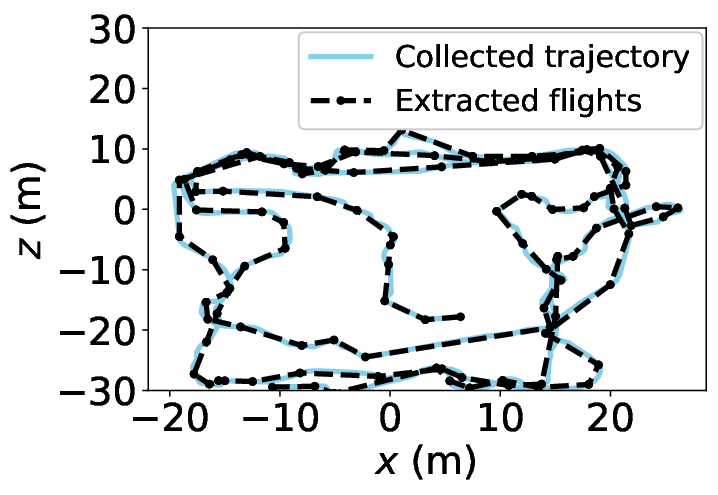


In this section we introduce our model for VR viewport position. We focus on viewport position change over time interval , in order to analyze the ViS of VR frames that are apart.
Adopting the axis notation common in computer graphics [37, 14], the viewport positions in the Earth coordinates (shown in Fig. 2) are denoted as , where is the height of the viewport, and and are the coordinates of the viewport positions in the -plane (i.e., the ground plane). We assume that is constant, e.g., can be set to the human eye level. While changing is important in some specific contexts, such as exergames [38, 39], is fixed in the vast majority of typical VR experiences, and in native Oculus Integration app development, to avoid disorienting the users when they sink below or float above the ground in the virtual environment [40].
To model the change of and , we propose a paused-MRWP position model in the infinite plane, based on our collected pose data and the modified RWP [22]. The model consists of an infinite sequence of points , called waypoints, the pause time at each waypoint, the duration to move along a straight line from to with a constant velocity , and the included angle between and the abscissa. The waypoint is expressed as where and are the coordinates of waypoints in the -plane. The vector is called the -th flight, and is called the direction of the -th flight. At time 0, the viewport is at , and starts to move towards . Due to the constant velocity, the flight time for the -th flight is proportional to its length . The reason for assuming a constant velocity is that although acceleration can be used to produce more realistic movements, constant-velocity VR movement is known to be more comfortable than the movement with acceleration or deceleration [41]. We further assume that , , and are all i.i.d. distributed over . Based on the experimental data in desktop VR, we will propose the models for , , and .
The collected data shows that the viewpoint movement in the -plane is well approximated by a sequence of flights. We apply the standard angle model proposed in [19] to extract flights from the trajectories. Fig. 8 plots the trajectory in -plane of one user in Lite and the extracted flights. Although the viewport does not move in a perfectly straight line during each flight, the trajectory is close to it.
Modeling flight duration. Our experimental data demonstrates that is exponentially distributed, and confirms that the paused-MRWP better models the flight time in VR than the classical RWP models [17]. Specifically, the PDF of the flight times , denoted as , is modeled as . Fig. 8 shows the cumulative distribution function (CDF) of flight times for our collected flight samples, the paused-MRWP model with the best fitted , and the classical RWP with a constant velocity in VK game. We see that the flight times of the paused-MRWP model match the measurements better statistically, with the SSE as low as 0.0021. The exponential distribution with the best fitted will be used to model the flight times in §IV and §V.
Modeling pause time. We model the pause time according to the collected data. Fig. 8 shows that the exponential distribution with a “bump” around zero is a good fit to its distribution. The PDF of the pause times, denoted as , is modeled as , where stands for the PDF of the exponential distribution with parameter , Dirac delta function models the “bump” around zero pause time, and represents the fraction of the “bump”.
Modeling flight direction. From our pose dataset, the flight angles follow the uniform distribution on .
With the developed paused-MRWP model, we will focus on observation intervals of duration , and derive an analytical expression for the moment generating function (MGF) of the displacement between two viewport positions.
Definition 3 (MGF of position displacement).
Consider an observation interval , where is a sample from . Let and be the viewport positions at and , respectively. Then, the position displacement is defined as , and the MGF of , denoted by , is given by .
III-C2 Analysis
In analyzing , there are two mutually exclusive and exhaustive cases to consider. Setting as the auxiliary variables, the Case 1 is the case that , , i.e., we start observing the process when the movement is paused. Let denote the event that Case 1 holds. Let denote the complement of , and is the event that Case 2 holds. The Case 2 is the case that , , i.e., we start observing the process during a flight. We will first obtain the -th () moment of , and , for Cases 1 and 2 in Lemmas 1 and 2. Combined with the probability that Case 1 holds given in Lemma 3, we will obtain in Theorem 1.
Lemma 1.
Assume Case 1 holds. Let , and be the remaining pause duration after in the same pause interval. Let and for . We define the events and as
where and . is the event that we end the observation in a pause interval (, ) and that there are complete flights in . is the event that , and that there are complete flights in . Then, is given by
| (1) |
where
and , with being the confluent hypergeometric function of the first kind.
Proof.
See Appendix References. Proof sketch: Since the collections of events and are mutually disjoint and collectively exhaustive, we write as in (1). To calculate , we express the -th moment of as , where denotes the unit vector whose direction represents the moving direction of the -th flight. Based on the property that is i.i.d. uniformly distributed on and on the distributions of flight and pause times, we get the expressions of . Similar techniques are used to obtain . ∎
Lemma 2.
Assume Case 2 holds. Let , and be the remaining flight duration after in the same flight interval. Let for and for . Let the events and be defined as
where and . Then, is given by
where
Proof.
The proof is similar to that of Lemma 1. ∎
Lemmas 1 and 2 yield the expressions for the -th moment of the position displacement for arbitrary . In VR systems, we analyze the ViS for small . In this case, the number of flights and pauses in the observation interval is limited. The terms of and , , dominate and . a good choice for because the sum of the terms (or ), , accounts for more than 98% of (or ) when s and . Hence, we can simplify the calculation of and by discarding many terms corresponding to the cases of when is small (e.g., s).
Lemma 3.
Let be a sample from and be the probability that falls in a flight interval. Then, exists and is equal to .
Proof.
See Appendix -B. ∎
Theorem 1 (MGF of ).
is given by where is the -th moment of the position displacement and .
Fig. 8 compares the empirical results of the -th moment of , , with the analytical results . We obtain by randomly sampling 5000 pairs of viewport positions that are apart and calculating the position displacement. The gap is smaller than when s and , and is smaller than 6% of in other cases. Theorem 1 will be used to calculate the ViS in §IV.
III-D Correlations between Orientations and Positions
VR viewports’ position and orientation are correlated. Observing the azimuth angles and the walking directions (i.e., the included angle between and the positive direction of X-axis) in our collected data, we find that the azimuth angles fixate around the walking direction. Similar observations have been made about human walking patterns in non-virtual worlds [42, 43]. Supported by the pose data, we assume that the azimuth angle at observation start time is the same as the walking direction.
IV Visibility Similarity
We introduce the model for the average visibility similarity given the viewport-to-content distance () in §IV-A. Then we apply the developed VR pose model to analyze the in §IV-B, and propose the ViS-based VR content splitting algorithm, ALG-ViS, in §IV-C.
IV-A ViS Model
The analytical model for we develop in this section characterizes the statistical average of the inter-frame pixel similarity over different pose changes given the viewport-to-content distance . We define the formally after introducing the camera model to present how viewport pose determines the rendered pixels.
Camera model. In VR, the virtual environment is constructed as computer-generated 3D contents, where the pixels in VR frames are generated by capturing the scenes with the camera. The camera is modeled as a standard pinhole camera following [44]. A 3D point in the virtual environment is projected through the pinhole to a pixel on the VR frame. We denote the camera’s angle of view (AoV) as . In addition, we assume that the far plane of the camera, i.e., the largest viewport-to-content distance beyond which the contents cannot be rendered in the VR frame, is much larger than the viewport position change.
Consider two VR frames generated at and , called reference and novel frames. The cameras that capture these frames are called reference and novel cameras, respectively. A pixel in the reference frame is projected back to the 3D point in the virtual environment, and the 3D point is projected to the corresponding pixel in the novel frame. The viewport-to-content distance is formally defined as the distance between the viewport position of the reference frame and the 3D point. The represents the average similarity of the pixels (of distance ) in the reference frame and their corresponding pixels in the novel frame, where the average is taken over different pose changes of reference and novel frames.
Definition 4 ().
Let denote the number of the reference frame’s pixels that are projected to the 3D points with distance from the reference camera. is expressed as , where , are the positions of the 3D point and the reference camera in the -plane, respectively. Let , , denote the set of the reference frame’s pixels that have the same pixel value as the corresponding pixels in the novel frame. The visibility similarity given is defined as , which is the average percentage of pixels that have the same pixel value as the corresponding pixels in the novel frame among . The mean of is taken over the possible viewport pose changes from reference to novel cameras modeled in §III.

We break down the into two terms: (1) the FoV term , which represents the fraction of the VR contents contained in the FoVs of both the novel and the reference cameras, and (2) the distance term , which quantifies the ratio of the number of pixels representing the same 3D points (of distance ) in the novel and reference frames. In VR systems, the viewport moving closer to the VR contents will result in the use of more pixels to represent the contents. Note that is independent of while is a function of . In our analysis, we ignore the influence of occlusion in , i.e., we do not consider the case where the occluded objects are in the FoV of both reference and novel frames, are rendered in the novel frame, but occluded by the other contents in the reference frame. In our numerical results, we show that their effect is small. We have . The and are defined formally below.
Definition 5 (FoV term).
is defined as the statistical average of the multiplication of the fraction of overlapping polar and azimuth angles of reference and novel cameras.
We analyze with the distributions of and obtained in §III-B. Fig. 9 depicts the positions and angles of reference and novel camera viewports in the -plane. Since the far plane is much larger than , the fraction of the overlapping azimuth angles is . The fraction of the overlapping polar angles is obtained similarly. Hence, the FoV term is
| (2) |
Definition 6 (Distance term).
is defined as
| (3) |
where is the distance between the VR content and the novel camera, and is the included angle between and , as shown in Fig. 9.
IV-B The Analysis of
We first provide a closed-form expression for , and then approximate tightly with a small error.
Theorem 2 (FoV term).
is equal to
where is the scale of the fitted Laplace distribution of , and , where is the PDF of . is equal to
| (4) |
Proof.
See Appendix -C. ∎
We focus on small (e.g., s which belongs to the first case in (4)), as the most relevant, in practice, to exploiting VR frame correlation. In this case, the FoV term only depends on , , and .
Theorem 3 (Distance term).
For , we can approximate within error of , where . Specifically, can be approximated according to
| (5) |
where .
Proof.
From (5), can be approximated by . The approximation error can be made arbitrarily small by choosing a small . is convergent since is bounded by . Hence, is convergent, and the sum of the first terms provides a good approximation with an error in §V.
The time taken to calculate the is dominated by calling the confluent hypergeometric function in Lemmas 1 and 2. The average time, over 100 iterations, for calculating on a Lenovo laptop (equipped with an AMD Ryzen 7 4800H CPU and an NVIDIA GTX 1660 Ti GPU) in MATLAB is only 4.4 ms. Hence, the can be calculated for each frame in real time.
IV-C ViS-Based Foreground and Background Content Splitting
Based on the average ViS for a given , i.e., , we adaptively split the contents to background and foreground, where the background (with a larger ) has a high and can be reused to reduce the resource consumption. To this end, we propose ALG-ViS given in Algorithm 1. For every consecutive frames, the first frame is selected as the reference frame; the remaining frames are the novel frames. In reference frames, all VR contents are classified as foreground contents. In novel frames, we calculate a distance threshold such that , where is the threshold and a larger than indicates high similarity of pixels in reference and novel frames. The VR contents that have the distance from the reference camera are classified as foreground contents, the other contents – as background contents. VR system renders the foreground contents and reuses the pixels for the background contents from the reference frame by view projection [8, 13]. We only need to calculate for values of when the inter-frame interval is fixed (e.g., when the system supports the full frame rate as in §V), which makes ALG-ViS even more lightweight.
V Evaluation


We verify the analysis of ViS via simulations in §V-A and examine the performance of ALG-ViS in real-world VR implementations in §V-B. The parameters are listed in Table V unless otherwise specified.
V-A Examining ViS
V-A1 Simulation settings
| Parameter | Value | Parameter | Value |
|---|---|---|---|
| VR frame resolution | 10801080 | VR frame rate | 60 fps |
| AoV | Mapping scheme | Equiangular | |
| Depth encoding | Linear | Depth map precision | 8 bits |
| Far clipping plane | 50 m | Eye level height | 1.6 m |
| Unity unit: meter | 1:1 | Pairs of viewport poses | 5000 |
We verify the ViS analysis via simulations using Unity Engine 2019.2.14f1 [14] with 3 VR games listed in Table I. The results are analyzed in MATLAB.
To simulate the ViS, we randomly sample 5000 pairs of viewport poses from the collected pose trajectories for reference and novel cameras. We obtain the pristine novel frame rendered by Unity, and the generated novel frame by view projection from the reference frame and its depth map, where each pixel in the depth map represents the distance of the VR contents to the reference camera. Among the generated novel frame’s pixels whose corresponding 3D points are at a distance from the reference camera, the pixels with RGB values with indistinguishable differences from the pristine novel frame constitute the set ; the other pixels form the set . The ViS given is calculated as the proportion of matched pixels . We consider pixel values as indistinguishable when the difference of the pixel values is less than in all RGB channels22 2 is selected as the maximum value such that the structural similarity index measure (SSIM) between the combined and the pristine novel frame is larger than 0.95. The combined novel frame is obtained by replacing the mismatched pixels in the generated novel frame with the corresponding pixels in the pristine novel frame. .
V-A2 Numerical results
Fig. 12 shows the ViS obtained in our simulations, , and the analytically derived ViS, , for headset VR and phone-based VR, for different and . The results for desktop VR are similar to the results for phone-based VR and are omitted. As expected, the ViS declines with (i.e., frames that are separated by a longer time interval are less similar), and increases with (i.e., contents that are farther from the camera change less across different frames). We observe differences between VR interfaces as well: the ViS for headset VR (Fig. 12(a)) is smaller than the ViS for the other interface types (Fig. 12(b)). This is explained by the difference in movement dynamics we observed in our dataset: in headset VR, the users change their viewport orientations and flight directions more rapidly than in the other VR interfaces. Smaller ViS for headset VR implies that fewer VR contents will be classified as background contents. Finally, we note that the gap between the analytical results and the simulations is small, 4.1% on average for m and only 1.6% on average for m. The gap can be attributed to the omission of object occlusions from our analytical derivations. The achieved highly accurate analytical in the high ViS regime (e.g., m) is crucial for selecting the distance threshold to ensure that the background has a high ViS.
The obtained ViS for the three VR games in desktop VR is shown in Fig. 12. The results for the other 2 interface types exhibit the same trends and are omitted. Although VK has a larger number of triangles and vertices, which manifests in higher visual scene complexity, the of VK is larger than the of Office and Lite. This is because users’ pose trajectories in VK have relatively smaller and , and smaller and , corresponding to larger flight lengths and pause durations. In other words, users tend to change both their viewport orientations and positions more slowly in VK. We hypothesize that higher-complexity games may potentially be more engaging, which encourages the users to explore them in a slower, more deliberate fashion. The observed differences between the ViS for different games suggest that it is important to take specific game’s pose characteristics into account.
V-B Performance of ALG-ViS
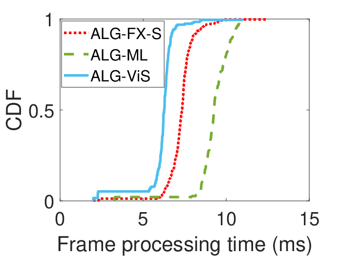
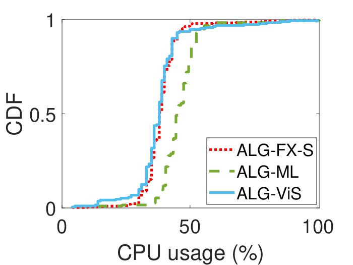
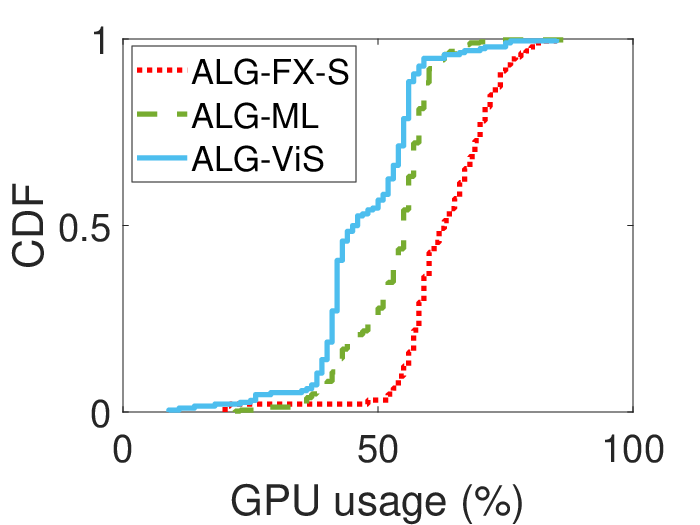
We implement ALG-ViS and a set of baselines in two VR rendering systems, an on-device (“local”) one and one supported by edge computing. Both systems display the generated frames in an Oculus Quest 2 VR headset [45]. On-device rendering system is implemented with build 30.0; its target frame rate is set to the default 72 fps. The edge-assisted system generates the VR frames in a Lenovo laptop, with Unity Engine 2019.1.14f1 and Google VR SDK [46], and sends them to the headset over IEEE 802.11ac WiFi. The laptop is equipped with an AMD Ryzen 7 4800H CPU and an NVIDIA GTX 1660 Ti GPU. The target frame rate of this system is set to the laptop’s default 60 fps. To ensure reproducibility, for all algorithms our evaluation is based on replaying 30 min of headset pose trajectories we collected (see §III-A). We examine the performance for all 3 games, and present the results for Lite, which are representative. We examine the required bandwidth for the edge-supported system in Fig. 12, and the achieved SSIM, frame processing time, and CPU and GPU usage (monitored using the OVR Metrics Tool [47]) for the local system in Fig. 13.
We compare ALG-ViS to different approaches with the same reference frame interval : ALG-FX-S, ALG-FX-T, and ALG-ML. In ALG-ViS, is set to 0.945 to ensure high ViS values for background contents. We set as the minimum integer such that for every frame. In ALG-FX-S and ALG-FX-T, is determined by the number of triangles in the VR frame, similar to the near and far background splitting in [10]. Specifically, , where is fixed for each game. For a fair comparison, in ALG-FX-T, we set to make the average frame processing time of ALG-FX-T and ALG-ViS the same to compare the SSIM; in ALG-FX-S, we set to make the average SSIM the same as ALG-ViS when comparing other metrics. In ALG-ML, we adopt an online ridge regression model, which has been shown to achieve state-of-the-art accuracy in 360∘ video pose prediction [25, 24]. Following [11], we predict , and separately. We set the history and prediction windows as in [11]. We split the VR contents by calculating the ViS of the reference frame and the predicted VR frame.
The CDF of the required bandwidth of the edge-assisted rendering system shown in Fig. 12 demonstrates that ALG-ViS requires less bandwidth on average than ALG-FX-S (11.3% difference; ALG-FX-S consistently transmits more pixels to maintain the same SSIM as ALG-ViS), and has significantly smaller bandwidth variance than ALG-ML (88.4% reduction). Although ALG-ML can save bandwidth when it accurately predicts the viewport pose, the required bandwidth increases drastically when the prediction is erroneous. Generating less bursty traffic, ALG-ViS prevents transmission resource over-provisioning and potential TCP incast problems in edge-assisted VR systems, which helps supporting these systems better when compared with ALG-ML.
Fig. 13 shows the CDFs of the SSIM, frame processing time, and CPU and GPU usage for the local rendering system. It shows that ALG-ViS improves frame quality and frame processing time while consuming fewer resources. The ALG-ViS ensures high average SSIM, outperforming ALG-FX-T by 3.2% and ALG-ML by 5.9%. The ALG-ML exhibits lower frame quality. This is because ALG-ML splits the foreground and background contents based on the predicted pose, and prediction errors lead to severe performance degradation [8]. The ALG-ViS decreases the frame processing time by 16.1% and 33.4% compared to ALG-FX-S and ALG-ML. The CPU usage of ALG-ML is 20.5% higher than that of ALG-ViS due to the extra computation required to tune the regularization parameter and conduct the pose prediction. The GPU usage of ALG-FX-S is 33.7% higher than that of ALG-ViS because ALG-FX-S classifies more VR contents as foreground contents on average. These results demonstrate that the developed ALG-ViS is lightweight yet effective.
VI Conclusion
In this paper, we first propose a viewport pose model for VR systems based on the experimental measurements. We apply the pose model to adaptively select background contents that are reused across VR frames to reduce the communication and computation resource consumption, via quantifying the similarity of pixels across VR frames. Numerical results verify the pose model and the inter-frame pixel similarity analysis. Oculus Quest 2-based implementations of our adaptive background content selection approach show that it improves the image quality by 5.6% and reduces the variance of the required bandwidth by 88.4% compared to the method based on viewport pose prediction.
Acknowledgments
This work is supported in part by NSF grants CSR-1903136, CNS-1908051, and CAREER-2046072, and by an IBM Faculty Award.
References
- [1] S. M. LaValle, Virtual Reality. Cambridge University Press, 2016.
- [2] 3GPP. (2021) Technical specification group services and system aspects; Extended reality (XR) in 5G, TR 26.928 V16.1.0. https://www.3gpp.org/ftp/Specs/archive/26_series/26.928.
- [3] PricewaterhouseCoopers. (2019) Seeing is believing. https://www.pwc.com/seeingisbelieving.
- [4] E. Cuervo, K. Chintalapudi, and M. Kotaru, “Creating the perfect illusion: What will it take to create life-like virtual reality headsets?” in Proc. ACM HotMobile, 2018.
- [5] Z. Tan, Y. Li, Q. Li, Z. Zhang, Z. Li, and S. Lu, “Supporting mobile VR in LTE networks: How close are we?” in Proc. ACM SIGMETRICS, 2018.
- [6] J. Jeong, S. Lee, I. Ryu, T. Le, and E. Ryu, “Towards viewport-dependent 6DoF 360 video tiled streaming for virtual reality systems,” in Proc. ACM MM, 2020.
- [7] L. Liu, R. Zhong, W. Zhang, Y. Liu, J. Zhang, L. Zhang, and M. Gruteser, “Cutting the cord: Designing a high-quality untethered VR system with low latency remote rendering,” in Proc. ACM MobiSys, 2018.
- [8] Y. Li and W. Gao, “DeltaVR: Achieving high-performance mobile VR dynamics through pixel reuse,” in Proc. ACM/IEEE IPSN, 2019.
- [9] Y. Li and W. Gao, “MUVR: Supporting multi-user mobile virtual reality with resource constrained edge cloud,” in Proc. IEEE/ACM SEC, 2018.
- [10] J. Meng, S. Paul, and Y. C. Hu, “Coterie: Exploiting frame similarity to enable high-quality multiplayer VR on commodity mobile devices,” in Proc. ACM ASPLOS, 2020.
- [11] X. Liu, C. Vlachou, F. Qian, C. Wang, and K.-H. Kim, “Firefly: Untethered multi-user VR for commodity mobile devices,” in Proc. USENIX ATC, 2020.
- [12] P. Srivastava, A. Rimzhim, P. Vijay, S. Singh, and S. Chandra, “Desktop VR is better than non-ambulatory HMD VR for spatial learning,” Frontiers Front. Robot. AI, vol. 6, no. 50, pp. 1–15, 2019.
- [13] Y. Liu, J. Liu, A. Argyriou, L. Wang, and Z. Xu, “Rendering-aware VR video caching over multi-cell MEC networks,” IEEE Trans. Veh. Technol., vol. 70, no. 3, pp. 2728–2742, 2021.
- [14] Unity Technologies. (2021) The leading platform for creating interactive, real-time content. [Online]. Available: https://unity.com/
- [15] Z. Lai, Y. C. Hu, Y. Cui, L. Sun, and N. Dai, “Furion: Engineering high-quality immersive virtual reality on today’s mobile devices,” in Proc. ACM MobiCom, 2017.
- [16] I.-H. Hou, N. Z. Naghsh, S. Paul, Y. C. Hu, and A. Eryilmaz, “Predictive scheduling for virtual reality,” in Proc. IEEE INFOCOM, 2020.
- [17] C. Bettstetter, G. Resta, and P. Santi, “The node distribution of the random waypoint mobility model for wireless ad hoc networks,” IEEE Trans. Mobile Comput., vol. 2, no. 3, pp. 257–269, 2003.
- [18] S. Ioannidis and P. Marbach, “A brownian motion model for last encounter routing,” in Proc. IEEE INFOCOM, 2006.
- [19] I. Rhee, M. Shin, S. Hong, K. Lee, and S. Chong, “On the Levy-walk nature of human mobility,” in Proc. IEEE INFOCOM, 2008.
- [20] Y. S. Eroğlu, Y. Yapıcı, and I. Güvenç, “Impact of random receiver orientation on visible light communications channel,” IEEE Trans. Commun., vol. 67, no. 2, pp. 1313–1325, 2019.
- [21] M. D. Soltani, A. A. Purwita, Z. Zeng, H. Haas, and M. Safari, “Modeling the random orientation of mobile devices: Measurement, analysis and LiFi use case,” IEEE Trans. Commun., vol. 67, no. 3, pp. 2157–2172, 2019.
- [22] X. Lin, R. K. Ganti, P. J. Fleming, and J. G. Andrews, “Towards understanding the fundamentals of mobility in cellular networks,” IEEE Trans. Wireless Commun., vol. 12, no. 4, pp. 1686–1698, 2013.
- [23] V. Sitzmann, A. Serrano, A. Pavel, M. Agrawala, D. Gutierrez, B. Masia, and G. Wetzstein, “Saliency in VR: How do people explore virtual environments?” IEEE Trans. Vis. Comput. Graph., vol. 24, no. 4, pp. 1633–1642, 2018.
- [24] F. Qian, B. Han, Q. Xiao, and V. Gopalakrishnan, “Flare: Practical viewport-adaptive 360-degree video streaming for mobile devices,” in Proc. MobiCom, 2018.
- [25] S. Afzal, J. Chen, and K. Ramakrishnan, “Viewing the 360∘ future: Trade-off between user field-of-view prediction, network bandwidth, and delay,” in Proc. IEEE ICCCN, 2020.
- [26] X. Hou and S. Dey, “Motion prediction and pre-rendering at the edge to enable ultra-low latency mobile 6DoF experiences,” IEEE Open J. Commun. Soc., vol. 1, pp. 1674–1690, 2020.
- [27] X. Hou, S. Dey, J. Zhang, and M. Budagavi, “Predictive adaptive streaming to enable mobile 360-degree and VR experiences,” IEEE Trans. Multimedia., vol. 23, pp. 716–731, 2021.
- [28] X. Feng, Z. Bao, and S. Wei, “LiveObj: Object semantics-based viewport prediction for live mobile virtual reality streaming,” IEEE Trans. Vis. Comput. Graphics, vol. 27, no. 5, pp. 2736–2745, 2021.
- [29] E. J. David, J. Gutiérrez, A. Coutrot, M. P. da Silva, and P. L. Callet, “A dataset of head and eye movements for 360∘ videos,” in Proc. ACM MMSys, 2018.
- [30] W. Lo, C. Fan, J. Lee, C. Huang, K. Chen, and C. Hsu, “360∘ video viewing dataset in head-mounted virtual reality,” in Proc. ACM MMSys, 2017.
- [31] J. Chakareski, M. Khan, T. Ropitault, and S. Blandino, “6DOF virtual reality dataset and performance evaluation of millimeter wave vs. free-space-optical indoor communications systems for lifelike mobile VR streaming,” in Proc. IEEE ACSSC, 2020.
- [32] B. Han, Y. Liu, and F. Qian, “ViVo: Visibility-aware mobile volumetric video streaming,” in Proc. ACM MobiCom, 2020.
- [33]
Unity Technologies. (2015) Viking village.
https://assetstore.unity.com/
packages/essentials/tutorial-projects/viking-village-29140. - [34]
Xiaolianhua Studio. (2017) Lite.
https://assetstore.unity.com/packages/
3d/environments/fantasy/make-your-fantasy-game-lite-8312. - [35]
Unity Asset Store. (2020) Office.
https://assetstore.unity.com/packages/
3d/environments/snaps-prototype-office-137490. - [36] B. Everitt and A. Skrondal, The Cambridge dictionary of statistics, 4th ed. Cambridge University Press, 2010.
- [37] E. Lengyel, Foundations of Game Engine Development, Volume 2: Rendering. Terathon Software LLC, 2019.
- [38] Supernatural. (2021) Burn More. Sweat More. Have More Fun. https://www.getsupernatural.com/.
- [39] FITXR. (2021) A new way to exercise. https://fitxr.com/.
- [40]
Oculus for Developers. (2021) Oculus Integration for Unreal Engine basics.
https://developer.oculus.com/documentation/unreal/unreal-engine-
basics/. - [41] L. Terenzi and P. Zaal, “Rotational and translational velocity and acceleration thresholds for the onset of cybersickness in virtual reality,” in Proc. AIAA Scitech Forum, 2020.
- [42] K. A. Turano, D. R. Geruschat, F. H. Baker, J. W. Stahl, and M. D. Shapiro, “Direction of gaze while walking a simple route: Persons with normal vision and persons with retinitis pigmentosa,” Lippincott Williams & Wilkins Optom. Vis. Sci., vol. 78, no. 9, pp. 667–675, 2001.
- [43] M. A. Hollands, A. E. Patla, and J. N. Vickers, ““Look where you’re going!”: Gaze behaviour associated with maintaining and changing the direction of locomotion,” Springer Exp. Brain Res., vol. 143, no. 2, pp. 221–230, 2002.
- [44] R. Tsai, “A versatile camera calibration technique for high-accuracy 3D machine vision metrology using off-the-shelf TV cameras and lenses,” IEEE J. Robot. Autom., vol. 3, no. 4, pp. 323–344, 1987.
- [45] Oculus. (2021) Oculus Quest 2. [Online]. Available: https://www.oculus.com/quest-2/
- [46] Google VR. (2021) Quickstart for Google VR SDK for Unity with Android. https://developers.google.com/vr/develop/unity/get-started- android.
- [47] Oculus. (2021) OVR Metrics Tool. https://developer.oculus.com/ downloads/package/ovr-metrics-tool/.
| (6) | ||||
-A Proof of Lemma 1
When Case 1 holds, there are two possible ways to end the observation interval at time . If , , the observation end time lies in a pause interval. Otherwise, lies in a flight interval. If it lies in a pause interval, the movement includes some number of complete flights without any fractional flights. We do not observe any movement when . For , is the event that lies in a pause interval and there are complete flights in . This leads to the first summation in (1).
If lies in a flight interval, the movement includes some number of complete flights and a fraction of the last flight. is the event that lies in a flight interval and there are complete flights in . This leads to the second summation in (1).
It only remains to calculate and to conclude the proof. We start with . Given , the -th moment of is given by . According to the flight direction model in §III-C, the direction of is i.i.d. uniformly distributed on . Thus, is equal to for and for . Thus, expanding and averaging over , only the terms in which all () have even powers are non-zero. The number of these non-zero terms is . Further, let denote the number of non-zero complete pause intervals (excluding the first and last fractional pause intervals). Denote the set of the non-zero complete pause intervals as . Let be the sum of pause intervals in the observation interval. is given by (6), shown at the top of next page. Using these observations, the expressions for can be obtained similarly, which completes the proof.
-B Proof of Lemma 3
Let be the end time of the -th flight, i.e., . Then, for any , there exists such that , and we can upper and lower bound according to
The lower bound includes an extra pause interval between and by ignoring any possible fractional flight duration. On the other hand, the upper bound includes one complete flight duration between and by ignoring .
When , using Lebesgue’s dominated convergence theorem to replace the order of limit and expectation operators and the law of large numbers (as grows large, tends to infinity), it can be seen that both upper and lower bounds converge to .
-C Proof of Theorem 2
-D Proof of Theorem 3
is uniformly distributed on . This is because the walking direction is the same as (see §III-D), and the included angle of and positive direction of -axis is uniformly distributed on . Taking the average over and substituting , (3) is rewritten as , where is calculated as . We further approximate by with the error . is given as
The approximation error is smaller than , i.e., we have
which concludes the proof.