跳到论文正文
W Papers独立论文阅读器 arXiv:2201.03923 论文正文 计算阅读时间 · 0%
引用这篇论文根据当前论文元数据生成,正式投稿前建议核对。


License: arXiv.org perpetual non-exclusive license
arXiv:2201.03923v2 [math.DS] 02 Jun 2022

Rigorous Computation of Linear Response for intermittent maps

Isaia Nisoli Address: Instituto de Matematica - UFRJ Av. Athos da Silveira Ramos 149, Centro de Tecnologia - Bloco C Cidade Universitaria - Ilha do Fundão. Caixa Postal 68530 21941-909 Rio de Janeiro - RJ - Brasil Email address: nisoli@im.ufrj.br and Toby Taylor-Crush Address: Department of Mathematical Sciences, Loughborough University, Loughborough, Leicestershire, LE11 3TU, UK Email address: T.Taylor-Crush@lboro.ac.uk
Date: August 11, 2026
Abstract.

We present a rigorous numerical scheme for the approximation of the linear response of the invariant density of a map with an indifferent fixed point, with explicit and computed estimates for the error and all the involved constants.

Key words and phrases: 
Linear Response, Intermittent Maps, Transfer Operators, Rigorous Approximations
1991 Mathematics Subject Classification
Primary 37A05, 37E05

1. Introduction

In [38] Ruelle proved that for certain perturbations of uniformly hyperbolic deterministic dynamical systems the underlying SRB measure changes smoothly. He also obtained a formula for the derivative of the SRB measure, called the linear response formula [38]11 1 See also earlier related work [29]. See also [24] for a comprehensive historical account including literature from physics.. Since then, the topic of linear response has been a very active direction of research in smooth ergodic theory. Indeed, the work of Ruelle was refined in the uniformly hyperbolic setting [12, 25], extended to the partially hyperbolic setting [15], and has been a topic of deep investigation for unimodal maps, see [8], the survey article [7], the recent works [3, 9, 14, 39] and references therein. More recently, the topic of linear response was also studied in the context of random or extended systems [6, 16, 18, 23, 31, 40, 44]. Optimisation of statistichal properties through linear respone was develope in [1, 2, 22, 30].

Numerical algorithms for the approximation of linear response for uniformly expanding maps, via finite rank transfer operators was obtain in [4] and via dynamical determinants and periodic orbits in [37]22 2 See also [28] for related work on dynamical determinants., and for uniformly hyperbolic systems [26, 35, 36].

Our work extends the methods in [4] to intermittent maps far from the boundary, allowing us to compute the linear response for LSV maps, a version of the Manneville-Pomeau family, [34] as the exponent at the indifferent fixed point changes.

Linear response for indifferent fixed point maps has been investigated in [5, 10, 32], but three important questions have to be addressed to obtain a rigorous numerical approximation scheme:

  1. (1)

    how to approximate efficiently the involved discretized operators;

  2. (2)

    how to bound the approximation errors involved in the discretization;

  3. (3)

    how to bound explicitly and efficiently the constants used in the proofs of [5, 10, 32].

In our paper we provide answers to the three questions above for general intermittent maps and present an explicit computation for LSV type maps. Our scheme and tecniques are very flexible and can be easily adapted to other one dimensional nonuniformly expanding maps whose associated transfer operators do not admit a spectral gap (or a uniform spectral gap) as long as the linear response formula can be obtained via inducing with the first return map.

In the text are presented some numerical remarks, that allow the reader to get an overview of some of the delicate points of the implementation.

The paper is divided as follows: in Section 2 we state the hypothesis on the dynamical system and state our results, in Section 3 we present the theory behind the approximation of the density for the induced map, in Section 4 we discuss the approximation of the linear response for the induced map, in Section 5 we discuss pulling back the measure to the original map and normalizing the density, in Section 6 we give a proof of the fact that the error may be made as small as wanted, in Section 7 we compute an approximation with an explicit error of the linear response for an LSV map; section 8 is devoted to computing effective bounds for the constants in [5, 32] and section 9 explains the tecnique we use to compute some of the functions involved in our approximation.

Acknowledgements

The authors would like to thank Prof. Bahsoun and Prof. Galatolo for their guidance and assistance, their patience and attention. Isaia Nisoli was partially supported by CNPq, UFRJ, CAPES (through the programs PROEX and the CAPES-STINT project “Contemporary topics in non uniformly hyperbolic dynamics”) and Hokkaido University.

Data Availability

The package used for the computations may be found at https://github.com/orkolorko/InvariantMeasures.jl. The Jupyter notebook with the experiment can be provided under inquiry and will published online as soon as possible.

2. Hypothesis on the map and statement of the results

We are interested in approximating the invariant density and linear response for one dimensional interval maps with an indeterminate fixed point by inducing. In particular we wish to gain explicitly calculable error bounds in the L1L^{1} norm. We use an induced map on [0.5,1][0.5,1], to gain a map with good statistical properties to approximate an invariant density and linear response, and then using a formula used in [5] to pull back our approximation to the invariant density and linear response of the full map. We apply this method to a family of Pomeau-Manneville maps to gain an approximation of the statistics with explicit error.

2.1. Interval maps with an inducing scheme

We introduce now a class (family) of interval maps which are non-uniformly expanding with two branches, for which one can construct an inducing scheme which allow it to inherit the linear response formula from the one for the induced system.

  • •

    Let VV be a neighbourhood of 00. For any ϵ∈V\epsilon\in V, Tϵ:[0,1]→[0,1]T_{\epsilon}\colon[0,1]\to[0,1] is a non-singular map, with respect to Lebesgue measure, mm, with two onto branches T0,ϵ:[0,0.5]→[0,1]T_{0,\epsilon}\colon[0,0.5]\to[0,1] and T1,ϵ:[0.5,1]→[0,1]T_{1,\epsilon}\colon[0.5,1]\to[0,1]. The inverse branches of T0,ϵT_{0,\epsilon}, T1,ϵT_{1,\epsilon} are respectively denoted by g0,ϵg_{0,\epsilon} and g1,ϵg_{1,\epsilon}. We call T0:=TT_{0}:=T the unperturbed map, and TϵT_{\epsilon}, for ϵ≠0\epsilon\not=0, the perturbed map.

  • •

    We assume that for each i=0,1i=0,1 and j=0,1,2j=0,1,2 the following partial derivatives exist and satisfy the commutation relation

    (2.1) ∂ϵgi,ϵ(j)=(∂ϵgi,ϵ)(j).\partial_{\epsilon}g_{i,\epsilon}^{(j)}=(\partial_{\epsilon}g_{i,\epsilon})^{(j)}.
  • •

    We assume that TϵT_{\epsilon} has a unique absolutely continuous invariant measure33 3 The TϵT_{\epsilon} absolutely continuous invariant measure is not assumed to be probabilistic; we allow for TϵT_{\epsilon} to admit a σ\sigma-finite absolutely continuous invariant measure. (up to multiplication) whose Radon-Nikodym derivative will be denoted by hϵh_{\epsilon}, and we denote for simplicity h=h0h=h_{0}.

  • •

    Let T^ϵ\hat{T}_{\epsilon}, be the first return map of TϵT_{\epsilon} to Δ\Delta, where Δ:=[0.5,1]\Delta:=[0.5,1]; i.e., for x∈Δx\in\Delta

    T^ϵ​(x)=TϵRϵ​(x)​(x),\hat{T}_{\epsilon}(x)=T_{\epsilon}^{R_{\epsilon}(x)}(x),

    where

    Rϵ​(x)=inf{n≥1:Tϵn​(x)∈Δ}.R_{\epsilon}(x)=\inf\{n\geq 1:\,T^{n}_{\epsilon}(x)\in\Delta\}.

    We assume that T^ϵ\hat{T}_{\epsilon} has a unique absolutely continuous invariant measure (up to multiplication) with a continuous density denoted h^ϵ∈C0\hat{h}_{\epsilon}\in C^{0}.

  • •

    Let Ω\Omega be the set of finite sequences of the form ω=10n\omega=10^{n}, for n∈ℕ∪{0}n\in\mathbb{N}\cup\{0\}. We set gω,ϵ=g1,ϵ∘g0,ϵng_{\omega,\epsilon}=g_{1,\epsilon}\circ g_{0,\epsilon}^{n}. Then for x∈[0,1]x\in[0,1] we have Tϵn+1∘gω,ϵ​(x)=xT_{\epsilon}^{n+1}\circ g_{\omega,\epsilon}(x)=x. The cylinder sets [ω]ϵ=gω,ϵ​(Δ)[\omega]_{\epsilon}=g_{\omega,\epsilon}(\Delta), form a partition of Δ\Delta (mod 00). For x∈[0,1]x\in[0,1], we assume

    (2.2) supϵ∈Vsupx∈[0,1]|gω,ϵ′​(x)|<∞;\sup_{\epsilon\in V}\sup_{x\in[0,1]}|g^{\prime}_{\omega,\epsilon}(x)|<\infty;
    (2.3) supϵ∈Vsupx∈[0,1]|∂ϵgω,ϵ​(x)|<∞;\sup_{\epsilon\in V}\sup_{x\in[0,1]}|\partial_{\epsilon}g_{\omega,\epsilon}(x)|<\infty;
    (2.4) ∑ωsupϵ∈V‖gω,ϵ′‖ℬ<∞;\sum_{\omega}\sup_{\epsilon\in V}||g^{\prime}_{\omega,\epsilon}||_{\mathcal{B}}<\infty;

    and

    (2.5) ∑ωsupϵ∈V‖∂ϵgω,ϵ′‖ℬ<∞,\sum_{\omega}\sup_{\epsilon\in V}||\partial_{\epsilon}g_{\omega,\epsilon}^{\prime}||_{\mathcal{B}}<\infty,

where ℬ\mathcal{B} denotes the set of continuous functions on (0,1](0,1] with the norm

∥f∥ℬ=supx∈(0,1]|xγf(x)|,\parallel f\parallel_{\mathcal{B}}=\sup\limits_{x\in(0,1]}|x^{\gamma}f(x)|,

for a fixed44 4 In (2.4) and (2.5) we need the assumptions to hold only for a single γ\gamma. γ>0\gamma>0. When equipped with the norm ∥⋅∥ℬ\parallel\cdot\parallel_{\mathcal{B}}, ℬ\mathcal{B} is a Banach space.

For Φ∈L1\Phi\in L^{1}, let

(2.6) Fϵ​(Φ):=1Δ​Φ+(1−1Δ)​∑ω∈ΩΦ∘gω,ϵ​gω,ϵ′.F_{\epsilon}(\Phi):=1_{\Delta}\Phi+(1-1_{\Delta})\sum_{\omega\in\Omega}\Phi\circ g_{\omega,\epsilon}g_{\omega,\epsilon}^{\prime}.

Note that FϵF_{\epsilon} is a linear operator. In fact, for x∈[0,1]∖Δx\in[0,1]\setminus\Delta, the formula of FϵF_{\epsilon} can be re-written using the Perron-Frobenius operator of TϵT_{\epsilon}:

(2.7) Fϵ(Φ):=1ΔΦ+(1−1Δ)∑k≥1Lϵk(Φ⋅1{Rϵ>k}),F_{\epsilon}(\Phi):=1_{\Delta}\Phi+(1-1_{\Delta})\sum_{k\geq 1}L^{k}_{\epsilon}(\Phi\cdot 1_{\{R_{\epsilon}>k\}}),

where LϵL_{\epsilon} is the Perron-Frobenius operator associated with TϵT_{\epsilon}; i.e., for φ∈L∞\varphi\in L^{\infty} and ψ∈L1\psi\in L^{1}

∫φ∘Tϵ⋅ψ​𝑑m=∫φ⋅Lϵ​ψ​𝑑m.\int\varphi\circ T_{\epsilon}\cdot\psi dm=\int\varphi\cdot L_{\epsilon}\psi dm.

It is given in [5] that the densities of the original system and the induced one are related (modulo normalization in the finite measure case) by

(2.8) hϵ=Fϵ​(h^ϵ).h_{\epsilon}=F_{\epsilon}(\hat{h}_{\epsilon}).

We also define the following operator, which represents ∂ϵFϵ​Φ|ϵ=0\partial_{\epsilon}F_{\epsilon}\Phi|_{\epsilon=0}

(2.9) Q​Φ=(1−1Δ)​∑ωΦ′∘gω⋅aω​gω′+Φ∘gω⋅bω,Q\Phi=(1-1_{\Delta})\sum_{\omega}\Phi^{\prime}\circ g_{\omega}\cdot a_{\omega}g_{\omega}^{\prime}+\Phi\circ g_{\omega}\cdot b_{\omega},

where aω=∂ϵgω,ϵ|ϵ=0a_{\omega}=\partial_{\epsilon}g_{\omega,\epsilon}|_{\epsilon=0} and bω=∂ϵgω,ϵ′|ϵ=0b_{\omega}=\partial_{\epsilon}g_{\omega,\epsilon}^{\prime}|_{\epsilon=0}.

2.2. Interval maps with countable number of branches

We introduce here a class of interval maps which are uniformly expanding, with a finite or countable number of branches, for which we will be able to prove a linear response formula. The induced map in Subsection 2.1 is a particular case of such uniformly expanding maps.

Let Δ\Delta be an interval and VV be a neighborhood of 00. Let Ω\Omega be a finite or countable set. We assume that the maps T^ϵ:Δ→Δ\hat{T}_{\epsilon}\colon\Delta\to\Delta satisfy

  • •

    For each ϵ∈V\epsilon\in V, there exists a partition (mod 0) of Δ\Delta into open intervals Δω,ϵ\Delta_{\omega,\epsilon}, ω∈Ω\omega\in\Omega such that the restriction of T^ϵ\hat{T}_{\epsilon} to Δω,ϵ\Delta_{\omega,\epsilon} is piecewise C3C^{3}, onto and uniformly expanding in the sense that infωinfΔω,ϵ|T^ω,ϵ′|>1\inf_{\omega}\inf_{\Delta_{\omega,\epsilon}}|\hat{T}_{\omega,\epsilon}^{\prime}|>1. We denote by gω,ϵg_{\omega,\epsilon} the inverse branches of T^ϵ\hat{T}_{\epsilon} on Δω,ϵ\Delta_{\omega,\epsilon}.

  • •

    We assume that for each ω∈Ω\omega\in\Omega and j=0,1,2j=0,1,2 the following partial derivatives exist and satisfy the commutation relation55 5 Note that (2.10) is satisfied when T^ϵ\hat{T}_{\epsilon} is an induced map as in Subsection 2.1. In particular, for each i=0,1i=0,1 and j=0,1,2j=0,1,2 the following partial derivatives exist and satisfy the commutation relation ∂ϵgi,ϵ(j)=(∂ϵgi,ϵ)(j)\partial_{\epsilon}g_{i,\epsilon}^{(j)}=(\partial_{\epsilon}g_{i,\epsilon})^{(j)}.

    (2.10) ∂ϵgω,ϵ(j)=(∂ϵgω,ϵ)(j).\partial_{\epsilon}g_{\omega,\epsilon}^{(j)}=(\partial_{\epsilon}g_{\omega,\epsilon})^{(j)}.
  • •

    We assume

    (2.11) supωsupϵ∈Vsupx∈Δ|gω,ϵ′′​(x)gω,ϵ′​(x)|<∞;\sup_{\omega}\sup_{\epsilon\in V}\sup_{x\in\Delta}\left|\frac{g_{\omega,\epsilon}^{\prime\prime}(x)}{g_{\omega,\epsilon}^{\prime}(x)}\right|<\infty;

    and for i=2,3i=2,3

    (2.12) ∑ωsupϵ∈Vsupx∈Δ|gω,ϵ(i)​(x)|<∞;\sum_{\omega}\sup_{\epsilon\in V}\sup_{x\in\Delta}|g^{(i)}_{\omega,\epsilon}(x)|<\infty;

    and for i=1,2i=1,2

    (2.13) ∑ωsupϵ∈Vsupx∈Δ|∂ϵgω,ϵ(i)​(x)|<∞.\sum_{\omega}\sup_{\epsilon\in V}\sup_{x\in\Delta}|\partial_{\epsilon}g_{\omega,\epsilon}^{(i)}(x)|<\infty.

Let L^ϵ\hat{L}_{\epsilon} denote the transfer operator of the map T^ϵ\hat{T}_{\epsilon}; i.e., for Φ∈L1​(Δ)\Phi\in L^{1}(\Delta)

L^ϵ​Φ​(x):=∑ω∈ΩΦ∘gω,ϵ​(x)​gω,ϵ′​(x)\hat{L}_{\epsilon}\Phi(x):=\sum_{\omega\in\Omega}\Phi\circ g_{\omega,\epsilon}(x)g_{\omega,\epsilon}^{\prime}(x)

for a.e. x∈Δx\in\Delta. Under these conditions it is well known that T^ϵ\hat{T}_{\epsilon} admits a unique (up to multiplication) finite absolutely continuous invariant measure. We denote its density by h^ϵ\hat{h}_{\epsilon}. Hence L^ϵ​h^ϵ=h^ϵ\hat{L}_{\epsilon}\hat{h}_{\epsilon}=\hat{h}_{\epsilon}. Moreover, L^ϵ\hat{L}_{\epsilon} has a spectral gap when acting on CkC^{k} and Wk,1W^{k,1}, k=1,2k=1,2. We denote the Perron-Frobenius operator of the unperturbed map T^\hat{T} by L^\hat{L}; i.e., L^:=L^0\hat{L}:=\hat{L}_{0} and let h^:=h^0\hat{h}:=\hat{h}_{0}.

2.3. Linear response formula

In [5] it is shown that the invariant density h^ϵ\hat{h}_{\epsilon} of the induced map T^ϵ\hat{T}_{\epsilon} is differentiable as a C0C^{0} element and its linear response formula is given by

(2.14) h^∗:=(I−L^)−1​L^​[A0​h^′+B0​h^],\hat{h}^{*}:=(I-\hat{L})^{-1}\hat{L}[A_{0}\hat{h}^{\prime}+B_{0}\hat{h}],

where h^′\hat{h}^{\prime} is the spatial derivative of h^\hat{h} and

A0=−(∂ϵT^ϵT^ϵ′)|ϵ=0,B0=(∂ϵT^ϵ⋅T^ϵ′′T^ϵ′2−∂ϵT^ϵ′T^ϵ′)|ϵ=0.A_{0}=-\left(\frac{\partial_{\epsilon}\hat{T}_{\epsilon}}{\hat{T}^{\prime}_{\epsilon}}\right){\Big|}_{\epsilon=0},\hskip 14.22636ptB_{0}=\left(\frac{\partial_{\epsilon}\hat{T}_{\epsilon}\cdot\hat{T}_{\epsilon}^{\prime\prime}}{\hat{T}_{\epsilon}^{\prime 2}}-\frac{\partial_{\epsilon}\hat{T}_{\epsilon}^{\prime}}{\hat{T}_{\epsilon}^{\prime}}\right){\Big|}_{\epsilon=0}.

Moreover, for the original map, ϵ↦hϵ\epsilon\mapsto h_{\epsilon} is differentiable as an element of ℬ\mathcal{B}; in particular, if the conditions hold for some γ<1\gamma<1

limϵ→0‖hϵ−hϵ−h∗‖1=0,\lim_{\epsilon\to 0}||\frac{h_{\epsilon}-h}{\epsilon}-h^{*}||_{1}=0,

and h∗h^{*} is given by 66 6 Note that in the finite measure case, h∗h^{*} is the derivative of the non-normalized density hϵh_{\epsilon}. The advantage in working with hϵh_{\epsilon} is reflected in keeping the operator FϵF_{\epsilon} linear and to accommodate the infinite measure preserving case. In the finite measure case, once the derivative of hϵh_{\epsilon} is obtained, the derivative of the normalized density can be easily computed. Indeed, hϵ=h+ϵ​h∗+o⁡(ϵ)h_{\epsilon}=h+\epsilon h^{*}+o(\epsilon). Consequently, ∫hϵ=∫h+ϵ​∫h∗+o⁡(ϵ)\int h_{\epsilon}=\int h+\epsilon\int h^{*}+o(\epsilon). Hence, ∂ϵ(hϵ∫hϵ)|ϵ=0=h∗−h​∫h∗\partial_{\epsilon}(\frac{h_{\epsilon}}{\int h_{\epsilon}}){|}_{\epsilon=0}=h^{*}-h\int h^{*}.

(2.15) h∗=F0​h^∗+Q​h^.h^{*}=F_{0}\hat{h}^{*}+Q\hat{h}.

2.4. Main result and explicit strategy

We focus on the case γ<1\gamma<1. The goal of this work is to provide a numerical scheme that can rigorously approximate h∗h^{*}, up to a pre-specified error τ>0\tau>0, in the L1L^{1}-norm. To obtain such a result we follow the following steps:

  1. (1)

    first provide a sequence of finite rank operators L^η\hat{L}_{\eta} that can be used to approximate the linear response for the induced map h^∗\hat{h}^{*} in L1​(Δ)L^{1}(\Delta). Since the formula of h^∗\hat{h}^{*} involves h^\hat{h} and h^′\hat{h}^{\prime}, we will design L^η\hat{L}_{\eta} so that its invariant density, h^η\hat{h}_{\eta}, well approximates hηh_{\eta} in the C1C^{1}-norm,

  2. (2)

    we pull-back to the original map by defining F0appF_{0}^{\text{app}} and Q0appQ_{0}^{\text{app}} by truncating (2.6) and (2.9); i.e., for Φ∈L1\Phi\in L^{1},

    F0app​(Φ):=1Δ​Φ+(1−1Δ)​∑ω=1N∗Φ∘gω,0​gω,0′F_{0}^{\text{app}}(\Phi):=1_{\Delta}\Phi+(1-1_{\Delta})\sum_{\omega=1}^{N^{*}}\Phi\circ g_{\omega,0}g_{\omega,0}^{\prime}

    and

    Qapp​Φ=(1−1Δ)​∑ω=1N∗Φ′∘gω⋅aω​gω′+Φ∘gω⋅bωQ^{\text{app}}\Phi=(1-1_{\Delta})\sum_{\omega=1}^{N^{*}}\Phi^{\prime}\circ g_{\omega}\cdot a_{\omega}g_{\omega}^{\prime}+\Phi\circ g_{\omega}\cdot b_{\omega}
  3. (3)

    finally, find N∗N^{*} large enough and set

    (2.16) hη∗:=F0app​h^η∗+Qapp​h^ηh^{*}_{\eta}:=F_{0}^{\text{app}}\hat{h}_{\eta}^{*}+Q^{\text{app}}\hat{h}_{\eta}

    so that

    ‖hη∗−h∗‖1≤τ.\|h^{*}_{\eta}-h^{*}\|_{1}\leq\tau.

This strategy allows us to prove the following theorem.

Theorem 2.1.

For any τ>0\tau>0, there exists a sequence of finite rank operators L^η:L1​(Δ)→L1​(Δ)\hat{L}_{\eta}:L^{1}(\Delta)\to L^{1}(\Delta) such that for η>0\eta>0 small enough and N∗>0N^{*}>0 large enough

‖hη∗−h∗‖1≤τ.\|h^{*}_{\eta}-h^{*}\|_{1}\leq\tau.

2.5. The validated numerics toolbox

While the strategy for the approximation of the linear response may seems quite simple, to make it rigorous, i.e., with a certified control on the error terms so that the results have the strength of proofs, many different quantities have to be estimated explictly by means of a priori and a posteriori estimates.

The main toolbox we use for these validated estimates consists in

  1. (1)

    Interval Arithmetics and rigorous contractors as the Interval Newton Method and the Shooting Method [42]

  2. (2)

    discretization of the transfer operator, using the Ulam and Chebyshev basis [20, 19, 43]

  3. (3)

    a priori estimate on the tail of a series and rigorous bounds for a finite number of terms.

We will introduce these methods and some of their implementation details during the proof of our result, showing the difference with the cited references when needed.

3. Approximating the invariant density of the induced map

To approximate the invariant density for the induced map two approximation steps are needed. First we need to approximate the induced map, which has countable branches with a map with a finite number of branches. Then, we will discretize the transfer operator of this map by using a Chebyshev approximation scheme.

3.1. From countable branches to finite branches

Let δk>0\delta_{k}>0 with δk=|∪n=k∞[ω]|\delta_{k}=\left|\cup_{n=k}^{\infty}[\omega]\right|. To simplify notation we assume without loss of generality that 12∈∪n=k∞[ω]¯\frac{1}{2}\in\overline{\cup_{n=k}^{\infty}[\omega]}. Let

T^δk​(x)={T^​(x) , if ​x∈[δk,1],12​δk−1​(x−12)+12 , if ​x∈[0.5,δk).\hat{T}_{\delta_{k}}(x)=\begin{cases}\hat{T}(x)&\mbox{ , if }x\in[\delta_{k},1],\\ \frac{1}{2}\delta_{k}^{-1}(x-\frac{1}{2})+\frac{1}{2}&\mbox{ , if }x\in[0.5,\delta_{k}).\\ \end{cases}

Then the transfer operator L^δk\hat{L}_{\delta_{k}}, associated with TδkT_{\delta_{k}} is acting on Φ∈L1​(Δ)\Phi\in L^{1}(\Delta) as:

L^δk​Φ​(x):=∑n<kω∈ΩΦ∘gω,ϵ​(x)​gω,ϵ′​(x)+Φ⁡(δk​(2​x−1)+12)​2​δk\hat{L}_{\delta_{k}}\Phi(x):=\sum_{\overset{\omega\in\Omega}{n<k}}\Phi\circ g_{\omega,\epsilon}(x)g_{\omega,\epsilon}^{\prime}(x)+\Phi\left(\delta_{k}(2x-1)+\frac{1}{2}\right)2\delta_{k}

for a.e. x∈Δx\in\Delta.

Lemma 3.1.

Let Φ∈C1\Phi\in C^{1}, then

‖(L^−L^δk)​Φ‖C1≤(D+D0​D+2)​‖Φ‖C1​δk,\|(\hat{L}-\hat{L}_{\delta_{k}})\Phi\|_{C^{1}}\leq(D+D_{0}D+2)\|\Phi\|_{C^{1}}\delta_{k},

where D0=‖gω′′gω′‖∞D_{0}=\Big\|\frac{g_{\omega}^{\prime\prime}}{g^{\prime}_{\omega}}\Big\|_{\infty} and D≥2​supω|gω′​(x)||gω′​(y)|D\geq 2\sup_{\omega}\frac{|g^{\prime}_{\omega}(x)|}{|g^{\prime}_{\omega}(y)|} for all77 7 The existence of a uniform constant D>0D>0 is implied by condition (2.11). x,yx,y in [0.5,1][0.5,1].

Proof.

First notice that

(3.1) |(L^−L^δk)​Φ|=|∑n≥kω∈ΩΦ∘gω​(x)​gω′​(x)−Φ⁡(δk​(2​x−1)+12)​2​δk|≤∑n≥kω∈Ω|Φ∘gω​(x)|⋅|gω′​(x)|+|Φ⁡(δk​(2​x−1)+12)|​2​δk\begin{split}\left|(\hat{L}-\hat{L}_{\delta_{k}})\Phi\right|&=\left|\sum_{\overset{\omega\in\Omega}{n\geq k}}\Phi\circ g_{\omega}(x)g_{\omega}^{\prime}(x)-\Phi(\delta_{k}(2x-1)+\frac{1}{2})2\delta_{k}\right|\\ &\leq\sum_{\overset{\omega\in\Omega}{n\geq k}}|\Phi\circ g_{\omega}(x)|\cdot|g_{\omega}^{\prime}(x)|+|\Phi(\delta_{k}(2x-1)+\frac{1}{2})|2\delta_{k}\end{split}

and

(3.2) |((L^−L^δk)​Φ)′|=|∑n≥kω∈Ω(Φ′∘gω​(x)​(gω′​(x))2+Φ∘gω​(x)​gω′′​(x))−|Φ′​(δk​(2​x−1)+12)​4​δk2||≤∑n≥kω∈Ω|Φ′∘gω​(x)|⋅(gω′​(x))2+supω‖gω′′gω′‖∞​∑n≥kω∈Ω|Φ∘gω​(x)|⋅|gω′​(x)|+|Φ′​(δk​(2​x−1)+12)|​4​δk2.\begin{split}&\left|\left((\hat{L}-\hat{L}_{\delta_{k}})\Phi\right)^{\prime}\right|=\\ &\left|\sum_{\overset{\omega\in\Omega}{n\geq k}}\left(\Phi^{\prime}\circ g_{\omega}(x)(g_{\omega}^{\prime}(x))^{2}+\Phi\circ g_{\omega}(x)g_{\omega}^{\prime\prime}(x)\right)\right.\left.-|\Phi^{\prime}(\delta_{k}(2x-1)+\frac{1}{2})4\delta_{k}^{2}|\right|\\ &\leq\sum_{\overset{\omega\in\Omega}{n\geq k}}|\Phi^{\prime}\circ g_{\omega}(x)|\cdot(g_{\omega}^{\prime}(x))^{2}+\sup_{\omega}\Big\|\frac{g_{\omega}^{\prime\prime}}{g^{\prime}_{\omega}}\Big\|_{\infty}\sum_{\overset{\omega\in\Omega}{n\geq k}}|\Phi\circ g_{\omega}(x)|\cdot|g_{\omega}^{\prime}(x)|\\ &+|\Phi^{\prime}(\delta_{k}(2x-1)+\frac{1}{2})|4\delta_{k}^{2}.\end{split}

Now notice that by the Mean Value Theorem, ∃ξω∈(12,1)\exists\,\xi_{\omega}\in(\frac{1}{2},1) such that

|gω​(1)−gω​(12)|=|gω′​(ξω)|/2.|g_{\omega}(1)-g_{\omega}(\frac{1}{2})|=|g^{\prime}_{\omega}(\xi_{\omega})|/2.

Therefore,

(3.3) |gω′​(x)|≤2​|gω​(1)−gω​(12)|⋅supω|gω′​(x)||gω′​(ξω)|:=D⋅|gω​(1)−gω​(12)|.|g^{\prime}_{\omega}(x)|\leq 2|g_{\omega}(1)-g_{\omega}(\frac{1}{2})|\cdot\sup_{\omega}\frac{|g^{\prime}_{\omega}(x)|}{|g^{\prime}_{\omega}(\xi_{\omega})|}:=D\cdot|g_{\omega}(1)-g_{\omega}(\frac{1}{2})|.

Thus, using (3.3) in (3.1) and (3.2), we obtain

(3.4) |(L^−L^δk)​Φ|+|((L^−L^δk)​Φ)′|≤‖Φ‖C0​D​∑n≥kω∈Ω|gω​(1)−gω​(12)|+‖Φ‖C0​2​δk+(∥Φ′∥C0D+∥Φ∥C0Dsupω∥gω′′gω′∥∞)∑n≥kω∈Ω⋅|gω(1)−gω(12)|+∥Φ′∥C04δk2=(D+D0​D+2)​‖Φ‖C0​δk+‖Φ′‖C0​4​δk2≤(D+D0​D+2)​‖Φ‖C1​δk.\begin{split}&\left|(\hat{L}-\hat{L}_{\delta_{k}})\Phi\right|+\left|\left((\hat{L}-\hat{L}_{\delta_{k}})\Phi\right)^{\prime}\right|\leq\|\Phi\|_{C^{0}}D\sum_{\overset{\omega\in\Omega}{n\geq k}}|g_{\omega}(1)-g_{\omega}(\frac{1}{2})|+\|\Phi\|_{C^{0}}2\delta_{k}\\ &\hskip 14.22636pt+\left(\|\Phi^{\prime}\|_{C^{0}}D+\|\Phi\|_{C^{0}}D\sup_{\omega}\Big\|\frac{g_{\omega}^{\prime\prime}}{g^{\prime}_{\omega}}\Big\|_{\infty}\right)\sum_{\overset{\omega\in\Omega}{n\geq k}}\cdot|g_{\omega}(1)-g_{\omega}(\frac{1}{2})|+\|\Phi^{\prime}\|_{C^{0}}4\delta_{k}^{2}\\ &\hskip 14.22636pt=(D+D_{0}D+2)\|\Phi\|_{C^{0}}\delta_{k}+\|\Phi^{\prime}\|_{C^{0}}4\delta_{k}^{2}\leq(D+D_{0}D+2)\|\Phi\|_{C^{1}}\delta_{k}.\end{split}

∎

The next lemma shows that using the above information, the densities h^\hat{h} and h^δk\hat{h}_{\delta_{k}} can be made arbitrarily close in C1C^{1}.

Lemma 3.2.

For two operators, L1L_{1} and L2L_{2}, with fixed points h1h_{1} and h2h_{2} normalised with respect to ||⋅||1||\cdot||_{1}, and a shared Lasota-Yorke innequality

‖Lin​f‖s≤A​λn​‖f‖s+B​‖f‖w\left\lVert L_{i}^{n}f\right\rVert_{s}\leq A\lambda^{n}\left\lVert f\right\rVert_{s}+B\left\lVert f\right\rVert_{w}

for i∈{1,2}i\in\{1,2\}, there is a C∗C^{*} such that ‖Lin​f‖s≤C∗​‖f‖s\left\lVert L_{i}^{n}f\right\rVert_{s}\leq C^{*}\left\lVert f\right\rVert_{s}, and for any N≥1N\geq 1 we have

‖h1−h2‖s≤‖L1N​(h1−h2)‖s+N​C∗||(L1−L2)​h2||s.||h_{1}-h_{2}||_{s}\leq||L_{1}^{N}(h_{1}-h_{2})||_{s}+NC^{*}||(L_{1}-L_{2})h_{2}||_{s}.

Furthermore if ‖L1N|U0‖s≤CN<1\left\lVert L_{1}^{N}|_{U^{0}}\right\rVert_{s}\leq C_{N}<1 then we can have

‖h1−h2‖s≤N​C∗​‖(L1−L2)​h2‖s1−CN.||h_{1}-h_{2}||_{s}\leq\frac{NC^{*}||(L_{1}-L_{2})h_{2}||_{s}}{1-C_{N}}.
Proof.

The value of C∗C^{*} is given by A​λ+BA\lambda+B, and the distance between the two fixed points is shown as follows,

‖h1−h2‖s\displaystyle||h_{1}-h_{2}||_{s} ≤\displaystyle\leq ‖L1N​h1−L2N​h2‖s\displaystyle||L_{1}^{N}h_{1}-L_{2}^{N}h_{2}||_{s}
≤\displaystyle\leq ‖L1N​(h1−h2)‖s+‖(L1N−L2N)​h2‖s.\displaystyle||L_{1}^{N}(h_{1}-h_{2})||_{s}+||(L_{1}^{N}-L_{2}^{N})h_{2}||_{s}.

Note that

(L1N−L2N)​h2\displaystyle(L_{1}^{N}-L_{2}^{N})h_{2} =\displaystyle= ∑k=1NL1N−k​(L1−L2)​L2k−1​h2\displaystyle\sum_{k=1}^{N}L_{1}^{N-k}(L_{1}-L_{2})L_{2}^{k-1}h_{2}
=\displaystyle= ∑k=1NL1N−k​(L1−L2)​h2.\displaystyle\sum_{k=1}^{N}L_{1}^{N-k}(L_{1}-L_{2})h_{2}.

Consequently,

‖(L1N−L2N)​h2‖s\displaystyle||(L_{1}^{N}-L_{2}^{N})h_{2}||_{s} ≤\displaystyle\leq ∑k=1NC∗​‖(L1−L2)​h2‖s\displaystyle\sum_{k=1}^{N}C^{*}||(L_{1}-L_{2})h_{2}||_{s}
≤\displaystyle\leq N​C∗​‖(L1−L2)​h2‖s.\displaystyle NC^{*}||(L_{1}-L_{2})h_{2}||_{s}.

Given that ‖h1‖1=‖h2‖1||h_{1}||_{1}=||h_{2}||_{1} we have that h1−h2∈U0h_{1}-h_{2}\in U^{0} and therefore we can bound ‖L1N​(h1−h2)‖s||L_{1}^{N}(h_{1}-h_{2})||_{s} by CN​‖h1−h2‖sC_{N}||h_{1}-h_{2}||_{s}, rearranging gives us the last result. ∎

Remark 3.3.

The operators L^\hat{L} and L^δk\hat{L}_{\delta_{k}} admit a uniform Lasota-Yorke inequality,

‖L^n​f‖C1≤A​λn​‖f‖C1+B​‖f‖C0\left\lVert\hat{L}^{n}f\right\rVert_{C^{1}}\leq A\lambda^{n}\left\lVert f\right\rVert_{C^{1}}+B\left\lVert f\right\rVert_{C^{0}}

as shown in section 8.2.1, where a value for C∗C^{*} is found. Bounds on ‖Lδk|U0‖C1\left\lVert L_{\delta_{k}}|_{U^{0}}\right\rVert_{C^{1}} can be found by techniques described in section 3.2.4. The C1C^{1} norms of h^δk\hat{h}_{\delta_{k}} and h^\hat{h} can be estimated using the Lasota-Yorke inequalities. We can then use lemma 3.1 to make the error in ‖h^δk−h^‖C1||\hat{h}_{\delta_{k}}-\hat{h}||_{C^{1}} as small as we like.

Next we define a finite rank operator to obtain h^n\hat{h}_{n} so that ‖h^n−h^δk‖C1\|\hat{h}_{n}-\hat{h}_{\delta_{k}}\|_{C^{1}} can be made as small as required.

3.2. Approximating the invariant density for T^δk\hat{T}_{\delta_{k}}

To approximate the invariant density, we will discretize the operator L^δk\hat{L}_{\delta_{k}} using the basis of the Chebyshev polynomials of the first kind. The Chebyshev basis is a basis for the space of polynomials with a main advantage: given a continuous function ff on [−1,1][-1,1] the interpolating polynomial on the Chebyshev points are “near-best” approximants with respect to ||.||∞||.||_{\infty} [41, Theorem 16.1]; moreover if the function ff is regular enough the coefficients of the interpolant decay “fast” and are easily computed by means of the Fast Fourier Transform.

Before going forward, some observations are in order, since Chebyshev polynomials do not solve all the problems involved with approximation: to apply this approximation scheme we need to prove a priori that our stationary density is regular enough and keep track of all the errors involved in the computation of the coefficients. Moreover, evaluating a Chebyshev polynomial of high degree rigorously is a delicate matter [33].

3.2.1. Chebyshev interpolation and projection

The material for this section comes from [41], [27] and [45].

Given an f∈Wk,pf\in W^{k,p} from [−1,1]→ℂ[-1,1]\to\mathbb{C}, we can define a function ℱ⁡(θ)\mathcal{F}(\theta) on [0,2​π][0,2\pi] by

ℱ⁡(θ)=f⁡(cos⁡(θ)).\mathcal{F}(\theta)=f(\cos(\theta)).

The Fast Fourier Transform (FFT) on a grid of size 2​N2N allows us to compute the coefficients aka_{k} of the trigonometric polynomial interpolating ℱ\mathcal{F} on an equispaced grid θi=(2​π​i)/(2​N)\theta_{i}=(2\pi i)/(2N), for ii in 0,…,2​N−10,\ldots,2N-1.

Let xi=cos⁡(θi)x_{i}=\cos(\theta_{i}) for ii in 1,…,N1,\ldots,N; observe that ℱ⁡(θi)=ℱ⁡(θ2​N−i)=f⁡(xi)\mathcal{F}(\theta_{i})=\mathcal{F}(\theta_{2N-i})=f(x_{i}). We define the Chebyshev polynomials by the relation

Tn​(cos⁡(θ))=cos⁡(n​θ),T_{n}(\cos(\theta))=\cos(n\theta),

then, if we denote by b0=a0/2b_{0}=a_{0}/2, bN−1=aN−1/2b_{N-1}=a_{N-1}/2 and bi=aib_{i}=a_{i} for all i=1,…,N−2i=1,\ldots,N-2:

p⁡(x)=∑k=0N−1bk​Tk​(x),p(x)=\sum_{k=0}^{N-1}b_{k}T_{k}(x),

where the aka_{k} are the ones computed by the FFT is the interpolating polynomial of ff on the grid given by the xix_{i}.

Definition 3.4.

Let f∈Wk,1f\in W^{k,1}, k>1k>1, we define the Chebyshev (interpolating) projection

πn​f=∑k=0nak​Tk​(x).\pi_{n}f=\sum_{k=0}^{n}a_{k}T_{k}(x).
Remark 3.5.

If, instead of the FFT we had taken the Fourier transform of ℱ\mathcal{F}, the Fourier coefficients a^k\hat{a}_{k} would define coefficients b^k\hat{b}_{k}, the Chebyshev orthogonal expansion

f⁡(x)=∑k=0+∞b^k​Tk​(x),f(x)=\sum_{k=0}^{+\infty}\hat{b}_{k}T_{k}(x),

and the Chebyshev projection

π^n​f=∑k=0nb^k​Tk​(x).\hat{\pi}_{n}f=\sum_{k=0}^{n}\hat{b}_{k}T_{k}(x).

The coefficients aka_{k} and a^k\hat{a}_{k} are related by the aliasing relation:

ak=∑p∈ℤa^k+p​2​n,a_{k}=\sum_{p\in\mathbb{Z}}\hat{a}_{k+p2n},

a-priori knowledge of the regularity of ff allows to estimate the aliasing error above.

This foundational Theorem from [41] estimates the decay rate of the Chebyshev coefficients.

Theorem 3.6.

For an integer ν≥0\nu\geq 0, let ff and its derivatives through f(ν−1)f^{(\nu-1)} be absolutely continuous on [−1,1][-1,1] and suppose the νt​h\nu^{th} derivative f(ν)f^{(\nu)} is of bounded variation VV. Then for k≥ν+1k\geq\nu+1, the Chebyshev coefficients of ff satisfy

|b^k|≤2​Vπ​k​(k−1)​…​(k−ν)≤2​Vπ​(k−ν)ν+1.|\hat{b}_{k}|\leq\frac{2V}{\pi k(k-1)\dots(k-\nu)}\leq\frac{2V}{\pi(k-\nu)^{\nu+1}}.

The decay rate of Chebyshev coefficients allows us to estimate the projection error in C0C^{0} and C1C^{1} norm.

Theorem 3.7.

If ff satisfies the conditions of Theorem 3.6, with VV again the total variation of f(ν)f^{(\nu)} for some ν≥1\nu\geq 1, then for any n≥νn\geq\nu, its Chebyshev projection satisfies

‖f−πn​f‖∞≤2​Vπ​ν​n​(n−1)​…​(n+1−ν)\left\lVert f-\pi_{n}f\right\rVert_{\infty}\leq\frac{2V}{\pi\nu n(n-1)\dots(n+1-\nu)}

The following theorem is a consequence of combining theorem 3.6, with the proof of theorem 2.3 from [45],

Theorem 3.8.

If f,f′,…,f(ν−1)f,f^{\prime},\dots,f^{(\nu-1)} are absolutely continuous on [−1,1][-1,1] and if ‖f(ν)‖1=V<∞\left\lVert f^{(\nu)}\right\rVert_{1}=V<\infty for some ν≥0\nu\geq 0, then for each n≥ν+1n\geq\nu+1, we have that for ν>2\nu>2

‖f′−(πn​f)′‖∞≤4​(n+1)​Vn⁡(ν−2)​π​(n−2)​(n−3)​…​(n+1−ν).\left\lVert f^{\prime}-(\pi_{n}f)^{\prime}\right\rVert_{\infty}\leq\frac{4(n+1)V}{n(\nu-2)\pi(n-2)(n-3)\dots(n+1-\nu)}.
Proof.

From the proof of theorem 2.3 from [45] we have

‖f′−(πn​f)′‖∞≤2​∑k=n+1∞|ak|​k2\left\lVert f^{\prime}-(\pi_{n}f)^{\prime}\right\rVert_{\infty}\leq 2\sum_{k=n+1}^{\infty}|a_{k}|k^{2}

and theorem 3.6 then gives

‖f′−(πn​f)′‖∞≤\displaystyle\left\lVert f^{\prime}-(\pi_{n}f)^{\prime}\right\rVert_{\infty}\leq ∑k=n+1∞4​V​k2π​k​(k−1)​…​(k−ν)\displaystyle\sum_{k=n+1}^{\infty}\frac{4Vk^{2}}{\pi k(k-1)\dots(k-\nu)}
≤\displaystyle\leq 4​(n+1)​Vn⁡(k−2)​π​(n−2)​(n−3)​…​(n+1−k).\displaystyle\frac{4(n+1)V}{n(k-2)\pi(n-2)(n-3)\dots(n+1-k)}.

∎

We can use these theorems to bound the error of Chebyshev projections in the C1C_{1} norm.

3.2.2. Numerical remarks: FFT and Chebyshev

It is important to have an explicit estimate of the error on the coefficients introduced by the FFT. The main issue here is that, when we computing Chebyshev points and evaluating the function ff are not exact operation. To compute rigorous inclusions of the true mathematical value, we use Interval Arithmetics [42].

This means that we need to compute the FFT of a vector of intervals, not of floating point numbers. The following is the consequence of a classical result from [27] that allows us to find a vector of intervals that encloses the Fast Fourier Transform of any element of the vector of the values. This allows us to use optimized implementations of the FFT algorithm as FFTW [17].

Lemma 3.9.

Let f~\tilde{f} be a vector of intervals of dimension N, fmf_{m} the vector of their midpoints, frf_{r} the vector of their radiuses. Let a^\hat{a} be the computed FFT of fmf_{m}. Then

‖a^−a¯‖2≤log2⁡(N)N​(η1−η​‖fm‖2+‖fr‖2).\left\lVert\hat{a}-\bar{a}\right\rVert_{2}\leq\frac{\log_{2}(N)}{\sqrt{N}}(\frac{\eta}{1-\eta}\left\lVert f_{m}\right\rVert_{2}+\left\lVert f_{r}\right\rVert_{2}).

where a¯\bar{a} is the exact FFT for any f∈f~f\in\tilde{f}, η=μ+γ4​(2+μ)\eta=\mu+\gamma_{4}(\sqrt{2}+\mu) with μ\mu the absolute error in the computation of the twiddle factors and γ4=4​u/(1−4​u)\gamma_{4}=4u/(1-4u) where uu is the unit roundoff.

3.2.3. Bounding the error on the invariant density

Let πn\pi_{n} be the Chebyshev projection and let

L^η=πn​L^δk​πn\hat{L}_{\eta}=\pi_{n}\hat{L}_{\delta_{k}}\pi_{n}

be our finite rank approximation of L^δk\hat{L}_{\delta_{k}}.

Lemma 3.10.

If 1/T^δk1/\hat{T}_{\delta_{k}} is of class CνC^{\nu} then L^δk\hat{L}_{\delta_{k}} admits Lasota-Yorke like inequalities of the form

‖(L^δkn​f)(k)‖1≤(λk)n​‖f(k)‖1+A~k​‖f‖Wk−1,1,\left\lVert(\hat{L}_{\delta_{k}}^{n}f)^{(k)}\right\rVert_{1}\leq(\lambda^{k})^{n}\left\lVert f^{(k)}\right\rVert_{1}+\tilde{A}_{k}\left\lVert f\right\rVert_{W^{k-1,1}},

for some ν∈ℕ\nu\in\mathbb{N} for k=1,…,νk=1,\dots,\nu. This implies that if hδkh_{\delta_{k}} is a fixed point of L^δk\hat{L}_{\delta_{k}}

‖hδk‖Wk,1≤Ak1−λk​‖hδk‖Wk−1,1||h_{\delta_{k}}||_{W^{k,1}}\leq\frac{A_{k}}{1-\lambda^{k}}||h_{\delta_{k}}||_{W^{k-1,1}}
Remark 3.11.

The Lasota-Yorke inequalities give us an upper bound on the Wk,1W^{k,1} norm of the fixed point. This, together with Theorems 3.7 and 3.8 permit us to control the discretization error. To estimate our error, we need to compute the constants of this Lasota-Yorke inequality explicitly, we refer to Subsection 7.2.3 for the tecnique we used.

Remark 3.12.

We can use theorems 3.7 and 3.8, together with lemma 3.10 to get a bound on ‖L^δk−L^n‖C1||\hat{L}_{\delta_{k}}-\hat{L}_{n}||_{C^{1}} and the techniques from section 3.2.4 to with lemma 3.2 using operators L^δk\hat{L}_{\delta_{k}} and L^n\hat{L}_{n} in order to bound ‖h^δk−h^n‖C1\left\lVert\hat{h}_{\delta_{k}}-\hat{h}_{n}\right\rVert_{C^{1}} explicitly.

This approach is now quite established, a full treatment can be found in [20, 19].

Remark 3.13.

The discretized operator obtained by the Chebyshev discretization does not preserve the value of the integral. To solve this issue, as in [19] we correct the behaviour of the discretized operator by defining a new operator

Q^n​f=L^n​f+1⋅(∫f​𝑑x−∫L^n​f​𝑑x)\hat{Q}_{n}f=\hat{L}_{n}f+1\cdot(\int fdx-\int\hat{L}_{n}fdx)

which is guaranteed to preserve the space of average 00 measure and has eigenvalue 11, since the row vector that contains the integrals of the basis elements is preserved by multiplication on the left.

3.2.4. Numerical remarks: convergence rates

The problem of bounding the error in C1C^{1} is now reduced to estimate cNc_{N} such that ‖L^nN|U0‖C1≤cN\left\lVert\hat{L}_{n}^{N}|_{U^{0}}\right\rVert_{C^{1}}\leq c_{N}. Since the operator LnL_{n} is of finite rank, we can use numerical methods to compute these quantities in a rigorous way.

Given a basis {ei}i\{e_{i}\}_{i} of U0U^{0} normalized with respect to the C1C^{1} norm, a generic function vv in U0U^{0} is written as v=∑i=1Nbi​eiv=\sum_{i=1}^{N}b_{i}e_{i}. We want to find a constants CkC_{k} such that

‖L^nk​v‖C1≤Ck​‖v‖C1.||\hat{L}_{n}^{k}v||_{C^{1}}\leq C_{k}||v||_{C^{1}}.

If a ckc_{k} exists such that for all basis elements eie_{i} we have

‖L^nk​ei‖C1≤ck.||\hat{L}_{n}^{k}e_{i}||_{C^{1}}\leq c_{k}.

then

‖L^nk​v‖C1≤ck​∑i=1N|bi|≤ck​‖b‖ℓ1||\hat{L}_{n}^{k}v||_{C^{1}}\leq c_{k}\sum_{i=1}^{N}|b_{i}|\leq c_{k}||b||_{\ell^{1}}

where the ℓ1\ell_{1} norm is the linear algebra norm on the coefficients; we will exhibit a constant DD such that ||.||ℓ1≤D||.||C1||.||_{\ell^{1}}\leq D||.||_{C^{1}}; then Ck≤D​ckC_{k}\leq Dc_{k}.

A basis of U0U^{0} in the Chebyshev basis is given by

ei=\displaystyle e_{i}= gi‖gi‖C1,wheregi​(x)=Ti​(x)−∫−11Ti​(x)​𝑑x.\displaystyle\frac{g_{i}}{\left\lVert g_{i}\right\rVert_{C^{1}}},\quad\textrm{where}\quad g_{i}(x)=T_{i}(x)-\int_{-1}^{1}T_{i}(x)dx.

We can link the Chebyshev coefficients aia_{i} and bib_{i} by

a0=−∑i=1Nbi∫−11Ti(x)dxa_{0}=-\sum_{i=1}^{N}b_{i}\int_{-1}^{1}T_{i}(x)dx

and ai=bia_{i}=b_{i} for i>0i>0. We can use theorem 3.6 to say

|ak|≤‖v‖C1k|a_{k}|\leq\frac{\left\lVert v\right\rVert_{C^{1}}}{k}

and therefore

‖b‖ℓ1=∑k=1N|bi|≤∑k=1N‖v‖C1k≤log⁡(N+1)​‖v‖C1||b||_{\ell^{1}}=\sum_{k=1}^{N}|b_{i}|\leq\sum_{k=1}^{N}\frac{\left\lVert v\right\rVert_{C^{1}}}{k}\leq\log(N+1)\left\lVert v\right\rVert_{C^{1}}

so we have D=log⁡(N+1)D=\log(N+1) and

‖L^nk​v‖C1≤ck​log⁡(N+1)​‖v‖C1.\left\lVert\hat{L}_{n}^{k}v\right\rVert_{C^{1}}\leq c_{k}\log(N+1)\left\lVert v\right\rVert_{C^{1}}.

Computationally if we take NN functions

e^i=gi‖gi‖C1−,\hat{e}_{i}=\frac{g_{i}}{\left\lVert g_{i}\right\rVert_{C^{1}}^{-}},

where ‖gi‖C1−\left\lVert g_{i}\right\rVert_{C^{1}}^{-} is a lower bound on the C1C^{1} norm of gig_{i} and if we calculate each

‖L^nk​ei‖C1\left\lVert\hat{L}_{n}^{k}e_{i}\right\rVert_{C^{1}}

then take the maximum value and call it c^k\hat{c}_{k}, then c^k​log⁡(N+1)\hat{c}_{k}\log(N+1) is an upper bound on the C1C^{1} contraction of ‖L^nk|U0‖C1\left\lVert\hat{L}_{n}^{k}|_{U^{0}}\right\rVert_{C^{1}}.

It is important to explain how we compute an upper bound for the C1C^{1} norm: we use a classical optimization algorithm in IntervalArithmetics [42] that allows us to give a certified upper bound, implemented in the Julia package IntervalOptimisation.jl. The main issue here is that the Clenshaw algorithm is prone to overestimation when evaluated on intervals [33] ; to solve this we extended the algorithms in [33] to get tighter bound for the maximum of a Chebyshev polynomial and its derivative.

4. Approximating the linear response for the induced system

We now provide an approximation of h^∗\hat{h}^{*} in the C0C^{0}-norm, through the use of the hat approximation; we refer to [19, 20] for an in deep treatment of the hat discretization.

Definition 4.1.

The hat projection, is a projection Πh:C0​([0.5,1])→C0​([0.5,1])\Pi_{h}:C^{0}([0.5,1])\to C^{0}([0.5,1]); let {xi}\{x_{i}\} be h:=1/η+1h:=1/\eta+1 equispaced points in [0.5,1][0.5,1], such that |xi−xi−1|=η|x_{i}-x_{i-1}|=\eta.

We define

ϕi​(x)={|x−xi|ηif ​|x−xi|≤η0if ​|x−xi|>η\phi_{i}(x)=\left\{\begin{array}[]{cc}\frac{|x-x_{i}|}{\eta}&\textrm{if }|x-x_{i}|\leq\eta\\ 0&\textrm{if }|x-x_{i}|>\eta\end{array}\right.
Πh​f​(x)=∑i=0hf⁡(xi)​ϕi​(x).\Pi_{h}f(x)=\sum_{i=0}^{h}f(x_{i})\phi_{i}(x).

The Hat discretization of the transfer operator L^δk\hat{L}_{\delta_{k}} is defined by

L^h:=Πh​L^δk​Πh.\hat{L}_{h}:=\Pi_{h}\hat{L}_{\delta_{k}}\Pi_{h}.

In a similar fashion as in Remark 3.13, this operator does not preserve the integral so an auxiliary operator is defined, P^h:C0​([0.5,1])→C0​([0.5,1])\hat{P}_{h}:C^{0}([0.5,1])\to C^{0}([0.5,1])

P^h​f=L^w​f+1⋅(∫L^w​f−∫L^​f)\hat{P}_{h}f=\hat{L}_{w}f+1\cdot\left(\int\hat{L}_{w}f-\int\hat{L}f\right)

where 11 in the equation above is the constant function equal to 11 on [0.5,1][0.5,1].

Since Lδk,L^wL_{\delta_{k}},\hat{L}_{w} and P^h\hat{P}_{h} satisfy a uniform Lasota-Yorke inequality with respect to the Lipschitz seminorm and the C0C^{0} norm and

‖π​f−f‖∞≤Lip(f)​η||\pi f-f||_{\infty}\leq\textrm{Lip(f)}\eta

there exists a constant KK such that

‖P^h​f−L^δk​f‖∞≤K⁡(‖f‖C0+Lip​(f))​η;||\hat{P}_{h}f-\hat{L}_{\delta_{k}}f||_{\infty}\leq K(||f||_{C^{0}}+\textrm{Lip}(f))\eta;

we refer again to [19, 20].

4.1. Error in approximating the linear response

In order to approximate the linear response in the induced map we will need to use an approximation.

Definition 4.2.

We define

W⁡(x)=L^​[A0​h^′+B0​h^]​(x).W(x)=\hat{L}[A_{0}\hat{h}^{\prime}+B_{0}\hat{h}](x).
Definition 4.3.

Let

Wh​(x)=a0​ϕ0​(x)+∑i=0hai−1+ai2​ϕi​(x)+an​ϕn​(x),W_{h}(x)=a_{0}\phi_{0}(x)+\sum_{i=0}^{h}\frac{a_{i-1}+a_{i}}{2}\phi_{i}(x)+a_{n}\phi_{n}(x),

where ϕi​(x)\phi_{i}(x) are the hat functions in the definition of 4.1 and

ai=\displaystyle a_{i}= ∑ω≤k1η​∫gω​(Ii)A0​(z)⋅h^n′​(ζ)+B0​(z)​h^n​(ζ)​𝑑z+1η​∫δk​(2​Ii−1)+1/2[A0​h^η′+B0​h^n]​(z)​𝑑z,\displaystyle\sum_{\omega\leq k}\frac{1}{\eta}\int_{g_{\omega}(I_{i})}A_{0}(z)\cdot\hat{h}_{n}^{\prime}(\zeta)+B_{0}(z)\hat{h}_{n}(\zeta)dz+\frac{1}{\eta}\int_{\delta_{k}(2I_{i}-1)+1/2}[A_{0}\hat{h}^{\prime}_{\eta}+B_{0}\hat{h}_{n}](z)dz,

with ζ\zeta chosen arbitrarily in gω​(Ii)g_{\omega}(I_{i}) for each ω,Ii\omega,I_{i}.

Remark 4.4.

It is possible to bound

|ai−∑ω1η​∫gω​(Ii)A0​(z)⋅h^n′​(z)+B0​(z)​h^n​(z)​𝑑z|=|ai−1η​∫IiL^​(A0​h′+B0​h)|\left|a_{i}-\sum_{\omega}\frac{1}{\eta}\int_{g_{\omega}(I_{i})}A_{0}(z)\cdot\hat{h}_{n}^{\prime}(z)+B_{0}(z)\hat{h}_{n}(z)dz\right|=\left|a_{i}-\frac{1}{\eta}\int_{I_{i}}\hat{L}(A_{0}h^{\prime}+B_{0}h)\right|

as a decreasing function of kk and η\eta, as done in subsection 7.3.5. Let

a~i=1η​∫IiL^​(A0​h′+B0​h);\tilde{a}_{i}=\frac{1}{\eta}\int_{I_{i}}\hat{L}(A_{0}h^{\prime}+B_{0}h);

and

W∞​(x)=∑i=0ha~i​ϕi​(x).W_{\infty}(x)=\sum_{i=0}^{h}\tilde{a}_{i}\phi_{i}(x).

Then

‖Wh−W‖C0\displaystyle||W_{h}-W||_{C^{0}} ≤‖Wh−W∞‖C0+‖W∞−Πw​W‖C0+||Πw​W−W||C0\displaystyle\leq||W_{h}-W_{\infty}||_{C^{0}}+||W_{\infty}-\Pi_{w}W||_{C^{0}}+||\Pi_{w}W-W||_{C^{0}}
≤‖Wh−W∞‖C0+2​Lip​(W)​η.\displaystyle\leq||W_{h}-W_{\infty}||_{C^{0}}+2\textrm{Lip}(W)\eta.

This implies that the C0C^{0} distance between WhW_{h} and WW can be made as small as we want.

Definition 4.5.

Let

(4.1) h^η∗:=∑n=0l∗Q^wn​Wh\hat{h}_{\eta}^{*}:=\sum_{n=0}^{l^{*}}\hat{Q}_{w}^{n}W_{h}

where P^h\hat{P}_{h} is the hat approximation of L^δk\hat{L}_{\delta_{k}}.

Lemma 4.6.

Recall from (2.14) that

h^∗=(I−L^)−1​L^​[A0​h^′+B0​h^]\hat{h}^{*}=(I-\hat{L})^{-1}\hat{L}[A_{0}\hat{h}^{\prime}+B_{0}\hat{h}]

We have

(4.2) ‖h^η∗−h^∗‖C0≤∑n=0l∗∑i=0n‖(L^−L^δk)​P^hn−i​Wh‖C0+∑n=0l∗∑i=0n‖(L^δk−Q^w)​P^hn−i​Wh‖C0+l∗​‖(Wh−W)‖C0+∑n=l∗+1∞‖L^n​W‖C0.\begin{split}\|\hat{h}_{\eta}^{*}-\hat{h}^{*}\|_{C^{0}}\leq&\sum_{n=0}^{l^{*}}\sum_{i=0}^{n}\left\lVert(\hat{L}-\hat{L}_{\delta_{k}})\hat{P}_{h}^{n-i}W_{h}\right\rVert_{C^{0}}+\sum_{n=0}^{l^{*}}\sum_{i=0}^{n}\left\lVert(\hat{L}_{\delta_{k}}-\hat{Q}_{w})\hat{P}_{h}^{n-i}W_{h}\right\rVert_{C^{0}}\\ +&l^{*}\left\lVert(W_{h}-W)\right\rVert_{C^{0}}+\sum_{n=l^{*}+1}^{\infty}\left\lVert\hat{L}^{n}W\right\rVert_{C^{0}}.\end{split}
Proof.

First of all we observe that by (2.14) and the definition of h^η∗\hat{h}_{\eta}^{*} we have

‖h^∗−h^η∗‖C0=\displaystyle\left\lVert\hat{h}^{*}-\hat{h}_{\eta}^{*}\right\rVert_{C^{0}}= ‖∑n=0∞L^n​W−∑n=0l∗P^hn​Wh‖C0\displaystyle\left\lVert\sum_{n=0}^{\infty}\hat{L}^{n}W-\sum_{n=0}^{l^{*}}\hat{P}_{h}^{n}W_{h}\right\rVert_{C^{0}}
≤\displaystyle\leq ‖∑n=0l∗L^n​W−∑n=0l∗P^hn​Wh‖C0+∑n=l∗+1∞‖L^n​W‖C0\displaystyle\left\lVert\sum_{n=0}^{l^{*}}\hat{L}^{n}W-\sum_{n=0}^{l^{*}}\hat{P}_{h}^{n}W_{h}\right\rVert_{C^{0}}+\sum_{n=l^{*}+1}^{\infty}\left\lVert\hat{L}^{n}W\right\rVert_{C^{0}}

The estimate follows by direct calculation. Indeed, using the triangle inequality and the second resolvent identity, we have that

‖∑n=0l∗L^n​Wh−∑n=0l∗P^hn​Wh‖C0+‖∑n=0l∗(L^n​W−L^n​Wh)‖C0+∑n=l∗+1∞‖L^n​W‖C0\displaystyle\left\lVert\sum_{n=0}^{l^{*}}\hat{L}^{n}W_{h}-\sum_{n=0}^{l^{*}}\hat{P}_{h}^{n}W_{h}\right\rVert_{C^{0}}+\left\lVert\sum_{n=0}^{l^{*}}(\hat{L}^{n}W-\hat{L}^{n}W_{h})\right\rVert_{C^{0}}+\sum_{n=l^{*}+1}^{\infty}\left\lVert\hat{L}^{n}W\right\rVert_{C^{0}}
≤\displaystyle\leq ∑n=0l∗∑i=0n‖L^i​(P^h−L^)​P^hn−i​Wh‖C0+∑n=0l∗‖L^n​(Wh−W)‖C0+∑n=l∗+1∞‖L^n​W‖C0\displaystyle\sum_{n=0}^{l^{*}}\sum_{i=0}^{n}\left\lVert\hat{L}^{i}(\hat{P}_{h}-\hat{L})\hat{P}_{h}^{n-i}W_{h}\right\rVert_{C^{0}}+\sum_{n=0}^{l^{*}}\left\lVert\hat{L}^{n}(W_{h}-W)\right\rVert_{C^{0}}+\sum_{n=l^{*}+1}^{\infty}\left\lVert\hat{L}^{n}W\right\rVert_{C^{0}}
≤\displaystyle\leq ∑n=0l∗∑i=0n‖L^i|U0‖C0​‖(P^h−L^δk)​P^hn−i​Wh‖C0+∑n=0l∗∑i=0n‖L^i|U0‖C0​‖(L^δk−L^)​P^hn−i​Wh‖C0\displaystyle\sum_{n=0}^{l^{*}}\sum_{i=0}^{n}\left\lVert\hat{L}^{i}|_{U^{0}}\right\rVert_{C^{0}}\left\lVert(\hat{P}_{h}-\hat{L}_{\delta_{k}})\hat{P}_{h}^{n-i}W_{h}\right\rVert_{C^{0}}+\sum_{n=0}^{l^{*}}\sum_{i=0}^{n}\left\lVert\hat{L}^{i}|_{U^{0}}\right\rVert_{C^{0}}\left\lVert(\hat{L}_{\delta_{k}}-\hat{L})\hat{P}_{h}^{n-i}W_{h}\right\rVert_{C^{0}}
+∑n=0l∗‖L^n|U0‖C0‖(Wh−W)‖C0+∑n=l∗+1∞‖L^nW‖C0\displaystyle+\sum_{n=0}^{l^{*}}\left\lVert\hat{L}^{n}|_{U^{0}}\right\rVert_{C^{0}}\left\lVert(W_{h}-W)\right\rVert_{C^{0}}+\sum_{n=l^{*}+1}^{\infty}\left\lVert\hat{L}^{n}W\right\rVert_{C^{0}}

∎

Remark 4.7.

The estimates in Lemma 4.6 can all be made as small as desired. Indeed, notice that WW is a zero average C1C^{1} function; therefore

  • •

    the Lipschitz and C0C^{0} norm of Ph​WhP_{h}W_{h} can be estimated explictly,

  • •

    the last summand ∑n=l∗+1∞∥L^n+1W||C0\sum_{n=l^{*}+1}^{\infty}\|\hat{L}^{n+1}W||_{C^{0}} can be made small, for sufficiently large l∗l^{*}, since L^\hat{L} admits a spectral gap when acting on C0C^{0}. Once this term is estimated, l∗l^{*} is fixed once and for all;

  • •

    the summand ∑n=0l∗∑i=1n‖(L^−L^δk)​P^hn−i​Wh‖C0\sum_{n=0}^{l^{*}}\sum_{i=1}^{n}\|(\hat{L}-\hat{L}_{\delta_{k}})\hat{P}_{h}^{n-i}W_{h}\|_{C^{0}} can be made small by choosing δk\delta_{k} small enough;

  • •

    the summand ∑n=0l∗∑i=1n‖(L^δk−P^h)​P^hn−i​Wh‖C0\sum_{n=0}^{l^{*}}\sum_{i=1}^{n}\|(\hat{L}_{\delta_{k}}-\hat{P}_{h})\hat{P}_{h}^{n-i}W_{h}\|_{C^{0}} can be made small by choosing η\eta, the size of the hat discretization, small enough;

  • •

    the term ‖L^n|U0‖C0​‖(Wh−W)‖C0\left\lVert\hat{L}^{n}|_{U^{0}}\right\rVert_{C^{0}}\left\lVert(W_{h}-W)\right\rVert_{C^{0}} can be made small by reducing δk\delta_{k} and η\eta.

5. Normalising the density and the linear response.

Ultimately the goal is to approximate the dynamics of the system, so we would like the invariant measure to be a probability measure. This is not always possible for maps with indeterminate fixed points, however it was shown in [10] that a fixed point of the transfer operator of an LSV map is bounded above by C​x−αCx^{-\alpha}, for some constant CC, giving a maximum integral of C1−α\frac{C}{1-\alpha}, so we can make our calculated density a probability density by normalising with respect to its integral, which will give us a new error of

‖hn∫hn​𝑑m−h∫h​𝑑m‖1\displaystyle\left\lVert\frac{h_{n}}{\int h_{n}dm}-\frac{h}{\int hdm}\right\rVert_{1} =‖hn∫hn​𝑑m−h∫hη​𝑑m+h​∫h​𝑑m−∫hn​𝑑m∫h​𝑑m​∫hn​𝑑m‖1\displaystyle=\left\lVert\frac{h_{n}}{\int h_{n}dm}-\frac{h}{\int h_{\eta}dm}+h\frac{\int hdm-\int h_{n}dm}{\int hdm\int h_{n}dm}\right\rVert_{1}
≤\displaystyle\leq ‖h−hn‖1∫hn​𝑑m+‖h‖1∫h​𝑑m​‖h−hn‖1∫hn​𝑑m≤2​‖h−hn‖1∫hn​𝑑m\displaystyle\frac{\left\lVert h-h_{n}\right\rVert_{1}}{\int h_{n}dm}+\frac{\left\lVert h\right\rVert_{1}}{\int hdm}\frac{\left\lVert h-h_{n}\right\rVert_{1}}{\int h_{n}dm}\leq 2\frac{\left\lVert h-h_{n}\right\rVert_{1}}{\int h_{n}dm}

and if we ensure that the integral is preserved throughout the approximation then the error is ‖h∗−hη∗‖1∫hη∗​𝑑m\frac{\left\lVert h^{*}-h^{*}_{\eta}\right\rVert_{1}}{\int h^{*}_{\eta}dm}.

Since the Chebyshev approximation does not preserve the integral we use the first estimate to bound

‖hn∫hn​𝑑m−h∫h​𝑑m‖1\left\lVert\frac{h_{n}}{\int h_{n}dm}-\frac{h}{\int hdm}\right\rVert_{1}

where we calculate the integral of hnh_{n} by

∫01Fa​p​p​h^n​𝑑x=∫0.51h^n​𝑑x+∑|ω|=1N∗Hn∘gω​(1)−Hn∘gω​(0.5)\int_{0}^{1}F^{app}\hat{h}_{n}dx=\int_{0.5}^{1}\hat{h}_{n}dx+\sum_{|\omega|=1}^{N^{*}}H_{n}\circ g_{\omega}(1)-H_{n}\circ g_{\omega}(0.5)

where Hn​(x)=∫0.5xhn​𝑑xH_{n}(x)=\int_{0.5}^{x}h_{n}dx.

The linear response for the normalised invariant density is then ρ∗\rho^{*} such that

limϵ→0‖h∫h​𝑑m−hϵ∫hϵ​𝑑mϵ−ρ∗‖1=0\lim_{\epsilon\to 0}\left\lVert\frac{\frac{h}{\int hdm}-\frac{h_{\epsilon}}{\int h_{\epsilon}dm}}{\epsilon}-\rho^{*}\right\rVert_{1}=0

we get from this

‖h∫h​𝑑m−hϵ∫hϵ​𝑑mϵ−ρ∗‖1=\displaystyle\left\lVert\frac{\frac{h}{\int hdm}-\frac{h_{\epsilon}}{\int h_{\epsilon}dm}}{\epsilon}-\rho^{*}\right\rVert_{1}= ‖h∫h​𝑑m−hϵ∫h+ϵ​h∗+o⁡(ϵ2)​𝑑mϵ−ρ∗‖1\displaystyle\left\lVert\frac{\frac{h}{\int hdm}-\frac{h_{\epsilon}}{\int h+\epsilon h^{*}+o(\epsilon^{2})dm}}{\epsilon}-\rho^{*}\right\rVert_{1}
=\displaystyle= ‖h∫h​𝑑m−hϵ∫h​𝑑mϵ−hϵ​∫[h∗+o⁡(ϵ)]​𝑑m∫h​𝑑m​(∫[h+ϵ​h∗+o⁡(ϵ2)]​𝑑m)−ρ∗‖1\displaystyle\left\lVert\frac{\frac{h}{\int hdm}-\frac{h_{\epsilon}}{\int hdm}}{\epsilon}-\frac{h_{\epsilon}\int[h^{*}+o(\epsilon)]dm}{\int hdm(\int[h+\epsilon h^{*}+o(\epsilon^{2})]dm)}-\rho^{*}\right\rVert_{1}

which tells us that

ρ∗=h∗∫h​𝑑m−h​∫h∗​𝑑m(∫h​𝑑m)2.\rho^{*}=\frac{h^{*}}{\int hdm}-\frac{h\int h^{*}dm}{(\int hdm)^{2}}.

Letting

A=h∗∫h​𝑑m−hη∗∫hη​𝑑mB=−h​∫h∗​𝑑m(∫h​𝑑m)2+hn​∫hη∗​𝑑m(∫hn​𝑑m)2A=\frac{h^{*}}{\int hdm}-\frac{h^{*}_{\eta}}{\int h_{\eta}dm}\quad\,B=-\frac{h\int h^{*}dm}{(\int hdm)^{2}}+\frac{h_{n}\int h^{*}_{\eta}dm}{(\int h_{n}dm)^{2}}

the error on the normalised linear response is calculated as follows,

‖h∗∫h​𝑑m−h​∫h∗​𝑑m(∫h​𝑑m)2−hη∗∫hn​𝑑m+hn​∫hη∗​𝑑m(∫hn​𝑑m)2‖1\displaystyle\left\lVert\frac{h^{*}}{\int hdm}-\frac{h\int h^{*}dm}{(\int hdm)^{2}}-\frac{h^{*}_{\eta}}{\int h_{n}dm}+\frac{h_{n}\int h^{*}_{\eta}dm}{(\int h_{n}dm)^{2}}\right\rVert_{1}
=\displaystyle= ‖h∗∫hn​𝑑m−hη∗∫hn​𝑑m+h∗​∫(hn−h)​𝑑m∫h​𝑑m​∫hn​𝑑m+B‖1\displaystyle\left\lVert\frac{h^{*}}{\int h_{n}dm}-\frac{h^{*}_{\eta}}{\int h_{n}dm}+\frac{h^{*}\int(h_{n}-h)dm}{\int hdm\int h_{n}dm}+B\right\rVert_{1}
=\displaystyle= ‖h∗−hη∗∫hn​𝑑m+h∗​∫(hn−h)​𝑑m∫h​𝑑m​∫hn​𝑑m+B‖1\displaystyle\left\lVert\frac{h^{*}-h^{*}_{\eta}}{\int h_{n}dm}+\frac{h^{*}\int(h_{n}-h)dm}{\int hdm\int h_{n}dm}+B\right\rVert_{1}
=\displaystyle= ‖A+hn​∫hη∗​𝑑m(∫hn​𝑑m)2−h​∫h∗​𝑑m(∫h​𝑑m)2‖1,\displaystyle\left\lVert A+\frac{h_{n}\int h^{*}_{\eta}dm}{(\int h_{n}dm)^{2}}-\frac{h\int h^{*}dm}{(\int hdm)^{2}}\right\rVert_{1},

the expression above can be bounded from above by

‖A+hn​∫hη∗​𝑑m(∫hn​𝑑m)2−(hn+(h−hn))​(∫hη∗​𝑑m−‖h∗−hη∗‖1)(∫hn​𝑑m+‖h−hn‖1)2‖1\displaystyle\left\lVert A+\frac{h_{n}\int h^{*}_{\eta}dm}{(\int h_{n}dm)^{2}}-\frac{(h_{n}+(h-h_{n}))(\int h^{*}_{\eta}dm-\left\lVert h^{*}-h^{*}_{\eta}\right\rVert_{1})}{(\int h_{n}dm+\left\lVert h-h_{n}\right\rVert_{1})^{2}}\right\rVert_{1}
=\displaystyle= ‖A−(h−hn)​(∫hη∗​𝑑m−‖h∗−hη∗‖1)−hn​‖h∗−hη∗‖1(∫hn​𝑑m+‖h−hn‖1)2\displaystyle\left\lVert A-\frac{(h-h_{n})(\int h^{*}_{\eta}dm-\left\lVert h^{*}-h^{*}_{\eta}\right\rVert_{1})-h_{n}\left\lVert h^{*}-h^{*}_{\eta}\right\rVert_{1}}{(\int h_{n}dm+\left\lVert h-h_{n}\right\rVert_{1})^{2}}\right.
+hn​∫hη∗​𝑑m​(2​∫hn​𝑑m​‖h−hn‖1+‖h−hn‖12)(∫hn​𝑑m+‖h−hn‖1)2​(∫hn)2‖1.\displaystyle+\left.\frac{h_{n}\int h_{\eta}^{*}dm(2\int h_{n}dm\left\lVert h-h_{n}\right\rVert_{1}+\left\lVert h-h_{n}\right\rVert_{1}^{2})}{(\int h_{n}dm+\left\lVert h-h_{n}\right\rVert_{1})^{2}(\int h_{n})^{2}}\right\rVert_{1}.

This allows us to bound the L1L^{1} error of the normalised linear response by

(5.1) ‖h∗−hη∗‖1‖hn‖1+(‖hη∗‖1+‖h∗−hη∗‖1)​‖h−hn‖1(‖hn‖1−‖h−hn‖1)​‖hn‖1\displaystyle\frac{\left\lVert h^{*}-h_{\eta}^{*}\right\rVert_{1}}{\left\lVert h_{n}\right\rVert_{1}}+\frac{(\left\lVert h_{\eta}^{*}\right\rVert_{1}+\left\lVert h^{*}-h^{*}_{\eta}\right\rVert_{1})\left\lVert h-h_{n}\right\rVert_{1}}{(\left\lVert h_{n}\right\rVert_{1}-\left\lVert h-h_{n}\right\rVert_{1})\left\lVert h_{n}\right\rVert_{1}}
+\displaystyle+ ‖h−hn‖1​(‖hη∗‖1−‖h∗−hη∗‖1)(‖hn‖1+‖h−hn‖1)2+‖hn‖1​‖h∗−hη∗‖1(‖hn‖1+‖h−hn‖1)2\displaystyle\frac{\left\lVert h-h_{n}\right\rVert_{1}(\left\lVert h^{*}_{\eta}\right\rVert_{1}-\left\lVert h^{*}-h^{*}_{\eta}\right\rVert_{1})}{(\left\lVert h_{n}\right\rVert_{1}+\left\lVert h-h_{n}\right\rVert_{1})^{2}}+\frac{\left\lVert h_{n}\right\rVert_{1}\left\lVert h^{*}-h^{*}_{\eta}\right\rVert_{1}}{(\left\lVert h_{n}\right\rVert_{1}+\left\lVert h-h_{n}\right\rVert_{1})^{2}}
+\displaystyle+ 2​‖hη∗‖1​‖h−hn‖1(‖hn‖1+‖h−hn‖1)2+‖hη∗‖1​‖h−hn‖12(‖hn‖1+‖h−hn‖1)2​‖hn‖1\displaystyle\frac{2\left\lVert h_{\eta}^{*}\right\rVert_{1}\left\lVert h-h_{n}\right\rVert_{1}}{(\left\lVert h_{n}\right\rVert_{1}+\left\lVert h-h_{n}\right\rVert_{1})^{2}}+\frac{\left\lVert h_{\eta}^{*}\right\rVert_{1}\left\lVert h-h_{n}\right\rVert_{1}^{2}}{(\left\lVert h_{n}\right\rVert_{1}+\left\lVert h-h_{n}\right\rVert_{1})^{2}\left\lVert h_{n}\right\rVert_{1}}

6. Proof of Theorem 2.1

In this section we give a proof of the main result in the paper, i.e., that we can approximate as well as we want the linear response.

Proof of Theorem 2.1.

Using (2.16) we have

(6.1) ‖h∗−hη∗‖1≤‖F0​h^∗−F0app​h^η∗‖1+‖Q​h^−Qapp​h^n‖1≤‖F0​h^∗−F0​h^η∗‖1+‖F0​h^η∗−F0app​h^η∗‖1+‖Q​h^−Q​h^n‖1+‖Q​h^n−Qapp​h^n‖1:=(I)+(I​I)+(I​I​I)+(I​V).\begin{split}\|h^{*}-h^{*}_{\eta}\|_{1}&\leq\|F_{0}\hat{h}^{*}-F_{0}^{\text{app}}\hat{h}_{\eta}^{*}\|_{1}+\|Q\hat{h}-Q^{\text{app}}\hat{h}_{n}\|_{1}\\ &\leq\|F_{0}\hat{h}^{*}-F_{0}\hat{h}^{*}_{\eta}\|_{1}+\|F_{0}\hat{h}^{*}_{\eta}-F_{0}^{\text{app}}\hat{h}_{\eta}^{*}\|_{1}\\ &\hskip 14.22636pt+\|Q\hat{h}-Q\hat{h}_{n}\|_{1}+\|Q\hat{h}_{n}-Q^{\text{app}}\hat{h}_{n}\|_{1}\\ &:=(I)+(II)+(III)+(IV).\end{split}

By (2.6), we get

(6.2) (I)≤‖h^∗−h^η∗‖1+∑ω∈Ω∫Δc|(h^∗∘gω−h^η∗∘gω)​gω′|​𝑑x≤‖h^∗−h^η∗‖1+‖h^∗−h^η∗‖C0⋅∑ω‖gω′‖ℬ​∫Δcx−γ​𝑑x≤‖h^∗−h^η∗‖1+‖h^∗−h^η∗‖C0⋅121−γ​(1−γ)⋅∑ω‖gω′‖ℬ.\begin{split}(I)&\leq\|\hat{h}^{*}-\hat{h}^{*}_{\eta}\|_{1}+\sum_{\omega\in\Omega}\int_{\Delta^{c}}\left|\left(\hat{h}^{*}\circ g_{\omega}-\hat{h}^{*}_{\eta}\circ g_{\omega}\right)g_{\omega}^{\prime}\right|dx\\ &\leq\|\hat{h}^{*}-\hat{h}^{*}_{\eta}\|_{1}+\|\hat{h}^{*}-\hat{h}^{*}_{\eta}\|_{C^{0}}\cdot\sum_{\omega}\|g_{\omega}^{\prime}\|_{\mathcal{B}}\int_{\Delta^{c}}x^{-\gamma}dx\\ &\leq\|\hat{h}^{*}-\hat{h}^{*}_{\eta}\|_{1}+\|\hat{h}^{*}-\hat{h}^{*}_{\eta}\|_{C^{0}}\cdot\frac{1}{2^{1-\gamma}(1-\gamma)}\cdot\sum_{\omega}\|g_{\omega}^{\prime}\|_{\mathcal{B}}.\end{split}

Using (2.6) again, we have

(6.3) (I​I)≤∑|[ω]|>N∗∫Δc|h^η∗∘gω​gω′|​𝑑x≤‖h^η∗‖C0⋅∑|[ω]|>N∗‖gω′‖ℬ​∫Δcx−γ​𝑑x≤121−γ​(1−γ)⋅‖h^η∗‖C0⋅∑|[ω]|>N∗‖gω′‖ℬ.\begin{split}(II)&\leq\sum_{|[\omega]|>N^{*}}\int_{\Delta^{c}}\left|\hat{h}^{*}_{\eta}\circ g_{\omega}g_{\omega}^{\prime}\right|dx\leq\|\hat{h}^{*}_{\eta}\|_{C^{0}}\cdot\sum_{|[\omega]|>N^{*}}\|g_{\omega}^{\prime}\|_{\mathcal{B}}\int_{\Delta^{c}}x^{-\gamma}dx\\ &\leq\frac{1}{2^{1-\gamma}(1-\gamma)}\cdot\|\hat{h}^{*}_{\eta}\|_{C^{0}}\cdot\sum_{|[\omega]|>N^{*}}\|g_{\omega}^{\prime}\|_{\mathcal{B}}.\end{split}

Note that by (2.4), one can choose N∗N^{*} large enough so that (I​I)(II) is sufficiently small. Using (2.9), we have

(I​I​I)≤∑ω∈Ω∫Δc|(h^′∘gω−h^n′∘gω)⋅aω​gω′|​dx+∑ω∈Ω∫Δc|(h^∘gω−h^n∘gω)⋅bω|​dx.\begin{split}(III)&\leq\sum_{\omega\in\Omega}\int_{\Delta^{c}}\left|\left(\hat{h}^{\prime}\circ g_{\omega}-\hat{h}_{n}^{\prime}\circ g_{\omega}\right)\cdot a_{\omega}g_{\omega}^{\prime}\right|dx+\sum_{\omega\in\Omega}\int_{\Delta^{c}}\left|\left(\hat{h}\circ g_{\omega}-\hat{h}_{n}\circ g_{\omega}\right)\cdot b_{\omega}\right|dx.\end{split}

Now using (2.3), (2.5), and the change of variables yω=gω​(x)y_{\omega}=g_{\omega}(x) we get

(6.4) (I​I​I)≤supω|aω|​∑ω∈Ω∫[ω]0|h^′​(yω)−h^n′​(yω)|​d​yω+‖h^−h^n‖C0⋅∑ω∈Ω‖bω‖ℬ​∫Δcx−γ​𝑑x=supω|aω|⋅‖h^′−h^n′‖1+121−γ​(1−γ)⋅∑ω∈Ω‖bω‖ℬ⋅‖h^−h^n‖C0≤max⁡{supω|aω|,121−γ​(1−γ)⋅∑ω∈Ω‖bω‖ℬ}⋅‖h^−h^n‖C1.\begin{split}(III)&\leq\sup_{\omega}|a_{\omega}|\sum_{\omega\in\Omega}\int_{[\omega]_{0}}\left|\hat{h}^{\prime}(y_{\omega})-\hat{h}_{n}^{\prime}(y_{\omega})\right|dy_{\omega}+\|\hat{h}-\hat{h}_{n}\|_{C^{0}}\cdot\sum_{\omega\in\Omega}\|b_{\omega}\|_{\mathcal{B}}\int_{\Delta^{c}}x^{-\gamma}dx\\ &=\sup_{\omega}|a_{\omega}|\cdot\|\hat{h}^{\prime}-\hat{h}^{\prime}_{n}\|_{1}+\frac{1}{2^{1-\gamma}(1-\gamma)}\cdot\sum_{\omega\in\Omega}\|b_{\omega}\|_{\mathcal{B}}\cdot\|\hat{h}-\hat{h}_{n}\|_{C^{0}}\\ &\leq\max\left\{\sup_{\omega}|a_{\omega}|,\frac{1}{2^{1-\gamma}(1-\gamma)}\cdot\sum_{\omega\in\Omega}\|b_{\omega}\|_{\mathcal{B}}\right\}\cdot\|\hat{h}-\hat{h}_{n}\|_{C^{1}}.\end{split}

Finally, using (2.9) again, we have

(I​V)≤∑|[ω]|>N∗∫Δc|h^n′∘gω⋅aω​gω′|​dx+∑|[ω]|>N∗∫Δc|h^n∘gω⋅bω|​dx.\begin{split}(IV)&\leq\sum_{|[\omega]|>N^{*}}\int_{\Delta^{c}}\left|\hat{h}_{n}^{\prime}\circ g_{\omega}\cdot a_{\omega}g_{\omega}^{\prime}\right|dx+\sum_{|[\omega]|>N^{*}}\int_{\Delta^{c}}\left|\hat{h}_{n}\circ g_{\omega}\cdot b_{\omega}\right|dx.\end{split}

Using (2.3) and (2.4) in the first integral, and using (2.5) in the second integral, we choose N∗N^{*} large enough and get

(6.5) (I​V)≤121−γ​(1−γ)​[supω|aω|⋅‖h^n′‖C0⋅∑|[ω]|>N∗‖gω′‖ℬ+‖h^n‖C0⋅∑|[ω]|>∈N∗‖bω‖ℬ].(IV)\leq\frac{1}{2^{1-\gamma}(1-\gamma)}\left[\sup_{\omega}|a_{\omega}|\cdot\|\hat{h}^{\prime}_{n}\|_{C^{0}}\cdot\sum_{|[\omega]|>N^{*}}\|g_{\omega}^{\prime}\|_{\mathcal{B}}+\|\hat{h}_{n}\|_{C^{0}}\cdot\sum_{|[\omega]|>\in N^{*}}\|b_{\omega}\|_{\mathcal{B}}\right].

Choosing l∗l^{*} in 4.1 to make ∑n=l∗+1‖L^n​W‖C1\sum_{n=l^{*}+1}\left\lVert\hat{L}^{n}W\right\rVert_{C^{1}} small enough, followed by kk and η\eta to make (6.2) and (6.4) small enough, then choosing N∗N^{*} in (6.3) and (6.5) so (I)+(I​I)+(I​I​I)+(I​V)≤τ(I)+(II)+(III)+(IV)\leq\tau completing the proof. ∎

7. Application to an example

In this section we will apply our algorithm to a classical example of maps with an indifferent fixed point, strictly related to Pomeau-Manneville maps, the Liverani-Saussol-Vaienti map. The behaviour of this map is determined by the exponent α\alpha; if α∈(0,1)\alpha\in(0,1) it is a non-uniformly expanding map with an absolutely continuous invariant probability measure; if α≥1\alpha\geq 1 there is an absolutely continuous invariant infinite measure.

7.1. Definition of the map and the induced map

The equation of the map is

(7.1) T⁡(x)={x⁡(1+2α​xα)​ if x∈[0,12]2​x−1​ if x∈(12,1].T(x)=\begin{cases}x(1+2^{\alpha}x^{\alpha})\mbox{ if $x\in[0,\frac{1}{2}]$}\\ 2x-1\mbox{ if $x\in(\frac{1}{2},1]$}\end{cases}.
Numerical assumption 7.1.

We fix α=\alpha=0.125 in our example. This is the value corresponding to ϵ=0\epsilon=0 in the previous section.

(a) The map TT
(b) The induced map T^\hat{T}
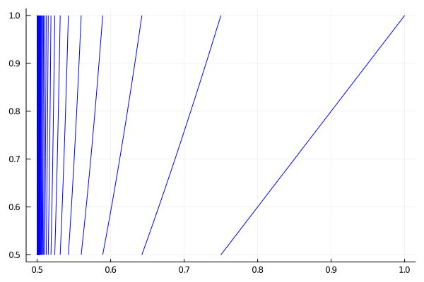
Figure 1. The inducing scheme for TT in (7.1).

We construct the inducing scheme as in Subsection 2.1. Let x0′=1x^{\prime}_{0}=1, x1′=34x^{\prime}_{1}=\frac{3}{4}, and

xn′=gω​(12)​for​n≥2.x^{\prime}_{n}=g_{\omega}(\frac{1}{2})\,\,\text{for}\,\,n\geq 2.

Letting ω=10n\omega=10^{n} and gω=g1∘g0ng_{\omega}=g_{1}\circ g_{0}^{n}, then cylinder set [ω][\omega] is given by gω​([0.5,1])=(xn′,xn−1′]g_{\omega}([0.5,1])=(x^{\prime}_{n},x^{\prime}_{n-1}].

Then T^:Δ→Δ\hat{T}:\Delta\to\Delta is a piecewise smooth and onto map with countable number of branches and it satisfies all the assumptions of subsection 2.1. See Figure 1 for a pictorial representation of the above inducing scheme.

7.1.1. Numerical remark: the Shooting Method

To approximate rigorously the operators in this paper we need a rigorous way to approximate long orbits given a coding, i.e., we need to be able to compute

x=gω​(y)=g1∘g0n−1​(y)x=g_{\omega}(y)=g_{1}\circ g_{0}^{n-1}(y)

i.e. we need to be able to compute x∈[0.5,1]x\in[0.5,1] such that

Tn+1​(x)=y,Ti​(x)∈[0,0.5]T^{n+1}(x)=y,\quad T^{i}(x)\in[0,0.5]

for i∈{1,…,n}i\in\{1,\dots,n\}.

To solve this problem efficiently and obtain tight bounds on xx is tricky taking preimages sequentially leads to propagation of errors and the computed interval ends up being not usable.

The main idea is to substitute the equation above with the following system of equations (this tecnique is called the Shooting Method, and we were introduced to it by W. Tucker)

{T⁡(x1)−x2=0x1∈[0.5,1]T⁡(x2)−x3=0x2∈[0,0.5]T⁡(x3)−x4=0x3∈[0,0.5]⋮T⁡(xn)−y=0xn∈[0,0.5].\left\{\begin{array}[]{cc}T(x_{1})-x_{2}=0&x_{1}\in[0.5,1]\\ T(x_{2})-x_{3}=0&x_{2}\in[0,0.5]\\ T(x_{3})-x_{4}=0&x_{3}\in[0,0.5]\\ \vdots&\\ T(x_{n})-y=0&x_{n}\in[0,0.5].\end{array}\right.

We will use the rigorous Newton method [42], to simultaneously enclose x1,…,xnx_{1},\ldots,x_{n}. This way we are solving a unique system of equations instead of propagating backwards the error through solving equations with a “fat” variable. Given a function ϕ:ℝn→ℝn\phi:\mathbb{R}^{n}\to\mathbb{R}^{n} and a vector of intervals x^=(x^1,…,x^n)\hat{x}=(\hat{x}_{1},\ldots,\hat{x}_{n}) the rigorous Newton step is given by

N⁡(x^)=x^∩mid​(x^)−D​ϕ​(x^)−1​ϕ​(mid​(x^)),N(\hat{x})=\hat{x}\cap\textrm{mid}(\hat{x})-D\phi(\hat{x})^{-1}\phi(\textrm{mid}(\hat{x})),

where the intersection between interval vectors is meant componentwise and mid is a function that sends a vector of intervals to the vector of their midpoints [42].

In our specific case, the shooting method is numerically well behaved: denoting by ϕ⁡(x1,…,xn)=(T⁡(x1)−x2,…,T⁡(xn)−y)T\phi(x_{1},\ldots,x_{n})=(T(x_{1})-x_{2},\ldots,T(x_{n})-y)^{T}, the Jacobian D​ϕD\phi is given by a bidiagonal matrix, whose i−t​hi-th diagonal entry is T′​(xi)T^{\prime}(x_{i}) and the superdiagonal entries are constant and equal to −1-1. In particular, this guarantees us that the Jacobian is invertible, since its eigenvalues correspond to the diagonal elements and these are bounded away from 00. Moreover a bidiagonal system is solved in time O⁡(n)O(n) by backsubstitution, with small numerical error, and these assumptions guarantee that the interval Newton method converges.

This allows us to compute tight enclosure of gω​(y)g_{\omega}(y), gω′​(y)g^{\prime}_{\omega}(y), which allows us to compute discretizations of the transfer operator.

7.2. Computing the error when taking a finite number of branches

Since we cannot calculate values for maps with infinitely many branches on the computer we use an approximating map as described in subsection 3.1,

Refer to caption
Figure 2. The approximation map with k=k=200

this is depicted in figure 2 for α=\alpha=0.125. To calculate bounds on the C1C^{1} distance between the systems these maps define we use lemma 3.1 and find DD and D0D_{0} for LSV maps. Estimating these bounds efficiently is delicate since it involves estimating the sum (and the tail) of converging series whose general term is going to zero slowly. The estimates in literature [5, 32] give rise to values that are impractical for our computations; as an example, the value of the constant C8C_{8} in [32] computed according to their proof is of the order of 1026910^{269}, which makes its use in our computations unfeasible, therefore some work is needed to give sharper bounds for the constants. Since these estimates are quite technical and need the introduction of specific notations, we separate them in the appendix not to hinder the flow of the sections.

In section 8.2 we bound D0≤D_{0}\leq0.2513 and D≤D\leq1.286, so

‖(L^−L^δk)‖C1≤(D+D0D+2)δk≤ 3.609 δk\left\lVert(\hat{L}-\hat{L}_{\delta_{k}})\right\rVert_{C^{1}}\leq(D+D_{0}D+2)\delta_{k}\leq\text{ $3.609$ }\delta_{k}

can be made as small as needed by increasing kk.

Choosing k=k=200 gives ‖L^−L^δk‖C1≤\left\lVert\hat{L}-\hat{L}_{\delta_{k}}\right\rVert_{C^{1}}\leq 7.743⋅10−127.743\cdot 10^{-12} .

7.2.1. Bounding ‖h^δk−h^‖C1\left\lVert\hat{h}_{\delta_{k}}-\hat{h}\right\rVert_{C^{1}}

In section 8.2.1 we prove the following Lasota-Yorke inequality

‖L^δkn​f‖C1≤2.491⋅(0.5)n​‖f‖C1+6.206​‖f‖∞\left\lVert\hat{L}^{n}_{\delta_{k}}f\right\rVert_{C^{1}}\leq\text{$$2.491$$}\cdot(0.5)^{n}\left\lVert f\right\rVert_{C^{1}}+\text{$$6.206$$}\left\lVert f\right\rVert_{\infty}

.

The Lasota-Yorke inequality implies that

‖L^δkn​f‖C1≤7.452,\left\lVert\hat{L}^{n}_{\delta_{k}}f\right\rVert_{C^{1}}\leq\textrm{$$7.452$$},

which together with Lemma 3.3, and the fact proved in section 7.3.1 by using the methods from [21] that

‖L^δk4|U0‖C1≤0.1557\left\lVert\hat{L}_{\delta_{k}}^{\text{$$4$$}}|_{U^{0}}\right\rVert_{C^{1}}\leq\text{$$0.1557$$}

allowing us to bound

(7.2) ‖h^−h^δk‖C1≤ 4 ⋅ 7.452 1− 0.1557 ‖(L^δk−L^)h^‖C1≤ 2.734⋅10−10 ‖h^‖C1\left\lVert\hat{h}-\hat{h}_{\delta_{k}}\right\rVert_{C^{1}}\leq\frac{\text{ $4$ }\cdot\text{ $7.452$ }}{1-\text{ $0.1557$ }}\left\lVert(\hat{L}_{\delta_{k}}-\hat{L})\hat{h}\right\rVert_{C^{1}}\leq\text{ $2.734\cdot 10^{-10}$ }\left\lVert\hat{h}\right\rVert_{C^{1}}

Observing that ‖h^‖C1≤‖h^δk‖C1+‖h^−h^δk‖C1\left\lVert\hat{h}\right\rVert_{C^{1}}\leq\left\lVert\hat{h}_{\delta_{k}}\right\rVert_{C^{1}}+\left\lVert\hat{h}-\hat{h}_{\delta_{k}}\right\rVert_{C^{1}} and a bound on ‖h^δk‖C1\left\lVert\hat{h}_{\delta_{k}}\right\rVert_{C^{1}} in section 8.2.1 gives us a final error of 2.113⋅10−92.113\cdot 10^{-9} .

7.2.2. Computing the discretization error

The truncated operator L^δk\hat{L}_{\delta_{k}} satisfies the following Lasota-Yorke like inequalities88 8 it is straightforward to see that these inequalities imply Lasota-Yorke inequalities on Wk,1W^{k,1} with weak norm Wk−1,1W^{k-1,1}.

‖(L^δkn)​f′‖1≤\displaystyle||(\hat{L}_{\delta_{k}}^{n})f^{\prime}||_{1}\leq λn​‖f′‖1+1.785​‖f‖1\displaystyle\lambda^{n}||f^{\prime}||_{1}+1.785||f||_{1}
‖(L^δkn)​f′′‖1≤\displaystyle||(\hat{L}_{\delta_{k}}^{n})f^{\prime\prime}||_{1}\leq λn​‖f′′‖1+0.3076​‖f′‖1+6.57||f||1\displaystyle\lambda^{n}||f^{\prime\prime}||_{1}+0.3076||f^{\prime}||_{1}+6.57||f||_{1}
‖(L^δk​f)′′′‖1≤\displaystyle||(\hat{L}_{\delta_{k}}f)^{\prime\prime\prime}||_{1}\leq λ3​n​‖f′′′‖1+0.145​‖f′′‖1+1.98​‖f′‖1+36.96||f||1\displaystyle\lambda^{3n}||f^{\prime\prime\prime}||_{1}+0.145||f^{\prime\prime}||_{1}+1.98||f^{\prime}||_{1}+36.96||f||_{1}
‖(L^δkn​f)(4)‖1≤\displaystyle||(\hat{L}_{\delta_{k}}^{n}f)^{(4)}||_{1}\leq λ4​n​‖f(4)‖1+0.057​‖f(3)‖1+1.49​||f′′||1+16.97|​|f′||1+559.4||f||1\displaystyle\lambda^{4n}||f^{(4)}||_{1}+0.057||f^{(3)}||_{1}+1.49||f^{\prime\prime}||_{1}+16.97||f^{\prime}||_{1}+559.4||f||_{1}
‖(L^δkn​f)(5)‖1≤\displaystyle||(\hat{L}_{\delta_{k}}^{n}f)^{(5)}||_{1}\leq λ5​n​‖f(5)‖1+0.0199​‖f(4)‖1+0.85||f(3)||1\displaystyle\lambda^{5n}||f^{(5)}||_{1}+0.0199||f^{(4)}||_{1}+0.85||f^{(3)}||_{1}
+\displaystyle+ 17.57​‖f′′‖1+794.59​‖f′‖1+10086||f||1\displaystyle 17.57||f^{\prime\prime}||_{1}+794.59||f^{\prime}||_{1}+10086||f||_{1}
‖(L^δkn​f)(6)‖1≤\displaystyle||(\hat{L}_{\delta_{k}}^{n}f)^{(6)}||_{1}\leq λ6​n​‖f(6)‖1+0.0066​‖f(5)‖1+0.41||f(4)||1\displaystyle\lambda^{6n}||f^{(6)}||_{1}+0.0066||f^{(5)}||_{1}+0.41||f^{(4)}||_{1}
+\displaystyle+ 13.33​‖f(3)‖1+895​‖f′′‖1+24840.2​‖f′‖1+684431||f||1.\displaystyle 13.33||f^{(3)}||_{1}+895||f^{\prime\prime}||_{1}+24840.2||f^{\prime}||_{1}+684431||f||_{1}.

Since we know ‖hδk‖1=1\left\lVert h_{\delta_{k}}\right\rVert_{1}=1 for ff a probability density, we can use these to get a bound on ‖hδk(6)‖1\left\lVert h_{\delta_{k}}^{(6)}\right\rVert_{1} which is calculated to be 7.953⋅1057.953\cdot 10^{5} . Denoting by L^n=πn​L^δk​πn\hat{L}_{n}=\pi_{n}\hat{L}_{\delta_{k}}\pi_{n} the discretized operator on the base of Chebyshev polynomials of the first kind of degree up to nn, the same Lasota-Yorke inequalities allow us to compute

‖L^δk−L^n‖C1≤ 3.297⋅10−11 .\left\lVert\hat{L}_{\delta_{k}}-\hat{L}_{n}\right\rVert_{C^{1}}\leq\text{ $3.297\cdot 10^{-11}$ }.

This, together with the computed bounds on the C1C^{1} mixing rate in table 1

Table 1. Calculated contraction rates of our discretised operators.
k ‖L^nk|U0‖C1\left\lVert\hat{L}_{n}^{k}|_{U^{0}}\right\rVert_{C^{1}}
1 3.6743.674
2 1.2541.254
3 0.42370.4237
4 0.14270.1427
5 0.047990.04799
6 0.016130.01613
7 0.0054210.005421
8 0.0018210.001821
9 0.00061190.0006119
10 0.00020560.0002056
11 0.00075510.0007551

gives us an error of

‖h^−h^n‖C1≤ 3.833⋅10−9 ;\left\lVert\hat{h}-\hat{h}_{n}\right\rVert_{C^{1}}\leq\text{ $3.833\cdot 10^{-9}$ };

in figure 3 a plot of the approximated density is presented.

Refer to caption
Figure 3. The invariant density of the induced map as calculated according to section 3.1.

7.2.3. Numerical remark: automated Lasota-Yorke inequalities

We detail a way to automatically calculate Lasota-Yorke type inequalities for transfer operators in Wk,1W^{k,1}. Following [11] let

Lk​f=∑y∈T−1​(x)f⁡(y)|T′​(y)|k.L_{k}f=\sum_{y\in T^{-1}(x)}\frac{f(y)}{|T^{\prime}(y)|^{k}}.

From this follows

(7.3) (Lk​f)′=Lk+1​f′+k​Lk​(f​D),(L_{k}f)^{\prime}=L_{k+1}f^{\prime}+kL_{k}(fD),

where D=(1/T′​(x))′D=(1/T^{\prime}(x))^{\prime} is the distorsion. We use the formula above to compute symbolical expressions for the derivatives (L1​f)(l)(L_{1}f)^{(l)}.

We use Interval Arithmetic and higher order Automatic Differentiation [42](as implemented in TaylorSeries.jl) to compute bounds for

‖(1/T′)(l)‖∞.\left\lVert(1/T^{\prime})^{(l)}\right\rVert_{\infty}.

This allows us to bound the coefficients of the Lasota-Yorke inequalities.

7.3. Approximating the linear response for the induced map

Refer to caption
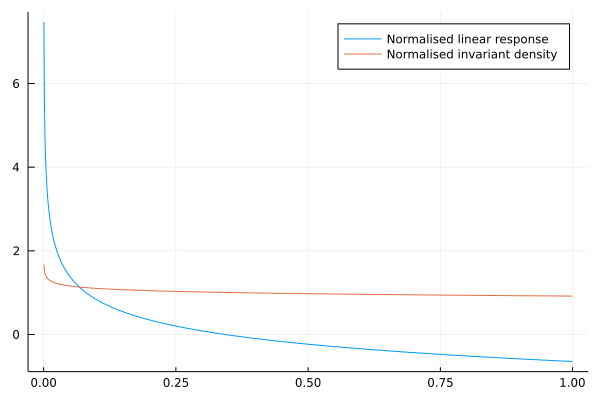
Figure 4. The linear response of the induced map as calculated according to Section 4.

We approximate the linear response of our induced map using (4.1) which uses the discretized operator P^h\hat{P}_{h}, associated to the hat discretization of size η=\eta= 9.537⋅10−79.537\cdot 10^{-7} . We get our error from lemma 4.6, which gives us four terms that need to be bound, each of which is done in the appendix, 7.3.3, 7.3.4, 7.3.5 and 7.3.7 for l∗=l^{*}= 988988 and k=k= 200200 :††margin: Toby▶\blacktriangleright Some changes here

  1. (1)

    ∑n=0l∗∑i=0n‖L^i|U0‖C0​‖(L^w−L^δk)​L^wn−i​Wh‖C0≤\sum_{n=0}^{l^{*}}\sum_{i=0}^{n}\left\lVert\hat{L}^{i}|_{U^{0}}\right\rVert_{C^{0}}\left\lVert(\hat{L}_{w}-\hat{L}_{\delta_{k}})\hat{L}_{w}^{n-i}W_{h}\right\rVert_{C^{0}}\leq 0.00076620.0007662

  2. (2)

    ∑n=1l∗∑i=0n−1‖L^i|U0‖C0​‖(L^δk−L^)​L^wn−i​Wh‖C0≤\sum_{n=1}^{l^{*}}\sum_{i=0}^{n-1}\left\lVert\hat{L}^{i}|_{U^{0}}\right\rVert_{C^{0}}\left\lVert(\hat{L}_{\delta_{k}}-\hat{L})\hat{L}_{w}^{n-i}W_{h}\right\rVert_{C^{0}}\leq 9.616⋅10−89.616\cdot 10^{-8}

  3. (3)

    ∑n=0l∗‖L^n|U0‖C0​‖Wh−W‖C0≤\sum_{n=0}^{l^{*}}\left\lVert\hat{L}^{n}|_{U^{0}}\right\rVert_{C^{0}}\left\lVert W_{h}-W\right\rVert_{C^{0}}\leq 3.055⋅10−73.055\cdot 10^{-7}

  4. (4)

    ∑n=l∗+1∞‖L^n​W‖C0≤\sum_{n=l^{*}+1}^{\infty}\left\lVert\hat{L}^{n}W\right\rVert_{C^{0}}\leq 2⋅10−2892\cdot 10^{-289}

this gives us a total error ‖h^∗−h^η∗‖C0≤\left\lVert\hat{h}^{*}-\hat{h}_{\eta}^{*}\right\rVert_{C^{0}}\leq 0.00076660.0007666

7.3.1. The contraction rates of L^δk\hat{L}_{\delta_{k}} in the C0C^{0} norm.

In order to bound ‖L^δkn|U0‖C0\left\lVert\hat{L}^{n}_{\delta_{k}}|_{U^{0}}\right\rVert_{C^{0}} we use lemma 7.13 from [4] to bound

‖(L^δkm−L^nm)​f‖C0≤Am​‖f‖C1+Bm​‖f‖C0\left\lVert(\hat{L}_{\delta_{k}}^{m}-\hat{L}_{n}^{m})f\right\rVert_{C^{0}}\leq A_{m}\left\lVert f\right\rVert_{C^{1}}+B_{m}\left\lVert f\right\rVert_{C^{0}}

from which we can use Cc,mC_{c,m} to bound ‖L^δkm|U0‖C0≤A​‖f‖C1+(B+Cc,m)​‖f‖C0\left\lVert\hat{L}_{\delta_{k}}^{m}|_{U^{0}}\right\rVert_{C^{0}}\leq A\left\lVert f\right\rVert_{C^{1}}+(B+C_{c,m})\left\lVert f\right\rVert_{C^{0}} and the Lasota-Yorke inequality (3) from section 8.2.1, and use the small matrix method from [20]. We have

(‖L^δkm​f‖C1‖L^δkm​f‖C0)≤(M​λmDAnBn+Cc,m)​(‖f‖C1‖f‖C0).\begin{pmatrix}\left\lVert\hat{L}^{m}_{\delta_{k}}f\right\rVert_{C^{1}}\\ \left\lVert\hat{L}^{m}_{\delta_{k}}f\right\rVert_{C^{0}}\end{pmatrix}\leq\begin{pmatrix}M\lambda^{m}&D\\ A_{n}&B_{n}+C_{c,m}\end{pmatrix}\begin{pmatrix}\left\lVert f\right\rVert_{C^{1}}\\ \left\lVert f\right\rVert_{C^{0}}\end{pmatrix}.

Choosing the value of nn that minimises equation (7.2), we take Cc,4≤C_{c,4}\leq 0.14270.1427 from section 7.2.2, together with the calculation ‖(L^δk4−L^n4)​f‖C0≤\left\lVert(\hat{L}_{\delta_{k}}^{4}-\hat{L}_{n}^{4})f\right\rVert_{C^{0}}\leq 8.5⋅10−78.5\cdot 10^{-7} ‖f‖C1+\left\lVert f\right\rVert_{C^{1}}+ 3.203⋅10−63.203\cdot 10^{-6} ‖f‖C0\left\lVert f\right\rVert_{C^{0}}, which gives the largest eigenvalue of the small matrix ρ=\rho= 0.15570.1557 .

7.3.2. The contraction rates of L^\hat{L} in the C0C^{0} norm.

We can use ‖L^δkn|U0‖C0≤ρn,C0\left\lVert\hat{L}_{\delta_{k}}^{n}|_{U^{0}}\right\rVert_{C^{0}}\leq\rho_{n,C^{0}} and parts of lemma 3.1 to get

‖L^n|U0‖C0≤‖L^δkn|U0‖C0+‖L^δkn−L^n‖C0≤n​C∗​(2+D)​δk+ρn,C0.\left\lVert\hat{L}^{n}|_{U^{0}}\right\rVert_{C^{0}}\leq\left\lVert\hat{L}_{\delta_{k}}^{n}|_{U^{0}}\right\rVert_{C^{0}}+\left\lVert\hat{L}^{n}_{\delta_{k}}-\hat{L}^{n}\right\rVert_{C^{0}}\leq nC^{*}(2+D)\delta_{k}+\rho_{n,C^{0}}.

These give us ‖L^n|U0‖C0≤\left\lVert\hat{L}^{n}|_{U^{0}}\right\rVert_{C^{0}}\leq 2.991⋅10−72.991\cdot 10^{-7} for n=n= 2222 .

7.3.3. Bounding Item (1)

We can bound ∑n=0l∗∑i=0n‖L^i|U0‖C0​‖(P^h−L^δk)​P^hn−i​Wh‖C0\sum_{n=0}^{l^{*}}\sum_{i=0}^{n}\left\lVert\hat{L}^{i}|_{U^{0}}\right\rVert_{C^{0}}\left\lVert(\hat{P}_{h}-\hat{L}_{\delta_{k}})\hat{P}_{h}^{n-i}W_{h}\right\rVert_{C^{0}} by

∑n=0l∗∑i=0n‖L^i​(P^h−L^δk)​P^hn−i​Wh‖C0\displaystyle\sum_{n=0}^{l^{*}}\sum_{i=0}^{n}\left\lVert\hat{L}^{i}(\hat{P}_{h}-\hat{L}_{\delta_{k}})\hat{P}_{h}^{n-i}W_{h}\right\rVert_{C^{0}}
≤\displaystyle\leq η​K​∑n=0l∗∑i=0n‖L^i|U0‖C0​(Lip​(P^hn−i​Wh)+‖P^hn−i​Wh‖C0)\displaystyle\eta K\sum_{n=0}^{l^{*}}\sum_{i=0}^{n}\left\lVert\hat{L}^{i}|_{U^{0}}\right\rVert_{C^{0}}(\textrm{Lip}(\hat{P}_{h}^{n-i}W_{h})+\left\lVert\hat{P}_{h}^{n-i}W_{h}\right\rVert_{C^{0}})

where K=2​(D+1+λ⁡(D+1))K=2(D+1+\lambda(D+1)).

We can calculate Lip​(P^hn−i​Wh)\textrm{Lip}{(\hat{P}_{h}^{n-i}W_{h}}) and ‖P^hn−i​Wh‖C0\left\lVert\hat{P}_{h}^{n-i}W_{h}\right\rVert_{C^{0}} explictly by using validated numerical methods, since WhW_{h} explicitly represented on the computer, so we can compute an enclosure of P^h​Wh\hat{P}_{h}W_{h} by rigorous matrix multiplication; for a function ff in the hat basis with coefficients viv_{i} we have explicit functions that allow us to compute the Lip and C0C^{0} norm, i.e.:

Lip​(f)=max⁡|vi+1−vi|η,‖f‖C0=maxi⁡|vi|.\quad\textrm{Lip}(f)=\max\frac{|v_{i+1}-v_{i}|}{\eta},\quad||f||_{C^{0}}=\max_{i}|v_{i}|.

We calculate this to give

∑n=0l∗∑i=0n‖L^i(P^h−L^δk)P^hn−iWh‖C0≤ 0.0007662 \sum_{n=0}^{l^{*}}\sum_{i=0}^{n}\left\lVert\hat{L}^{i}(\hat{P}_{h}-\hat{L}_{\delta_{k}})\hat{P}_{h}^{n-i}W_{h}\right\rVert_{C^{0}}\leq\text{ $0.0007662$ }

7.3.4. Bounding Item (2)

To bound ∑n=1l∗∑i=0n−1‖L^i​(L^δk−L^)​P^hn−i​Wh‖C0\sum_{n=1}^{l^{*}}\sum_{i=0}^{n-1}\left\lVert\hat{L}^{i}(\hat{L}_{\delta_{k}}-\hat{L})\hat{P}_{h}^{n-i}W_{h}\right\rVert_{C^{0}}, observe

∑n=0l∗∑i=0n‖L^i​(L^δk−L^)​P^hn−i​Wh‖C0\displaystyle\sum_{n=0}^{l^{*}}\sum_{i=0}^{n}\left\lVert\hat{L}^{i}(\hat{L}_{\delta_{k}}-\hat{L})\hat{P}_{h}^{n-i}W_{h}\right\rVert_{C^{0}}
≤\displaystyle\leq ∑n=0l∗∑i=0n‖L^i‖C0​‖(L^δk−L^)​P^hn−i​Wh‖C0\displaystyle\sum_{n=0}^{l^{*}}\sum_{i=0}^{n}\left\lVert\hat{L}^{i}\right\rVert_{C^{0}}\left\lVert(\hat{L}_{\delta_{k}}-\hat{L})\hat{P}_{h}^{n-i}W_{h}\right\rVert_{C^{0}}

and

‖(L^δk−L^)​f‖C0\displaystyle\left\lVert(\hat{L}_{\delta_{k}}-\hat{L})f\right\rVert_{C^{0}}
≤\displaystyle\leq ‖f⁡(δk​(2​x−1)+12)​2​δk−∑|ω|>N∗f∘gω​|gω′|‖C0\displaystyle\left\lVert f(\delta_{k}(2x-1)+\frac{1}{2})2\delta_{k}-\sum_{|\omega|>N^{*}}f\circ g_{\omega}|g_{\omega}^{\prime}|\right\rVert_{C^{0}}
≤\displaystyle\leq 2​δk​‖f⁡(δk​(2​x−1)+12)‖C0+∑|ω|>N∗‖f∘gω​|gω′|‖C0\displaystyle 2\delta_{k}\left\lVert f(\delta_{k}(2x-1)+\frac{1}{2})\right\rVert_{C^{0}}+\sum_{|\omega|>N^{*}}\left\lVert f\circ g_{\omega}|g_{\omega}^{\prime}|\right\rVert_{C^{0}}
≤\displaystyle\leq (2​δk+∑|ω|>N∗|gω′|)​‖f‖C0\displaystyle(2\delta_{k}+\sum_{|\omega|>N^{*}}|g_{\omega}^{\prime}|)\left\lVert f\right\rVert_{C^{0}}

and therefore we have an upper bound of

(2​δk+∑|ω|>N∗|gω′|)​∑n=0l∗∑i=0n‖L^i‖C0​‖P^hn−i​Wh‖C0(2\delta_{k}+\sum_{|\omega|>N^{*}}|g_{\omega}^{\prime}|)\sum_{n=0}^{l^{*}}\sum_{i=0}^{n}\left\lVert\hat{L}^{i}\right\rVert_{C^{0}}\left\lVert\hat{P}_{h}^{n-i}W_{h}\right\rVert_{C^{0}}

As in the estimate for item (1) we can compute ‖P^hn−i​Wh‖C0\left\lVert\hat{P}_{h}^{n-i}W_{h}\right\rVert_{C^{0}} explicitly, which gives us

∑n=1l∗∑i=0n−1‖L^i(L^δk−L^)P^hn−iWh‖C0≤ 9.616⋅10−8 .\sum_{n=1}^{l^{*}}\sum_{i=0}^{n-1}\left\lVert\hat{L}^{i}(\hat{L}_{\delta_{k}}-\hat{L})\hat{P}_{h}^{n-i}W_{h}\right\rVert_{C^{0}}\leq\text{ $9.616\cdot 10^{-8}$ }.

7.3.5. Bounding Item (3)

We bound ‖Wh−W‖C0\left\lVert W_{h}-W\right\rVert_{C^{0}} by the following

‖Wh−W‖C0≤‖Wh−W∞‖C0+2​Lip​(W)​η,\left\lVert W_{h}-W\right\rVert_{C^{0}}\leq\left\lVert W_{h}-W_{\infty}\right\rVert_{C^{0}}+2\textrm{Lip}(W)\eta,

as explained in remark 4.4.

Remark that Lip​(W)=‖W′‖∞\textrm{Lip}(W)=\left\lVert W^{\prime}\right\rVert_{\infty} that we computed in section 7.3.6 to be bounded by 1.08287⋅10−51.08287\cdot 10^{-5} .

Recall that

Wh=∑i=0hai​ϕi​(x)W_{h}=\sum_{i=0}^{h}a_{i}\phi_{i}(x)

and

W∞=∑i=0ha~i​ϕi​(x)W_{\infty}=\sum_{i=0}^{h}\tilde{a}_{i}\phi_{i}(x)

where

ai=∑ω≤k1η​∫gω​(Ii)A0​(z)⋅h^n′​(ζ)+B0​(z)​h^n​(ζ)​𝑑z+1η​∫δk​(2​Ii−1)+1/2[A0​h^η′+B0​h^n]​(z)​𝑑za_{i}=\sum_{\omega\leq k}\frac{1}{\eta}\int_{g_{\omega}(I_{i})}A_{0}(z)\cdot\hat{h}_{n}^{\prime}(\zeta)+B_{0}(z)\hat{h}_{n}(\zeta)dz+\frac{1}{\eta}\int_{\delta_{k}(2I_{i}-1)+1/2}[A_{0}\hat{h}^{\prime}_{\eta}+B_{0}\hat{h}_{n}](z)dz

and

a~i=∫IiL^​(A0​h′+B0​h)=∑ω1η​∫gω​(Ii)A0​(x)⋅h^′​(x)+B0​(x)​h^​(x)​𝑑x\tilde{a}_{i}=\int_{I_{i}}\hat{L}(A_{0}h^{\prime}+B_{0}h)=\sum_{\omega}\frac{1}{\eta}\int_{g_{\omega}(I_{i})}A_{0}(x)\cdot\hat{h}^{\prime}(x)+B_{0}(x)\hat{h}(x)dx

Then we have that

‖Wh−W∞‖C0≤sup|ai−a~i|.||W_{h}-W_{\infty}||_{C^{0}}\leq\sup|a_{i}-\tilde{a}_{i}|.

We introduce auxiliary quantities

ai,∗=∑ω1η​∫gω​(Ii)A0​(x)⋅h^′​(ζ)+B0​(x)​h^​(ζ)​𝑑xa_{i,*}=\sum_{\omega}\frac{1}{\eta}\int_{g_{\omega}(I_{i})}A_{0}(x)\cdot\hat{h}^{\prime}(\zeta)+B_{0}(x)\hat{h}(\zeta)dx

where the ζ\zeta in gω​(Ii)g_{\omega}(I_{i}) is chosen as in the computation of aia_{i} for all ii and for all ω<k\omega<k, and arbitrarily for all ω≥k\omega\geq k.

Then

|a~i−ai,∗|=|∑ω1η​∫gω​(Ii)A0​(x)⋅h^′​(x)+B0​(x)​h^​(x)​𝑑x−∫gω​(Ii)A0​(x)⋅h^n′​(ζ)+B0​(x)​h^n​(ζ)​𝑑x|\displaystyle|\tilde{a}_{i}-a_{i,*}|=\left|\sum_{\omega}\frac{1}{\eta}\int_{g_{\omega}(I_{i})}A_{0}(x)\cdot\hat{h}^{\prime}(x)+B_{0}(x)\hat{h}(x)dx-\int_{g_{\omega}(I_{i})}A_{0}(x)\cdot\hat{h}_{n}^{\prime}(\zeta)+B_{0}(x)\hat{h}_{n}(\zeta)dx\right|
=\displaystyle= |∑ω1η​∫gω​(Ii)A0​(x)⋅(h^′​(x)−h^n′​(ζ))+B0​(x)​(h^​(x)−h^n​(ζ))​𝑑x|\displaystyle\left|\sum_{\omega}\frac{1}{\eta}\int_{g_{\omega}(I_{i})}A_{0}(x)\cdot(\hat{h}^{\prime}(x)-\hat{h}^{\prime}_{n}(\zeta))+B_{0}(x)(\hat{h}(x)-\hat{h}_{n}(\zeta))dx\right|
≤\displaystyle\leq ∑ω(|gω​(Ii)|​‖h^′′‖∞+‖h^′−h^n′‖∞)​1η​|∫gω​(Ii)A0​(x)​𝑑x|\displaystyle\sum_{\omega}(|g_{\omega}(I_{i})|\left\lVert\hat{h}^{\prime\prime}\right\rVert_{\infty}+\left\lVert\hat{h}^{\prime}-\hat{h}_{n}^{\prime}\right\rVert_{\infty})\frac{1}{\eta}\left|\int_{g_{\omega}(I_{i})}A_{0}(x)dx\right|
+(|gω​(Ii)|​‖h^′‖∞+‖h^−h^n‖∞)​1η​|∫gω​(Ii)B0​(x)​𝑑x|.\displaystyle+(|g_{\omega}(I_{i})|\left\lVert\hat{h}^{\prime}\right\rVert_{\infty}+\left\lVert\hat{h}-\hat{h}_{n}\right\rVert_{\infty})\frac{1}{\eta}\left|\int_{g_{\omega}(I_{i})}B_{0}(x)dx\right|.

Recalling that A0=∂ϵgω​(T^ϵ)A_{0}=\partial_{\epsilon}g_{\omega}(\hat{T}_{\epsilon}) B0=∂ϵgω′​(T^ϵ)⋅T^ϵ′B_{0}=\partial_{\epsilon}g_{\omega}^{\prime}(\hat{T}_{\epsilon})\cdot\hat{T}^{\prime}_{\epsilon} 99 9 Note that while this appears to depend on ω\omega, we choose the value of ω\omega coresponding to the appropriate branch of T^ϵ\hat{T}_{\epsilon}. we get

supi∑ω(|gω​(Ii)|​‖h^′′‖∞+‖h^′−h^n′‖∞)​1η​|∫gω​(Ii)A0​(x)​𝑑x|\displaystyle\sup_{i}\sum_{\omega}(|g_{\omega}(I_{i})|\left\lVert\hat{h}^{\prime\prime}\right\rVert_{\infty}+\left\lVert\hat{h}^{\prime}-\hat{h}_{n}^{\prime}\right\rVert_{\infty})\frac{1}{\eta}\left|\int_{g_{\omega}(I_{i})}A_{0}(x)dx\right|
+(|gω​(Ii)|​‖h^′‖∞+‖h^−h^n‖∞)​1η​|∫gω​(Ii)B0​(x)​𝑑x|\displaystyle+(|g_{\omega}(I_{i})|\left\lVert\hat{h}^{\prime}\right\rVert_{\infty}+\left\lVert\hat{h}-\hat{h}_{n}\right\rVert_{\infty})\frac{1}{\eta}\left|\int_{g_{\omega}(I_{i})}B_{0}(x)dx\right|
≤\displaystyle\leq supi∑ω(|gω​(Ii)|​‖h^′′‖∞+‖h^′−h^n′‖∞)​1η​|∫Ii∂ϵgω​(x)​T^ϵ′​(x)|\displaystyle\sup_{i}\sum_{\omega}(|g_{\omega}(I_{i})|\left\lVert\hat{h}^{\prime\prime}\right\rVert_{\infty}+\left\lVert\hat{h}^{\prime}-\hat{h}_{n}^{\prime}\right\rVert_{\infty})\frac{1}{\eta}\left|\int_{I_{i}}\partial_{\epsilon}g_{\omega}(x)\hat{T}_{\epsilon}^{\prime}(x)\right|
+(|gω​(Ii)|​‖h^′‖∞+‖h^−h^n‖∞)​1η​|∫Ii∂ϵgω′​(x)​𝑑x|\displaystyle+(|g_{\omega}(I_{i})|\left\lVert\hat{h}^{\prime}\right\rVert_{\infty}+\left\lVert\hat{h}-\hat{h}_{n}\right\rVert_{\infty})\frac{1}{\eta}\left|\int_{I_{i}}\partial_{\epsilon}g_{\omega}^{\prime}(x)dx\right|
≤\displaystyle\leq (|gω​(Ii)|​‖h^‖C2+‖h^−h^n‖C1)​∑ω|∂ϵgω​T^ϵ′|+|∂ϵgω′|\displaystyle(|g_{\omega}(I_{i})|\left\lVert\hat{h}\right\rVert_{C^{2}}+\left\lVert\hat{h}-\hat{h}_{n}\right\rVert_{C^{1}})\sum_{\omega}|\partial_{\epsilon}g_{\omega}\hat{T}_{\epsilon}^{\prime}|+|\partial_{\epsilon}g_{\omega}^{\prime}|

which we calculate using methods from sections 7.3.6 and 9 for η=\eta= 9.537⋅10−79.537\cdot 10^{-7} to get

|a~i−ai,∗|≤ 3.046⋅10−7 .|\tilde{a}_{i}-a_{i,*}|\leq\text{ $3.046\cdot 10^{-7}$ }.

Now, denote by bb the linear branch of the truncated induced LSV map; then

|ai−ai,∗|=|1η​∫b−1​(Ii)A0​(y)​hn′​(ζ)+B0​(y)​h^n​(ζ)​𝑑y−1η​∑|ω|>k∫gω​(Ii)A0​(y)​hn′​(ζ)+B0​(y)​h^n​(ζ)​𝑑y||a_{i}-a_{i,*}|=\left|\frac{1}{\eta}\int_{b^{-1}(I_{i})}A_{0}(y)h^{\prime}_{n}(\zeta)+B_{0}(y)\hat{h}_{n}(\zeta)dy-\frac{1}{\eta}\sum_{|\omega|>k}\int_{g_{\omega}(I_{i})}A_{0}(y)h^{\prime}_{n}(\zeta)+B_{0}(y)\hat{h}_{n}(\zeta)dy\right|

for all ii.

We will only compute a bound for the B0B_{0} terms, the A0A_{0} terms are similar.

|1η​∫b−1​(Ii)B0​(y)​h^n​(ζ)​𝑑y−1η​∑|ω|>k∫gω​(Ii)B0​(y)​h^n​(ζ)​𝑑y|\displaystyle\left|\frac{1}{\eta}\int_{b^{-1}(I_{i})}B_{0}(y)\hat{h}_{n}(\zeta)dy-\frac{1}{\eta}\sum_{|\omega|>k}\int_{g_{\omega}(I_{i})}B_{0}(y)\hat{h}_{n}(\zeta)dy\right|
≤\displaystyle\leq |1η​∫b−1​(Ii)B0​(y)​h^n​(ζ)​𝑑y|+|1η​∑|ω|>k∫gω​(Ii)B0​(y)​h^n​(ζ)​𝑑y|\displaystyle\left|\frac{1}{\eta}\int_{b^{-1}(I_{i})}B_{0}(y)\hat{h}_{n}(\zeta)dy\right|+\left|\frac{1}{\eta}\sum_{|\omega|>k}\int_{g_{\omega}(I_{i})}B_{0}(y)\hat{h}_{n}(\zeta)dy\right|
≤\displaystyle\leq ‖h^n‖C0​(|1η​∫b−1​(Ii)B0​(y)​𝑑y|+∑|ω|>k|∂ϵgω′|)\displaystyle\left\lVert\hat{h}_{n}\right\rVert_{C^{0}}\left(\left|\frac{1}{\eta}\int_{b^{-1}(I_{i})}B_{0}(y)dy\right|+\sum_{|\omega|>k}|\partial_{\epsilon}g_{\omega}^{\prime}|\right)
≤\displaystyle\leq ‖h^n‖C0​(|δk2​η​∫IiB0​(b−1​(y))​𝑑y|+∑|ω|>k|∂ϵgω′|)\displaystyle\left\lVert\hat{h}_{n}\right\rVert_{C^{0}}\left(\left|\frac{\delta_{k}}{2\eta}\int_{I_{i}}B_{0}(b^{-1}(y))dy\right|+\sum_{|\omega|>k}|\partial_{\epsilon}g_{\omega}^{\prime}|\right)
≤\displaystyle\leq ‖h^n‖C0​(δk2​η​‖B0‖1+∑|ω|>k|∂ϵgω′|)\displaystyle\left\lVert\hat{h}_{n}\right\rVert_{C^{0}}\left(\frac{\delta_{k}}{2\eta}\left\lVert B_{0}\right\rVert_{1}+\sum_{|\omega|>k}|\partial_{\epsilon}g_{\omega}^{\prime}|\right)

which including the A0A_{0} term in a similar fashion we get

‖h^n‖C1​(δk2​η​max⁡{‖A0‖1,‖B0‖1}+∑|ω|>k(|∂ϵgω′|+|∂ϵgω⋅gω′|)).\left\lVert\hat{h}_{n}\right\rVert_{C^{1}}\left(\frac{\delta_{k}}{2\eta}\max\{\left\lVert A_{0}\right\rVert_{1},\left\lVert B_{0}\right\rVert_{1}\}+\sum_{|\omega|>k}(|\partial_{\epsilon}g_{\omega}^{\prime}|+|\partial_{\epsilon}g_{\omega}\cdot g_{\omega}^{\prime}|)\right).

Taking k=k= 200200 this allows us to prove that ‖Wh−W‖C0≤\left\lVert W_{h}-W\right\rVert_{C^{0}}\leq 3.055⋅10−73.055\cdot 10^{-7} .

7.3.6. Bounding ‖W′‖C0\left\lVert W^{\prime}\right\rVert_{C^{0}}

For calculating ‖W′‖C0\left\lVert W^{\prime}\right\rVert_{C^{0}}, first we observe that for the B0B_{0} term

(L^​[(B0​h^)∘gω⋅gω′])′\displaystyle(\hat{L}[(B_{0}\hat{h})\circ g_{\omega}\cdot g_{\omega}^{\prime}])^{\prime} =∑([∂ϵgω′​(Tϵ)​Tϵ′​h^]∘gω⋅gω′)′\displaystyle=\sum([\partial_{\epsilon}g^{\prime}_{\omega}(T_{\epsilon})T_{\epsilon}^{\prime}\hat{h}]\circ g_{\omega}\cdot g_{\omega}^{\prime})^{\prime}
=∑(∂ϵgω′​(h^∘gω))′\displaystyle=\sum(\partial_{\epsilon}g^{\prime}_{\omega}(\hat{h}\circ g_{\omega}))^{\prime}
=∑∂ϵgω′′​(h^∘gω)+∂ϵgω′​h^′∘gω​gω′\displaystyle=\sum\partial_{\epsilon}g_{\omega}^{\prime\prime}(\hat{h}\circ g_{\omega})+\partial_{\epsilon}g_{\omega}^{\prime}\hat{h}^{\prime}\circ g_{\omega}g_{\omega}^{\prime}
≤‖h^‖C1​max⁡{∑∂ϵgω′′,∑∂ϵgω′​gω′}\displaystyle\leq\left\lVert\hat{h}\right\rVert_{C^{1}}\max\{\sum\partial_{\epsilon}g_{\omega}^{\prime\prime},\sum\partial_{\epsilon}g_{\omega}^{\prime}g_{\omega}^{\prime}\}

from [32] lemma 5.8 and 5.3 we have that

∑∂ϵgω′′≤C​∑r=1∞4​(1−log⁡(0.5))r(α+1)/α≤C​4​(1−log⁡(0.5))​ζ′′​(9)\sum\partial_{\epsilon}g_{\omega}^{\prime\prime}\leq C\sum_{r=1}^{\infty}\frac{4(1-\log(0.5))}{r^{(\alpha+1)/\alpha}}\leq C4(1-\log(0.5))\zeta^{\prime\prime}(9)

so it remains to find this CC.

From the proof of lemma 5.8 we have

∂ϵzr′′=\displaystyle\partial_{\epsilon}z_{r}^{\prime\prime}= [2​α+1+α⁡(α+1)​log⁡(2​zr+1)]​2α​zr+1α−1​(zr+1′)2\displaystyle[2\alpha+1+\alpha(\alpha+1)\log(2z_{r+1})]2^{\alpha}z_{r+1}^{\alpha-1}(z_{r+1}^{\prime})^{2}
+\displaystyle+ (α−1)​α​(α+1)​2α​zr+1α−2​(zr+1′)2​∂ϵzr+1+2​α​(α+1)​2α​zr+1α−1​zr+1′​∂ϵzr+1′\displaystyle(\alpha-1)\alpha(\alpha+1)2^{\alpha}z_{r+1}^{\alpha-2}(z_{r+1}^{\prime})^{2}\partial_{\epsilon}z_{r+1}+2\alpha(\alpha+1)2^{\alpha}z_{r+1}^{\alpha-1}z_{r+1}^{\prime}\partial_{\epsilon}z_{r+1}^{\prime}
+\displaystyle+ (1+(α+1)​log⁡(2​zr+1))​2α​zr+1α​zr+1′′+α⁡(α+1)​2α​zr+1α−1​zr+1′′​∂ϵzr+1\displaystyle(1+(\alpha+1)\log(2z_{r+1}))2^{\alpha}z_{r+1}^{\alpha}z_{r+1}^{\prime\prime}+\alpha(\alpha+1)2^{\alpha}z_{r+1}^{\alpha-1}z_{r+1}^{\prime\prime}\partial_{\epsilon}z_{r+1}
+\displaystyle+ (1+(α+1)​2α​zr+1α)​∂ϵzr+1′′\displaystyle(1+(\alpha+1)2^{\alpha}z_{r+1}^{\alpha})\partial_{\epsilon}z_{r+1}^{\prime\prime}

which we divide by zr′=[1+(α+1)​2α​zr+1α]​zr+1′z_{r}^{\prime}=[1+(\alpha+1)2^{\alpha}z_{r+1}^{\alpha}]z_{r+1}^{\prime} to get

|∂ϵzr′′zr′−∂ϵzr+1′′zr+1′|≤\displaystyle\left|\frac{\partial_{\epsilon}z_{r}^{\prime\prime}}{z_{r}^{\prime}}-\frac{\partial_{\epsilon}z_{r+1}^{\prime\prime}}{z_{r+1}^{\prime}}\right|\leq OPEN2​α+1+α⁡(α+1)​log⁡(2))α+1​|zr+1α−1​zr+1′|+α​|log⁡(zr+1)​zr+1α−1​zr+1′|\displaystyle\frac{2\alpha+1+\alpha(\alpha+1)\log(2))}{\alpha+1}\left|z_{r+1}^{\alpha-1}z_{r+1}^{\prime}\right|+\alpha\left|\log(z_{r+1})z_{r+1}^{\alpha-1}z_{r+1}^{\prime}\right|
+\displaystyle+ (α−1)​α​(α+1)​2α​|zr+1α−2​zr+1′​∂ϵzr+1|+2​α​(α+1)​2α​|zr+1α−1​∂ϵzr+1′|\displaystyle(\alpha-1)\alpha(\alpha+1)2^{\alpha}\left|z_{r+1}^{\alpha-2}z_{r+1}^{\prime}\partial_{\epsilon}z_{r+1}\right|+2\alpha(\alpha+1)2^{\alpha}|z_{r+1}^{\alpha-1}\partial_{\epsilon}z_{r+1}^{\prime}|
+\displaystyle+ OPEN(2+(α+1)​log⁡(2)))​2α1+(α+1)​2α​|zr+1′′zr+1′|+|log⁡(zr+1)​zr+1′′zr+1′|\displaystyle\frac{(2+(\alpha+1)\log(2)))2^{\alpha}}{1+(\alpha+1)2^{\alpha}}\left|\frac{z_{r+1}^{\prime\prime}}{z_{r+1}^{\prime}}\right|+\left|\frac{\log(z_{r+1})z_{r+1}^{\prime\prime}}{z_{r+1}^{\prime}}\right|
+\displaystyle+ α​|zr+1α−1​zr+1′′​∂ϵzr+1zr+1′|\displaystyle\alpha\left|\frac{z_{r+1}^{\alpha-1}z_{r+1}^{\prime\prime}\partial_{\epsilon}z_{r+1}}{z_{r+1}^{\prime}}\right|

so we must find bounds on |zr+1α−1​zr+1′|\left|z_{r+1}^{\alpha-1}z_{r+1}^{\prime}\right|, |log⁡(zr+1)​zr+1α−1​zr+1′|\left|\log(z_{r+1})z_{r+1}^{\alpha-1}z_{r+1}^{\prime}\right|, |zr+1α−2​zr+1′​∂ϵzr+1|\left|z_{r+1}^{\alpha-2}z_{r+1}^{\prime}\partial_{\epsilon}z_{r+1}\right|, |zr+1′′zr+1′|\left|\frac{z_{r+1}^{\prime\prime}}{z_{r+1}^{\prime}}\right|, |log⁡(zr+1)​zr+1′′zr+1′|\left|\frac{\log(z_{r+1})z_{r+1}^{\prime\prime}}{z_{r+1}^{\prime}}\right| and |zr+1α−1​zr+1′′​∂ϵzr+1zr+1′|\left|\frac{z_{r+1}^{\alpha-1}z_{r+1}^{\prime\prime}\partial_{\epsilon}z_{r+1}}{z_{r+1}^{\prime}}\right|. We do this by [32] lemmas 5.2, 5.3, 5.4, 5.6 and 5.7.

Lemma 5.2 gives

C11/α​z0(r+1)1/α≤zr+1≤C21/α(r+1)1/α.\frac{C_{1}^{1/\alpha}z_{0}}{(r+1)^{1/\alpha}}\leq z_{r+1}\leq\frac{C_{2}^{1/\alpha}}{(r+1)^{1/\alpha}}.

Lemma 5.3 gives

zr+1′≤C8(1+(r+1)z0αα2α)−(α+1)/α≤C8(α2α)−(α+1)/α(r+1)−(α+1)/αz0−(α+1).z_{r+1}^{\prime}\leq C_{8}(1+(r+1)z_{0}^{\alpha}\alpha 2^{\alpha})^{-(\alpha+1)/\alpha}\leq C_{8}(\alpha 2^{\alpha})^{-(\alpha+1)/\alpha}(r+1)^{-(\alpha+1)/\alpha}z_{0}^{-(\alpha+1)}.

Lemma 5.4 gives

|zr+1′′zr+1′|≤α(α+1)2αC2(α−1)/αC8(α2α)−(α+1)/αz0−2max⁡{r+1,1}\left|\frac{z_{r+1}^{\prime\prime}}{z_{r+1}^{\prime}}\right|\leq\alpha(\alpha+1)2^{\alpha}C_{2}^{(\alpha-1)/\alpha}C_{8}(\alpha 2^{\alpha})^{-(\alpha+1)/\alpha}\frac{z_{0}^{-2}}{\max\{r+1,1\}}

Lemma 5.6 gives

|∂ϵzr|≤2α​C21/αα⁡(α+1)​2α−1​l​o​g​g​(r​z0α)r1/α​(l​o​g​g​(r)−log⁡(z0)).|\partial_{\epsilon}z_{r}|\leq\frac{2^{\alpha}C_{2}^{1/\alpha}}{\alpha(\alpha+1)2^{\alpha-1}}\frac{logg(rz_{0}^{\alpha})}{r^{1/\alpha}}(logg(r)-\log(z_{0})).

Lemma 5.7 gives

|∂ϵzr+1′zr+1′|​((α+2)​2α+2​α+11−α​C21/α)​[l​o​g​g​(r​z0α)]2​(l​o​g​g​(r)−log⁡(z0))\left|\frac{\partial_{\epsilon}z_{r+1}^{\prime}}{z_{r+1}^{\prime}}\right|((\alpha+2)2^{\alpha}+2\frac{\alpha+1}{1-\alpha}C_{2}^{1/\alpha})[logg(rz_{0}^{\alpha})]^{2}(logg(r)-\log(z_{0}))

Combining these gives

|zr+1α−1​zr+1′|≤\displaystyle\left|z_{r+1}^{\alpha-1}z_{r+1}^{\prime}\right|\leq C2(α−1)/αC8(α2α)−(α+1)/α(r+1)−2z0−(α+1)\displaystyle C_{2}^{(\alpha-1)/\alpha}C_{8}(\alpha 2^{\alpha})^{-(\alpha+1)/\alpha}(r+1)^{-2}z_{0}^{-(\alpha+1)}
|log⁡(zr+1)​zr+1α−1​zr+1′|≤\displaystyle\left|\log(z_{r+1})z_{r+1}^{\alpha-1}z_{r+1}^{\prime}\right|\leq C3C2(α−1)/αC8(α2α)−(α+1)/α(r+1)−2z0−(α+1)(logg(r+1)−log(z0))\displaystyle C_{3}C_{2}^{(\alpha-1)/\alpha}C_{8}(\alpha 2^{\alpha})^{-(\alpha+1)/\alpha}(r+1)^{-2}z_{0}^{-(\alpha+1)}(logg(r+1)-\log(z_{0}))
|zr+1α−2​zr+1′​∂ϵzr+1|≤\displaystyle\left|z_{r+1}^{\alpha-2}z_{r+1}^{\prime}\partial_{\epsilon}z_{r+1}\right|\leq C2(α−1)/α​C8​(α​2α)(α+1)/αα⁡(α+1)​2α−1​(r+1)−2​z0−α−1​l​o​g​g​(r​z0α)​(l​o​g​g​(r)−log⁡(z0))\displaystyle\frac{C_{2}^{(\alpha-1)/\alpha}C_{8}(\alpha 2^{\alpha})^{(\alpha+1)/\alpha}}{\alpha(\alpha+1)2^{\alpha-1}}(r+1)^{-2}z_{0}^{-\alpha-1}logg(rz_{0}^{\alpha})(logg(r)-\log(z_{0}))
|zr+1′′zr+1′|≤\displaystyle\left|\frac{z_{r+1}^{\prime\prime}}{z_{r+1}^{\prime}}\right|\leq α(α+1)2αC2(α−1)/αC8(α2α)−(α+1)/αz0−2max⁡{r+1,1}\displaystyle\alpha(\alpha+1)2^{\alpha}C_{2}^{(\alpha-1)/\alpha}C_{8}(\alpha 2^{\alpha})^{-(\alpha+1)/\alpha}\frac{z_{0}^{-2}}{\max\{r+1,1\}}
|log⁡(zr+1)​zr+1′′zr+1′|≤\displaystyle\left|\frac{\log(z_{r+1})z_{r+1}^{\prime\prime}}{z_{r+1}^{\prime}}\right|\leq α(α+1)2αC2(α−1)/αC8(α2α)−(α+1)/αC3z0−2max⁡{r+1,1}(log(r+1)−log(z0))\displaystyle\alpha(\alpha+1)2^{\alpha}C_{2}^{(\alpha-1)/\alpha}C_{8}(\alpha 2^{\alpha})^{-(\alpha+1)/\alpha}C_{3}\frac{z_{0}^{-2}}{\max\{r+1,1\}}(\log(r+1)-\log(z_{0}))
|zr+1α−1​zr+1′′​∂ϵzr+1zr+1′|≤\displaystyle\left|\frac{z_{r+1}^{\alpha-1}z_{r+1}^{\prime\prime}\partial_{\epsilon}z_{r+1}}{z_{r+1}^{\prime}}\right|\leq C82(α2α)−2(α−1)/αC22−1/α2α−1z0α−3r−1/α−3.\displaystyle C_{8}^{2}(\alpha 2^{\alpha})^{-2(\alpha-1)/\alpha}C_{2}^{2-1/\alpha}2^{\alpha-1}z_{0}^{\alpha-3}r^{-1/\alpha-3}.

We use these to bound the tail and calculate rigorously a finite number of terms of ∑∂ϵgω′′\sum\partial_{\epsilon}g_{\omega}^{\prime\prime} allowing us to prove that ∑∂ϵgω′′≤\sum\partial_{\epsilon}g_{\omega}^{\prime\prime}\leq 0.364340.36434 and |Ii|​‖W′‖∞≤|I_{i}|\left\lVert W^{\prime}\right\rVert_{\infty}\leq 1.08287⋅10−51.08287\cdot 10^{-5} .

7.3.7. Bounding Item (4)

Using bounds on ‖L^|U0‖C0≤Cn\left\lVert\hat{L}|_{U^{0}}\right\rVert_{C^{0}}\leq C_{n} from section 7.3.2 we get

∑n=l∗∞‖L^n​W‖C0≤l∗​Cl∗​‖W‖C01−Cl∗.\displaystyle\sum_{n=l^{*}}^{\infty}\left\lVert\hat{L}^{n}W\right\rVert_{C^{0}}\leq l^{*}\frac{C_{l^{*}}\left\lVert W\right\rVert_{C^{0}}}{1-C_{l^{*}}}.

To bound ‖W‖C0\left\lVert W\right\rVert_{C^{0}} we use

‖L^​[A0​h^′+B0​h^]‖C0≤‖h^‖C1​∑ω(|∂ϵgω′|+|∂ϵgω⋅gω′|).\displaystyle\left\lVert\hat{L}[A_{0}\hat{h}^{\prime}+B_{0}\hat{h}]\right\rVert_{C^{0}}\leq\left\lVert\hat{h}\right\rVert_{C^{1}}\sum_{\omega}(|\partial_{\epsilon}g_{\omega}^{\prime}|+|\partial_{\epsilon}g_{\omega}\cdot g_{\omega}^{\prime}|).

We have from subsection 7.3.2 that ‖L^n|U0‖C0≤\left\lVert\hat{L}^{n}|_{U^{0}}\right\rVert_{C^{0}}\leq 2.991⋅10−72.991\cdot 10^{-7} , for n=n= 2222 so we choose l∗l^{*} to be a multiple of 2222 which gives for l∗=l^{*}= 988988

∑n=l∗∞‖L^nW‖C0≤ 2⋅10−289 .\sum_{n=l^{*}}^{\infty}\left\lVert\hat{L}^{n}W\right\rVert_{C^{0}}\leq\text{ $2\cdot 10^{-289}$ }.

7.3.8. Calculating ‖A0‖1\left\lVert A_{0}\right\rVert_{1} and ‖B0‖1\left\lVert B_{0}\right\rVert_{1}

For calculating ‖h^∗−h^η∗‖1\left\lVert\hat{h}^{*}-\hat{h}_{\eta}^{*}\right\rVert_{1} we need bounds on ‖A0‖1\left\lVert A_{0}\right\rVert_{1} and ‖B0‖1\left\lVert B_{0}\right\rVert_{1}, as used in subsections 7.3.5 and 7.3.7. We have a method to calculate the values of A0A_{0} and B0B_{0} from section 9, since B0=A0′B_{0}=A_{0}^{\prime} we can calculate the integral of ∫[a,b]B0​(x)​𝑑x=A0​(b)−A0​(a)\int_{[a,b]}B_{0}(x)dx=A_{0}(b)-A_{0}(a). In order to calculate the integral of A0A_{0} we approximate it by taking k=k=10 evenly spaced values in each partition element IiI_{i}, we then take |Ij|k​∑j=1kA0​(xj)\frac{|I_{j}|}{k}\sum_{j=1}^{k}A_{0}(x_{j}) as the value of the integral on IiI_{i}. This has an L1L^{1} error of |Ii|k​Var​(A0)\frac{|I_{i}|}{k}\textrm{Var}(A_{0}). Taking our approximation of the integral of A0A_{0} and adding |Ii|k​Var​(A0)\frac{|I_{i}|}{k}\textrm{Var}(A_{0}) gives an upper bound of ‖A0‖1\left\lVert A_{0}\right\rVert_{1}.

7.4. Pulling back to the original map

To get the invariant density and linear response for the full map we must pull them back to the unit interval with FF and QQ from subsection 2.1. The invariant density is fairly straight forward to calculate and find the error. We want a bound on ‖h−F0a​p​p​h^n‖1\left\lVert h-F_{0}^{app}\hat{h}_{n}\right\rVert_{1} for which we can use a bound from (I) in the proof of theorem 2.1.

‖F0​h^−F0a​p​p​h^n‖1≤2​‖h^n−h^‖1+121−γ​(1−γ)​‖h^n‖C0​∑ω>N∗‖gω′‖B\left\lVert F_{0}\hat{h}-F_{0}^{app}\hat{h}_{n}\right\rVert_{1}\leq 2\left\lVert\hat{h}_{n}-\hat{h}\right\rVert_{1}+\frac{1}{2^{1-\gamma}(1-\gamma)}\left\lVert\hat{h}_{n}\right\rVert_{C^{0}}\sum_{\omega>N^{*}}\left\lVert g^{\prime}_{\omega}\right\rVert_{B}

We use the bounds for γ=\gamma= 0.50.5 121−γ​(1−γ)≤\frac{1}{2^{1-\gamma}(1-\gamma)}\leq1.414, ∑ω>N∗‖gω′‖B≤\sum_{\omega>N^{*}}\left\lVert g^{\prime}_{\omega}\right\rVert_{B}\leq 6.51⋅10−106.51\cdot 10^{-10} as calculated in section 8.1 and ‖h^n‖C0≤\left\lVert\hat{h}_{n}\right\rVert_{C^{0}}\leq 1.51.5 , which gives the second term to be bounded by 1.381⋅10−91.381\cdot 10^{-9} . The first term we can bound by 2​‖h^n−h^‖C1≤2\left\lVert\hat{h}_{n}-\hat{h}\right\rVert_{C^{1}}\leq 7.666⋅10−97.666\cdot 10^{-9} as calculated in section 7.2.2, giving us ‖h−F0a​p​p​h^n‖1≤\left\lVert h-F_{0}^{app}\hat{h}_{n}\right\rVert_{1}\leq 9.047⋅10−99.047\cdot 10^{-9} .

As seen in theorem 2.1 pulling back the linear response requires the following bounds

‖h∗−hη∗‖1≤\displaystyle\left\lVert h^{*}-h_{\eta}^{*}\right\rVert_{1}\leq ‖F0​h^∗−F0​h^η∗‖1+‖F0​h^η∗−F0a​p​p​h^η∗‖1\displaystyle\left\lVert F_{0}\hat{h}^{*}-F_{0}\hat{h}_{\eta}^{*}\right\rVert_{1}+\left\lVert F_{0}\hat{h}_{\eta}^{*}-F_{0}^{app}\hat{h}_{\eta}^{*}\right\rVert_{1}
+‖Q​h^−Q​h^n‖1+‖Q​h^n−Qa​p​p​h^n‖1.\displaystyle+\left\lVert Q\hat{h}-Q\hat{h}_{n}\right\rVert_{1}+\left\lVert Q\hat{h}_{n}-Q^{app}\hat{h}_{n}\right\rVert_{1}.

We bound these in section 7.4.1 giving

  1. (1)

    ‖F0​h^∗−F0​h^η∗‖1≤\left\lVert F_{0}\hat{h}^{*}-F_{0}\hat{h}_{\eta}^{*}\right\rVert_{1}\leq 0.0015330.001533

  2. (2)

    ‖F0​h^η∗−F0a​p​p​h^η∗‖1≤\left\lVert F_{0}\hat{h}_{\eta}^{*}-F_{0}^{app}\hat{h}_{\eta}^{*}\right\rVert_{1}\leq 4.603⋅10−104.603\cdot 10^{-10}

  3. (3)

    ‖Q​h^−Q​h^n‖1≤\left\lVert Q\hat{h}-Q\hat{h}_{n}\right\rVert_{1}\leq 6.818⋅10−66.818\cdot 10^{-6}

  4. (4)

    ‖Q​h^n−Qa​p​p​h^n‖1≤\left\lVert Q\hat{h}_{n}-Q^{app}\hat{h}_{n}\right\rVert_{1}\leq 0.0062250.006225

This gives us ‖h∗−hη∗‖1≤\left\lVert h^{*}-h^{*}_{\eta}\right\rVert_{1}\leq 0.0077650.007765 .

7.4.1. Bounding Items (1) and (2)

It is given in theorem 2.1 that

‖F0​h^∗−F0​h^η∗‖1≤2​‖h^∗−h^η∗‖1,\left\lVert F_{0}\hat{h}^{*}-F_{0}\hat{h}^{*}_{\eta}\right\rVert_{1}\leq 2\left\lVert\hat{h}^{*}-\hat{h}^{*}_{\eta}\right\rVert_{1},

which we have from subsection 7.3 is bounded by 2⋅ 0.0007666 = 0.001533 2\cdot\text{ $0.0007666$ }=\text{ $0.001533$ }.††margin: Toby▶\blacktriangleright some changes here

We also have from theorem 2.1 that ‖F0​h^η∗−F0a​p​p​h^η∗‖1\left\lVert F_{0}\hat{h}_{\eta}^{*}-F_{0}^{app}\hat{h}_{\eta}^{*}\right\rVert_{1} is bounded by

‖h^η∗‖C0​121−γ​(1−γ)​∑ω>N∗‖gω′‖B.\left\lVert\hat{h}^{*}_{\eta}\right\rVert_{C^{0}}\frac{1}{2^{1-\gamma}(1-\gamma)}\sum_{\omega>N^{*}}\left\lVert g^{\prime}_{\omega}\right\rVert_{B}.

We can compute explicitly ‖h^η∗‖C0\left\lVert\hat{h}^{*}_{\eta}\right\rVert_{C^{0}} and it is bounded by 0.50.5 , 121−γ​(1−γ)≤\frac{1}{2^{1-\gamma}(1-\gamma)}\leq 1.4141.414 and for N∗=N^{*}=1000, ∑ω>N∗‖gω′‖B≤\sum_{\omega>N^{*}}\left\lVert g^{\prime}_{\omega}\right\rVert_{B}\leq 6.51⋅10−106.51\cdot 10^{-10} as is shown in section 8.1. These give us the bound ‖F0​h^η∗−F0a​p​p​h^η∗‖1≤\left\lVert F_{0}\hat{h}_{\eta}^{*}-F_{0}^{app}\hat{h}_{\eta}^{*}\right\rVert_{1}\leq 4.603⋅10−104.603\cdot 10^{-10} .

7.4.2. Bounding Items (3) and (4)

We can bound ‖Q​h^−Q​h^n‖1\left\lVert Q\hat{h}-Q\hat{h}_{n}\right\rVert_{1} by

121−γ​(1−γ)​∑ω‖bω‖B​‖h^−h^n‖C1\frac{1}{2^{1-\gamma}(1-\gamma)}\sum_{\omega}\left\lVert b_{\omega}\right\rVert_{B}\left\lVert\hat{h}-\hat{h}_{n}\right\rVert_{C^{1}}

for which we will need a bound on ∑ω‖bω‖B\sum_{\omega}\left\lVert b_{\omega}\right\rVert_{B}. In section 8.3 we show is less than 12581258 ; the bounds from earlier 121−γ​(1−γ)≤\frac{1}{2^{1-\gamma}(1-\gamma)}\leq 1.4141.414 and ‖h^−h^n‖C1≤\left\lVert\hat{h}-\hat{h}_{n}\right\rVert_{C^{1}}\leq 3.833⋅10−93.833\cdot 10^{-9} allow us to prove that

‖Qh^−Qh^n‖1≤ 6.818⋅10−6 .\left\lVert Q\hat{h}-Q\hat{h}_{n}\right\rVert_{1}\leq\text{ $6.818\cdot 10^{-6}$ }.

We now bound

‖Q​h^n−Qa​p​p​h^n‖1≤121−γ​(1−γ)​[supω|aω|⋅‖h^n′‖C0⋅∑|ω|>N∗‖gω′‖B+‖h^n‖C0​∑ω>N∗‖bω‖B].\left\lVert Q\hat{h}_{n}-Q^{app}\hat{h}_{n}\right\rVert_{1}\leq\frac{1}{2^{1-\gamma}(1-\gamma)}\left[\sup_{\omega}|a_{\omega}|\cdot\left\lVert\hat{h}^{\prime}_{n}\right\rVert_{C^{0}}\cdot\sum_{|\omega|>N^{*}}\left\lVert g_{\omega}^{\prime}\right\rVert_{B}+\left\lVert\hat{h}_{n}\right\rVert_{C^{0}}\sum_{\omega>N^{*}}\left\lVert b_{\omega}\right\rVert_{B}\right].

We need a bound on ∑ω|aω|\sum_{\omega}|a_{\omega}| which we show is bounded by 7107 in section 8.4, and the bounds from computer approximations of h^n\hat{h}_{n} which gives us ‖h^n‖C0≤\left\lVert\hat{h}_{n}\right\rVert_{C^{0}}\leq 1.51.5 and ‖h^n′‖C0≤\left\lVert\hat{h}^{\prime}_{n}\right\rVert_{C^{0}}\leq 11 .

We can use the same method from section 8.3 to calculate ∑ω>N∗‖bω‖B≤\sum_{\omega>N^{*}}\left\lVert b_{\omega}\right\rVert_{B}\leq 0.0029310.002931 . All this together gives us

‖Qh^n−Qa​p​ph^n‖1≤ 0.006225 .\left\lVert Q\hat{h}_{n}-Q^{app}\hat{h}_{n}\right\rVert_{1}\leq\text{ $0.006225$ }.
Refer to caption
Figure 5. The linear response and invariant density of the LSV map for α=\alpha= 0.1250.125 , calculated according to section 2.1 with L1L^{1} error for the invariant density of 9.047⋅10−99.047\cdot 10^{-9} and L1L^{1} error for the linear response of 0.0077650.007765 .

7.5. Normalizing the density and the linear response

In this subsection we follow the estimates in Section 5.

First of all, we compute

‖hn∫hn​𝑑m−h∫h​𝑑m‖1≤ 4.11⋅10−7 .\left\lVert\frac{h_{n}}{\int h_{n}dm}-\frac{h}{\int hdm}\right\rVert_{1}\leq\textrm{ $4.11\cdot 10^{-7}$ }.

Following through the calculations we bound (5.1), the L1L^{1} error on the normalized linear response by 0.015010.01501 .

Refer to caption
Figure 6. This shows the normalised invariant density of the LSV map at α=\alpha= 0.1250.125 with the linear response of the normalised density.

8. Appendix: Effective bounds for [32, 5]

In this section we will use often the following notation following [32]. Let T0T_{0} be the left branch of the map TT, let z∈[0,1]z\in[0,1] and

zr:=T0−r​(z).z_{r}:=T_{0}^{-r}(z).

By (.)′(.)^{\prime} we denote the derivative with respect to zz. To simplify the lookup of constants, they are presented in table 2.

Table 2. Table of constants.
Label Description Value
α\alpha Parameter for the LSV map. 0.1250.125
γ\gamma Parameter for ‖⋅‖B\left\lVert\cdot\right\rVert_{B}. 0.50.5
δk\delta_{k} The size of the interval different from the true induced map. 2.146⋅10−122.146\cdot 10^{-12}
η\eta Partition size for Ulam discretization. 9.537⋅10−79.537\cdot 10^{-7}
N∗N^{*} The number of branches used to approximate operators FF and QQ. 10001000
l∗l^{*} The number of itterations use to calculate h^η∗\hat{h}^{*}_{\eta}. 988988
ν\nu The number of Lasota-Yorke innequalities used to bound error in the Chebyshev projection. 55
nn The number of Chebyshev polynomials used for the Chebyshev discretization. 10241024
C1C_{1} 11+α​2α\frac{1}{1+\alpha 2^{\alpha}} 0.880.88
C2C_{2} 1α⁡(1−α)​2α−1\frac{1}{\alpha(1-\alpha)2^{\alpha-1}} 16.7716.77
C3C_{3} 1α+log(C1−1/α)\frac{1}{\alpha}+\log{(C_{1}^{-1/\alpha})} 9.0229.022
C4C_{4} 1α−log⁡(C11/α)log⁡(2)\frac{1}{\alpha}-\frac{\log{(C_{1}^{1/\alpha}})}{\log{(2)}} 9.4759.475
C5C_{5} 2α2^{\alpha} 1.0911.091
C6C_{6} (α+1)​2α(\alpha+1)2^{\alpha} 1.2271.227
C7C_{7} α⁡(α+1)​2α\alpha(\alpha+1)2^{\alpha} 0.15340.1534
C8C_{8} A computed value from section 8.1. 2.7662.766
C10C_{10} C2⋅C5⋅C8C_{2}\cdot C_{5}\cdot C_{8} 50.5850.58
C11C_{11} C2⋅C6⋅C8​−log⁡(1/C2)+1αC_{2}\cdot C_{6}\cdot C_{8}\frac{-\log{(1/C_{2})+1}}{\alpha} 17391739
C12C_{12} 2αC22⋅C4⋅C7⋅C8⋅2^{\alpha}C_{2}^{2}\cdot C_{4}\cdot C_{7}\cdot C_{8}\cdot 12321232
Cs​u​mC_{sum} (1+α−γγ)−γ/α+1/α+1(α2α)−γ/α(1+α−γγ)1/α+1\frac{(\frac{1+\alpha-\gamma}{\gamma})^{-\gamma/\alpha+1/\alpha+1}(\alpha 2^{\alpha})^{-\gamma/\alpha}}{(\frac{1+\alpha-\gamma}{\gamma})^{1/\alpha+1}} 5.9815.981
D0D_{0} A bound on the distortion of the branches of the induced map. 0.25130.2513
DD A bound on the distortion of the inverse of the branches of the induced map. 1.2861.286

8.1. Estimating the tail ∑ω>N∗‖gω′‖B\sum_{\omega>N^{*}}\left\lVert g^{\prime}_{\omega}\right\rVert_{B}

For this we look at [5] lemma 5.2 which gives

‖gω′‖B≤C8supz∈(0,0.5]zγ(1+nzαα2α)−1/α−1.\left\lVert g^{\prime}_{\omega}\right\rVert_{B}\leq C_{8}\sup_{z\in(0,0.5]}z^{\gamma}(1+nz^{\alpha}\alpha 2^{\alpha})^{-1/\alpha-1}.

using calculations from section 8.3

supz∈(0,0.5]zγ(1+nzαα2α)−1/α−1\displaystyle\sup_{z\in(0,0.5]}z^{\gamma}(1+nz^{\alpha}\alpha 2^{\alpha})^{-1/\alpha-1}
≤\displaystyle\leq supz∈(0,0.5]zγ−1−α(α2α)−1/α−1(z−α​α−1​2−α+n)1/α+1\displaystyle\sup_{z\in(0,0.5]}\frac{z^{\gamma-1-\alpha}(\alpha 2^{\alpha})^{-1/\alpha-1}}{(z^{-\alpha}\alpha^{-1}2^{-\alpha}+n)^{1/\alpha+1}}
≤\displaystyle\leq Cs​u​mn−γ/α\displaystyle C_{sum}n^{-\gamma/\alpha}

so ∑n>N∗‖gω′‖B≤C8⋅Cs​u​m[ζ(γ/α)−∑j=1N∗j−γ/α]\sum_{n>N^{*}}\left\lVert g^{\prime}_{\omega}\right\rVert_{B}\leq C_{8}\cdot C_{sum}[\zeta(\gamma/\alpha)-\sum_{j=1}^{N^{*}}j^{-\gamma/\alpha}].

The constant C8C_{8} comes from [32] where it is shown to be finite, but, when we calculate C8C_{8} according to their proof we get C8=exp⁡(1+(α+1)2​22​α​C22​π26)C_{8}=\exp{(1+(\alpha+1)^{2}2^{2\alpha}C_{2}^{2}\frac{\pi^{2}}{6})}, which is of order 1026910^{269}.

Therefore we need a sharper bound for C8C_{8}. We start similarly

zn′=\displaystyle z_{n}^{\prime}= Πj=1n11+(α+1)​2α​zjα=exp(∑j=1n−log(1+(α+1)2αzjα))\displaystyle\Pi_{j=1}^{n}\frac{1}{1+(\alpha+1)2^{\alpha}z_{j}^{\alpha}}=\exp{(\sum_{j=1}^{n}-\log{(1+(\alpha+1)2^{\alpha}z_{j}^{\alpha})})}
=\displaystyle= exp(∑j=1n−(α+1)2αzjα+∑j=1n[−log(1+(α+1)2αzjα)+(α+1)2αzjα])\displaystyle\exp{(\sum_{j=1}^{n}-(\alpha+1)2^{\alpha}z_{j}^{\alpha}+\sum_{j=1}^{n}[-\log{(1+(\alpha+1)2^{\alpha}z_{j}^{\alpha})+(\alpha+1)2^{\alpha}z_{j}^{\alpha}]})}
≤\displaystyle\leq e⋅(1+nz0αα2α)−(α+1)/α⋅exp∑j=1n[−log(1+(α+1)2αzjα)+(α+1)2αzjα])\displaystyle e\cdot(1+nz_{0}^{\alpha}\alpha 2^{\alpha})^{-(\alpha+1)/\alpha}\cdot\exp{\sum_{j=1}^{n}[-\log{(1+(\alpha+1)2^{\alpha}z_{j}^{\alpha})+(\alpha+1)2^{\alpha}z_{j}^{\alpha}]})}

where in the last line we use the calculation in [32] following equation (5.7) which gives,

−(α+1)2α∑j=1nzjα≤−α+1α(log(1+nz0αα2α)+C-(\alpha+1)2^{\alpha}\sum_{j=1}^{n}z_{j}^{\alpha}\leq-\frac{\alpha+1}{\alpha}(\log{(1+nz_{0}^{\alpha}\alpha 2^{\alpha})}+C

where CC comes from

∑j=1r1z0−α+j​α​2α≥∫1rz0α1+t​z0α​α​2α​𝑑t−C.\sum_{j=1}^{r}\frac{1}{z_{0}^{-\alpha}+j\alpha 2^{\alpha}}\geq\int_{1}^{r}\frac{z_{0}^{\alpha}}{1+tz_{0}^{\alpha}\alpha 2^{\alpha}}dt-C.

Since the function in the integral is monotonically decreasing and z0α1+t​z0α​α​2α≤1\frac{z_{0}^{\alpha}}{1+tz_{0}^{\alpha}\alpha 2^{\alpha}}\leq 1 we can bound CC by 11, which gives us the factor of ee.

In the next paragraph we will use the Taylor expansion of −log⁡(1+x)-\log(1+x), however this is only convergent for x∈(−1,1)x\in(-1,1), so first we choose a j∗j^{*} large enough that −(α+1)​2α​C2j∗∈(−1,1)\frac{-(\alpha+1)2^{\alpha}C_{2}}{j^{*}}\in(-1,1).

zn′≤\displaystyle z_{n}^{\prime}\leq e⋅(1+nz0αα2α)−(α+1)/α⋅exp∑j=1n[−log(1+(α+1)2αzjα)+(α+1)2αzjα])\displaystyle e\cdot(1+nz_{0}^{\alpha}\alpha 2^{\alpha})^{-(\alpha+1)/\alpha}\cdot\exp{\sum_{j=1}^{n}[-\log{(1+(\alpha+1)2^{\alpha}z_{j}^{\alpha})+(\alpha+1)2^{\alpha}z_{j}^{\alpha}]})}
=\displaystyle= e⋅(1+nz0αα2α)−(α+1)/α⋅exp∑j=1j∗−1[−log(1+(α+1)2αzjα)+(α+1)2αzjα])\displaystyle e\cdot(1+nz_{0}^{\alpha}\alpha 2^{\alpha})^{-(\alpha+1)/\alpha}\cdot\exp{\sum_{j=1}^{j^{*}-1}[-\log{(1+(\alpha+1)2^{\alpha}z_{j}^{\alpha})+(\alpha+1)2^{\alpha}z_{j}^{\alpha}]})}
⋅exp∑j=j∗n[−log(1+(α+1)2αzjα)+(α+1)2αzjα])\displaystyle\cdot\exp{\sum_{j=j^{*}}^{n}[-\log{(1+(\alpha+1)2^{\alpha}z_{j}^{\alpha})+(\alpha+1)2^{\alpha}z_{j}^{\alpha}]})}

For exp⁡(∑j=j∗n[−log⁡(1+(α+1)​2α​zjα)+(α+1)​2α​zjα])\exp{(\sum_{j=j^{*}}^{n}[-\log{(1+(\alpha+1)2^{\alpha}z_{j}^{\alpha})+(\alpha+1)2^{\alpha}z_{j}^{\alpha}]})} we use

exp⁡(∑j=j∗n[−log⁡(1+(α+1)​2α​zjα)+(α+1)​2α​zjα])\displaystyle\exp{(\sum_{j=j^{*}}^{n}[-\log{(1+(\alpha+1)2^{\alpha}z_{j}^{\alpha})+(\alpha+1)2^{\alpha}z_{j}^{\alpha}]})}
≤\displaystyle\leq exp⁡(∑j=j∗n[−log⁡(1+(α+1)​2α​C2​j−1)+(α+1)​2α​C2​j−1]).\displaystyle\exp{(\sum_{j=j^{*}}^{n}[-\log{(1+(\alpha+1)2^{\alpha}C_{2}j^{-1})+(\alpha+1)2^{\alpha}C_{2}j^{-1}]})}.

Substituting in the Taylor expansion of log⁡(1+x)\log(1+x) where x=(α+1)​2α​C2​j−1x=(\alpha+1)2^{\alpha}C_{2}j^{-1} gives

exp⁡(∑j=j∗n∑m=2∞(−(α+1)​2α​C2)mm​j−m)\displaystyle\exp{(\sum_{j=j^{*}}^{n}\sum_{m=2}^{\infty}\frac{\left(-(\alpha+1)2^{\alpha}C_{2}\right)^{m}}{m}j^{-m})}
=\displaystyle= exp⁡(∑m=2∞∑j=j∗n(−(α+1)​2α​C2)mm​j−m)\displaystyle\exp{(\sum_{m=2}^{\infty}\sum_{j=j^{*}}^{n}\frac{\left(-(\alpha+1)2^{\alpha}C_{2}\right)^{m}}{m}j^{-m})}
=\displaystyle= exp⁡(∑m=2∞(−(α+1)​2α​C2)mm​∑j=j∗nj−m)\displaystyle\exp{(\sum_{m=2}^{\infty}\frac{\left(-(\alpha+1)2^{\alpha}C_{2}\right)^{m}}{m}\sum_{j=j^{*}}^{n}j^{-m})}
≤\displaystyle\leq exp⁡(∑m=2∞(−(α+1)​2α​C2)mm​[ζ⁡(m)−∑j=1j∗1jm])\displaystyle\exp{(\sum_{m=2}^{\infty}\frac{\left(-(\alpha+1)2^{\alpha}C_{2}\right)^{m}}{m}[\zeta(m)-\sum_{j=1}^{j^{*}}\frac{1}{j^{m}}])}
≤\displaystyle\leq exp⁡(∑m=2∞(−(α+1)​2α​C2)mm​[ζ⁡(2)−∑j=1j∗1j2])\displaystyle\exp{(\sum_{m=2}^{\infty}\frac{\left(-(\alpha+1)2^{\alpha}C_{2}\right)^{m}}{m}[\zeta(2)-\sum_{j=1}^{j^{*}}\frac{1}{j^{2}}])}
≤\displaystyle\leq exp(−[ζ(2)−∑j=1j∗1j2]⋅[log(1+(α+1)2αC2)−(α+1)2αC2])\displaystyle\exp{(-[\zeta(2)-\sum_{j=1}^{j^{*}}\frac{1}{j^{2}}]\cdot[\log{(1+(\alpha+1)2^{\alpha}C_{2})}-(\alpha+1)2^{\alpha}C_{2}])}
=\displaystyle= exp⁡((α+1)​2α​C2​[ζ⁡(2)−∑j=1j∗1j2])⋅(1+(α+1)​2α​C2)−[ζ⁡(2)−∑j=1j∗1j2]\displaystyle\exp{((\alpha+1)2^{\alpha}C_{2}[\zeta(2)-\sum_{j=1}^{j^{*}}\frac{1}{j^{2}}])}\cdot(1+(\alpha+1)2^{\alpha}C_{2})^{-[\zeta(2)-\sum_{j=1}^{j^{*}}\frac{1}{j^{2}}]}

To get our final estimate we need to bound

exp∑j=1j∗−1[−log(1+(α+1)2αzjα)+(α+1)2αzjα]),\exp{\sum_{j=1}^{j^{*}-1}[-\log{(1+(\alpha+1)2^{\alpha}z_{j}^{\alpha})+(\alpha+1)2^{\alpha}z_{j}^{\alpha}]})},

Since there are a finite number of terms we can bound it from above through the use of rigorous numerical methods.

Choosing j∗=j^{*}= 10001000 gives us that −(α+1)​2α​C2j∗=\frac{-(\alpha+1)2^{\alpha}C_{2}}{j^{*}}= −0.02057-0.02057 ∈(−1,1)\in(-1,1) and C8≥C_{8}\geq 2.7662.766 is an upper bound.

This gives us that for N∗=N^{*}= 10001000 , ∑ω>N∗‖gω′‖B≤\sum_{\omega>N^{*}}\left\lVert g^{\prime}_{\omega}\right\rVert_{B}\leq 6.51⋅10−106.51\cdot 10^{-10} .

8.2. Bounds for lemma 3.1

We want a bound on D0=‖gω′′gω′‖∞D_{0}=\left\lVert\frac{g_{\omega}^{\prime\prime}}{g_{\omega}^{\prime}}\right\rVert_{\infty}. In [32] they have bounds for zrz_{r} where gr+1′=0.5​zr′g_{r+1}^{\prime}=0.5z_{r}^{\prime} and gr+1′′=0.5​zr′′g_{r+1}^{\prime\prime}=0.5z_{r}^{\prime\prime} so we may use the bound from [32, Lemma 5.4] which gives

zr′′zr′=α⁡(α+1)​2α​zr+1α−1​zr+1′1+(α+1)​2α​zr+1α+zr+1′′zr+1′\frac{z_{r}^{\prime\prime}}{z_{r}^{\prime}}=\frac{\alpha(\alpha+1)2^{\alpha}z^{{\alpha-1}}_{r+1}z_{r+1}^{\prime}}{1+(\alpha+1)2^{\alpha}z_{r+1}^{\alpha}}+\frac{z_{r+1}^{\prime\prime}}{z_{r+1}^{\prime}}

which we can use to get a bound on zr′′zr′−zr+1′′zr+1′\frac{z_{r}^{\prime\prime}}{z_{r}^{\prime}}-\frac{z_{r+1}^{\prime\prime}}{z_{r+1}^{\prime}}. We use lemma 5.2 and 5.3 from [32] to get

zr′≤C8(α2α)−(α+1)/αr−(α+1)/αz0−α−1z_{r}^{\prime}\leq C_{8}(\alpha 2^{\alpha})^{-(\alpha+1)/\alpha}r^{-(\alpha+1)/\alpha}z_{0}^{-\alpha-1}

where we calculate C8C_{8} in section 8.1, and

zrα−1=(zrα)(α−1)/α≤(21−αα⁡(1−α))(α−1)/αr−(α−1)/αz_{r}^{\alpha-1}=(z_{r}^{\alpha})^{(\alpha-1)/\alpha}\leq\left(\frac{2^{1-\alpha}}{\alpha(1-\alpha)}\right)^{(\alpha-1)/\alpha}r^{-(\alpha-1)/\alpha}

giving us

zrα−1​zr′≤C8​α−2​21−1/α−2​α(1−α)(α−1)/α​r−2​z0−α−1.z_{r}^{\alpha-1}z_{r}^{\prime}\leq C_{8}\frac{\alpha^{-2}2^{1-1/\alpha-2\alpha}}{(1-\alpha)^{(\alpha-1)/\alpha}}r^{-2}z_{0}^{-\alpha-1}.

Then

zr′′zr′−zr+1′′zr+1′≤\displaystyle\frac{z_{r}^{\prime\prime}}{z_{r}^{\prime}}-\frac{z_{r+1}^{\prime\prime}}{z_{r+1}^{\prime}}\leq α⁡(α+1)​2α​C8​α−2​21−1/α−2​α(1−α)(α−1)/α​r−2​z0−α−1\displaystyle\alpha(\alpha+1)2^{\alpha}C_{8}\frac{\alpha^{-2}2^{1-1/\alpha-2\alpha}}{(1-\alpha)^{(\alpha-1)/\alpha}}r^{-2}z_{0}^{-\alpha-1}
≤\displaystyle\leq (α+1)​C8​α−1​21−1/α−α(1−α)(α−1)/α​r−2​0.5−α−1\displaystyle(\alpha+1)C_{8}\frac{\alpha^{-1}2^{1-1/\alpha-\alpha}}{(1-\alpha)^{(\alpha-1)/\alpha}}r^{-2}0.5^{-\alpha-1}

from which follows that

s​u​pr​‖zr′′zr′‖∞≤π2​0.5−α−16​(α+1)​C8​α−1​21−1/α−α(1−α)(α−1)/αsup_{r}\left\lVert\frac{z_{r}^{\prime\prime}}{z_{r}^{\prime}}\right\rVert_{\infty}\leq\pi^{2}\frac{0.5^{-\alpha-1}}{6}(\alpha+1)C_{8}\frac{\alpha^{-1}2^{1-1/\alpha-\alpha}}{(1-\alpha)^{(\alpha-1)/\alpha}}

which for α=\alpha=0.125 gives D0=D_{0}=0.2513.

Since

log⁡(gω′​(x)gω′​(y))\displaystyle\log(\frac{g_{\omega}^{\prime}(x)}{g_{\omega}^{\prime}(y)}) =[log⁡(gω′​(ζ))]′​(x−y)\displaystyle=[\log(g_{\omega}^{\prime}(\zeta))]^{\prime}(x-y)
=\displaystyle= gω′′​(ζ)gω′​(ζ)​(x−y)≤gω′′​(ζ)gω′​(ζ),\displaystyle\frac{g_{\omega}^{\prime\prime}(\zeta)}{g_{\omega}^{\prime}(\zeta)}(x-y)\leq\frac{g_{\omega}^{\prime\prime}(\zeta)}{g_{\omega}^{\prime}(\zeta)},

we have that D≤exp⁡(D0)≤D\leq\exp(D_{0})\leq 1.2861.286 .

8.2.1. Lasota-Yorke inequalitys for L^δk\hat{L}_{\delta_{k}} and L^\hat{L}.

We use some estimates from [4];

  1. (1)

    From proposition 7.2 we have v​a​r​(L^​f)≤λ​v​a​r​(f)+B​‖f‖1var(\hat{L}f)\leq\lambda var(f)+B\left\lVert f\right\rVert_{1} with B:=‖T^′′/(T^′)2‖∞B:=\left\lVert\hat{T}^{\prime\prime}/(\hat{T}^{\prime})^{2}\right\rVert_{\infty} and λ:=1/infx|Dx​T^|\lambda:=1/\inf_{x}|D_{x}\hat{T}|;

  2. (2)

    From proposition 7.4 ‖L^n​f‖C1≤M​λn​‖f‖C1+M2​‖f‖∞\left\lVert\hat{L}^{n}f\right\rVert_{C^{1}}\leq M\lambda^{n}\left\lVert f\right\rVert_{C^{1}}+M^{2}\left\lVert f\right\rVert_{\infty} with M:=1+B1−λM:=1+\frac{B}{1-\lambda};

  3. (3)

    From proposition7.6 ‖L^n​f‖C2≤M​(λ2)n​‖f‖C2+D​‖f‖C1\left\lVert\hat{L}^{n}f\right\rVert_{C^{2}}\leq M(\lambda^{2})^{n}\left\lVert f\right\rVert_{C^{2}}+D\left\lVert f\right\rVert_{C^{1}} where D:=max⁡{3​λ​B​M1−λ,3​M​(B1−λ)2+M​Z}+M​λ+M2D:=\max\{3\frac{\lambda BM}{1-\lambda},3M\left(\frac{B}{1-\lambda}\right)^{2}+MZ\}+M\lambda+M^{2}. ZZ being

    11−λ2​(‖T^′′′/(T^′)3‖∞+3​λ1−λ​‖T^′′/(T^′)2‖∞).\frac{1}{1-\lambda^{2}}\left(\left\lVert\hat{T}^{\prime\prime\prime}/(\hat{T}^{\prime})^{3}\right\rVert_{\infty}+\frac{3\lambda}{1-\lambda}\left\lVert\hat{T}^{\prime\prime}/(\hat{T}^{\prime})^{2}\right\rVert_{\infty}\right).

By the construction of T^δk\hat{T}_{\delta_{k}} we know 1/infx|Dx​T^δk|=1/infx|Dx​T^|1/\inf_{x}|D_{x}\hat{T}_{\delta_{k}}|=1/\inf_{x}|D_{x}\hat{T}|, ‖T^δk′′/(T^δk′)2‖∞≤‖T^′′/(T^′)2‖∞\left\lVert\hat{T}_{\delta_{k}}^{\prime\prime}/(\hat{T}_{\delta_{k}}^{\prime})^{2}\right\rVert_{\infty}\leq\left\lVert\hat{T}^{\prime\prime}/(\hat{T}^{\prime})^{2}\right\rVert_{\infty} and ‖T^δk′′′/(T^δk′)3‖∞≤‖T^′′′/(T^′)3‖∞\left\lVert\hat{T}_{\delta_{k}}^{\prime\prime\prime}/(\hat{T}_{\delta_{k}}^{\prime})^{3}\right\rVert_{\infty}\leq\left\lVert\hat{T}^{\prime\prime\prime}/(\hat{T}^{\prime})^{3}\right\rVert_{\infty} so bounding these values for T^\hat{T} gives us inequalities that are true for both.

We note that ‖T^′′/(T^′)2‖∞=supω‖gω′′/(gω′)‖∞=D0\left\lVert\hat{T}^{\prime\prime}/(\hat{T}^{\prime})^{2}\right\rVert_{\infty}=\sup_{\omega}\left\lVert g_{\omega}^{\prime\prime}/(g_{\omega}^{\prime})\right\rVert_{\infty}=D_{0} which is calculated in section 8.2. We can calculate ‖T^′′′/(T^′)3‖∞\left\lVert\hat{T}^{\prime\prime\prime}/(\hat{T}^{\prime})^{3}\right\rVert_{\infty} a similar way as follows,

‖T′′′(T′)3‖∞=‖(gω′′′(gω′)4+3​(gω′′)2(gω′)5)​(gω′)3‖∞≤‖gω′′′gω′‖∞+3​‖(gω′′gω′)2‖∞\displaystyle\left\lVert\frac{T^{\prime\prime\prime}}{(T^{\prime})^{3}}\right\rVert_{\infty}=\left\lVert(\frac{g_{\omega}^{\prime\prime\prime}}{(g_{\omega}^{\prime})^{4}}+3\frac{(g_{\omega}^{\prime\prime})^{2}}{(g_{\omega}^{\prime})^{5}})(g_{\omega}^{\prime})^{3}\right\rVert_{\infty}\leq\left\lVert\frac{g_{\omega}^{\prime\prime\prime}}{g_{\omega}^{\prime}}\right\rVert_{\infty}+3\left\lVert\left(\frac{g_{\omega}^{\prime\prime}}{g_{\omega}^{\prime}}\right)^{2}\right\rVert_{\infty}

so we need to bound ‖gω′′′gω′‖∞\left\lVert\frac{g_{\omega}^{\prime\prime\prime}}{g_{\omega}^{\prime}}\right\rVert_{\infty} and ‖(gω′′gω′)2‖∞\left\lVert\left(\frac{g_{\omega}^{\prime\prime}}{g_{\omega}^{\prime}}\right)^{2}\right\rVert_{\infty}, the second of which is D02D_{0}^{2} from section 8.2. In [32] it is proven that ‖gω′′′gω′‖∞\left\lVert\frac{g_{\omega}^{\prime\prime\prime}}{g_{\omega}^{\prime}}\right\rVert_{\infty} is bounded and their method gives that it is less than

∑r=0∞(α−1)​α​(α+1)​2α​zr+1α−2​(zr+1′)2+3​α​(α+1)​2α​zr+1α−1​zr+1′​zr+1′′zr+1′\sum_{r=0}^{\infty}(\alpha-1)\alpha(\alpha+1)2^{\alpha}z_{r+1}^{\alpha-2}(z_{r+1}^{\prime})^{2}+3\alpha(\alpha+1)2^{\alpha}z_{r+1}^{\alpha-1}z_{r+1}^{\prime}\frac{z_{r+1}^{\prime\prime}}{z_{r+1}^{\prime}}

where gω=zr∘g1g_{\omega}=z_{r}\circ g_{1}, so zr′=gω′2z_{r}^{\prime}=\frac{g_{\omega}^{\prime}}{2} and zr′′′=gω′′′2z_{r}^{\prime\prime\prime}=\frac{g_{\omega}^{\prime\prime\prime}}{2}. We have bounds on zr+1′′zr+1′\frac{z_{r+1}^{\prime\prime}}{z_{r+1}^{\prime}} and zr+1α−1​zr+1′z_{r+1}^{\alpha-1}z_{r+1}^{\prime} from section 8.2, and we bound zr+1α−2z_{r+1}^{\alpha-2} using lemma 5.2 of [32] to get zr+1α−2≤(C2r+1)(α−2)/αz_{r+1}^{\alpha-2}\leq(\frac{C_{2}}{r+1})^{(\alpha-2)/\alpha}. We bound (zr+1′)2(z_{r+1}^{\prime})^{2} using lemma 5.3 of [32] to get (zr+1′)2≤C82(2αα)−2(α+1)/αz0−2​(α+1)(r+1)−2(α+1)/α(z_{r+1}^{\prime})^{2}\leq C_{8}^{2}(2^{\alpha}\alpha)^{-2(\alpha+1)/\alpha}z_{0}^{-2(\alpha+1)}(r+1)^{-2(\alpha+1)/\alpha} so we can bound ‖gω′′′gω′‖∞\left\lVert\frac{g_{\omega}^{\prime\prime\prime}}{g_{\omega}^{\prime}}\right\rVert_{\infty} by

(z0−α−4∑r=0∞(r+1)−3)[(α−1)α(α+1)2αC2(α−2)/αC82(2αα)−2(α+1)/α+3α(α+1)2αC]\left(z_{0}^{-\alpha-4}\sum_{r=0}^{\infty}(r+1)^{-3}\right)[(\alpha-1)\alpha(\alpha+1)2^{\alpha}C_{2}^{(\alpha-2)/\alpha}C_{8}^{2}(2^{\alpha}\alpha)^{-2(\alpha+1)/\alpha}+3\alpha(\alpha+1)2^{\alpha}C]

where CC is the product of the values from section 8.2. Substituting in the maximizing value of z0=0.5z_{0}=0.5 and note ∑r=0∞(r+1)−3=ζ⁡(3)\sum_{r=0}^{\infty}(r+1)^{-3}=\zeta(3) to get a bound of 0.080160.08016 .

This gives us a bound of ‖T′′′(T′)3‖∞≤\left\lVert\frac{T^{\prime\prime\prime}}{(T^{\prime})^{3}}\right\rVert_{\infty}\leq 0.26960.2696 and we have

  • •

    λ=0.5\lambda=0.5,

  • •

    B≤B\leq 0.25130.2513 ,

  • •

    M≤M\leq 1.5031.503 ,

  • •

    Z≤Z\leq 1.3651.365 ,

  • •

    D≤D\leq 12.1912.19 .

These values give us the explicit bounds

  1. (1)

    Var​(L^δk​f)≤0.5​Var​(f)+\textrm{Var}(\hat{L}_{\delta_{k}}f)\leq 0.5\textrm{Var}(f)+0.2513‖f‖1\left\lVert f\right\rVert_{1};

  2. (2)

    ‖L^δkn​f‖C1≤\left\lVert\hat{L}_{\delta_{k}}^{n}f\right\rVert_{C^{1}}\leq1.503⋅0.5n​‖f‖C1+\cdot 0.5^{n}\left\lVert f\right\rVert_{C^{1}}+2.258‖f‖∞\left\lVert f\right\rVert_{\infty};

  3. (3)

    ‖L^δkn​f‖C2≤\left\lVert\hat{L}_{\delta_{k}}^{n}f\right\rVert_{C^{2}}\leq1.503⋅0.25n​‖f‖C2+\cdot 0.25^{n}\left\lVert f\right\rVert_{C^{2}}+12.19‖f‖C1\left\lVert f\right\rVert_{C^{1}}.

These Lasota-Yorke inequalities give us the bounds C∗=M​λ+M2=C^{*}=M\lambda+M^{2}= 3.0093.009 for lemma 3.3.

For a bound on ‖h^δk‖C1\left\lVert\hat{h}_{\delta_{k}}\right\rVert_{C^{1}} and ‖h^δk‖C1\left\lVert\hat{h}_{\delta_{k}}\right\rVert_{C^{1}} we observe that ‖h^δk‖1=1\left\lVert\hat{h}_{\delta_{k}}\right\rVert_{1}=1, and L^δk​h^δk=h^δk\hat{L}_{\delta_{k}}\hat{h}_{\delta_{k}}=\hat{h}_{\delta_{k}}, the inequalities above give us

  1. (1)

    v​a​r​(h^δk)≤var(\hat{h}_{\delta_{k}})\leq0.2513⟹‖h^δk‖B​V≤1+\implies\left\lVert\hat{h}_{\delta_{k}}\right\rVert_{BV}\leq 1+0.2513== 1.2511.251

  2. (2)

    ‖h^δk‖C1≤\left\lVert\hat{h}_{\delta_{k}}\right\rVert_{C^{1}}\leq2.258‖h^δk‖∞≤\left\lVert\hat{h}_{\delta_{k}}\right\rVert_{\infty}\leq2.258‖h^δk‖B​V=\left\lVert\hat{h}_{\delta_{k}}\right\rVert_{BV}= 2.8252.825

  3. (3)

    ‖h^δk‖C2≤\left\lVert\hat{h}_{\delta_{k}}\right\rVert_{C^{2}}\leq12.19‖h^δk‖C1≤\left\lVert\hat{h}_{\delta_{k}}\right\rVert_{C^{1}}\leq 34.4534.45

8.3. Bounding ∑ω‖∂ϵgω′‖B\sum_{\omega}\left\lVert\partial_{\epsilon}g_{\omega}^{\prime}\right\rVert_{B}

For this we use from Lemma 5.2. [5]

∑ω‖∂ϵgω′‖B≤\displaystyle\sum_{\omega}\left\lVert\partial_{\epsilon}g_{\omega}^{\prime}\right\rVert_{B}\leq C5​∑n=1∞supα∈Usupz∈(0,0.5]|zγ⋅zn′|​∑j=1nzjα\displaystyle C_{5}\sum_{n=1}^{\infty}\sup_{\alpha\in U}\sup_{z\in(0,0.5]}|z^{\gamma}\cdot z_{n}^{\prime}|\sum_{j=1}^{n}z_{j}^{\alpha}
+\displaystyle+ C6​∑n=1∞supα∈Usupz∈(0,0.5]|zγ⋅zn′|​∑j=1nzjα​|log⁡zj|\displaystyle C_{6}\sum_{n=1}^{\infty}\sup_{\alpha\in U}\sup_{z\in(0,0.5]}|z^{\gamma}\cdot z_{n}^{\prime}|\sum_{j=1}^{n}z_{j}^{\alpha}|\log{z_{j}}|
+\displaystyle+ C7​∑n=1∞supα∈Usupz∈(0,0.5]|zγ⋅zn′|​∑j=1nzjα−1​|∂αzj|\displaystyle C_{7}\sum_{n=1}^{\infty}\sup_{\alpha\in U}\sup_{z\in(0,0.5]}|z^{\gamma}\cdot z_{n}^{\prime}|\sum_{j=1}^{n}z_{j}^{\alpha-1}|\partial_{\alpha}z_{j}|

where C5=2αC_{5}=2^{\alpha}, C6=(α+1)​2αC_{6}=(\alpha+1)2^{\alpha} and C7=α⁡(α+1)​2αC_{7}=\alpha(\alpha+1)2^{\alpha}. We now use our bound from 8.1 get C8C_{8} for zn′≤C8​(1+r​z0α​2α)−α+1αz_{n}^{\prime}\leq C_{8}(1+rz_{0}^{\alpha}2^{\alpha})^{-\frac{\alpha+1}{\alpha}}. We use this to bound |zγ⋅zn′||z^{\gamma}\cdot z_{n}^{\prime}| by C8​zγ​(1+n​z0α​2α)−α+1αC_{8}z^{\gamma}(1+nz_{0}^{\alpha}2^{\alpha})^{-\frac{\alpha+1}{\alpha}}.

We then use znα<C2nz_{n}^{\alpha}<\frac{C_{2}}{n} to get zjα≤C2​j−1z_{j}^{\alpha}\leq C_{2}j^{-1}, log⁡(zj)≤−log⁡(1/C2)+1α​log⁡j\log(z_{j})\leq\frac{-\log{(1/{C_{2}})}+1}{\alpha}\log{j}. Using the fact that znα−1​|∂αzn|=znα​|∂αzn|znz_{n}^{\alpha-1}|\partial_{\alpha}z_{n}|=z_{n}^{\alpha}\frac{|\partial_{\alpha}z_{n}|}{z_{n}} and inequality (5.9) from [32]

znα−1​|∂αzn|≤znα​∑j=1n2α​zjα​(−log⁡(2​zj))≤2α​C22n​∑j=1nj−1​(−log⁡(2​zj))z_{n}^{\alpha-1}|\partial_{\alpha}z_{n}|\leq z_{n}^{\alpha}\sum_{j=1}^{n}2^{\alpha}z_{j}^{\alpha}(-\log{(2z_{j})})\leq 2^{\alpha}\frac{C_{2}^{2}}{n}\sum_{j=1}^{n}j^{-1}(-\log(2z_{j}))

We now use the following

−log⁡(2​zj)≤C4​log⁡(j)-\log(2z_{j})\leq C_{4}\log(j)

To get a value on C4C_{4} we do the following,

−log⁡(2​zj)log⁡(j)\displaystyle\frac{-\log(2z_{j})}{\log(j)} ≤−log⁡(2​(C1j)1/α​z0)log⁡(j)≤−log⁡(2​C11α​z0)+1α​log⁡(j)log⁡(j)\displaystyle\leq\frac{-\log(2(\frac{C_{1}}{j})^{1/\alpha}z_{0})}{\log(j)}\leq\frac{-\log(2C_{1}^{\frac{1}{\alpha}}z_{0})+\frac{1}{\alpha}\log(j)}{\log(j)}
≤1α−log⁡(2​C11α​z0)log⁡(j)≤1α−log⁡(2​C11α​z0)log⁡(2)\displaystyle\leq\frac{1}{\alpha}-\frac{\log(2C_{1}^{\frac{1}{\alpha}}z_{0})}{\log(j)}\leq\frac{1}{\alpha}-\frac{\log(2C_{1}^{\frac{1}{\alpha}}z_{0})}{\log(2)}
=C4≤ 9.475\displaystyle=C_{4}\leq\text{ $9.475$ }

where we note that ∂αzj=0\partial_{\alpha}z_{j}=0 for |ω|=1|\omega|=1 and so j=1j=1 this is still a valid bound for zjα−1​|∂αzj|z_{j}^{\alpha-1}|\partial_{\alpha}z_{j}|.

which gives us ∑ω‖bω‖B≤(I)+(I​I)+(I​I​I)\sum_{\omega}\left\lVert b_{\omega}\right\rVert_{B}\leq(I)+(II)+(III) where

(I)≤\displaystyle(I)\leq C10∑n=1∞supα∈Usupz∈(0,0.5]zγ(1+nzαα2α)−1/α−1∑j=1n(j−1)\displaystyle C_{10}\sum_{n=1}^{\infty}\sup_{\alpha\in U}\sup_{z\in(0,0.5]}z^{\gamma}(1+nz^{\alpha}\alpha 2^{\alpha})^{-1/\alpha-1}\sum_{j=1}^{n}(j^{-1})
(I​I)≤\displaystyle(II)\leq C11∑n=1∞supα∈Usupz∈(0,0.5]zγ(1+nzαα2α)−1/α−1∑j=1n(j−1logj)\displaystyle C_{11}\sum_{n=1}^{\infty}\sup_{\alpha\in U}\sup_{z\in(0,0.5]}z^{\gamma}(1+nz^{\alpha}\alpha 2^{\alpha})^{-1/\alpha-1}\sum_{j=1}^{n}(j^{-1}\log{j})
(I​I​I)≤\displaystyle(III)\leq C12∑n=1∞supα∈Usupz∈(0,0.5]zγ(1+nzαα2α)−1/α−1∑j=1n(j−1∑k=1jk−1logk)\displaystyle C_{12}\sum_{n=1}^{\infty}\sup_{\alpha\in U}\sup_{z\in(0,0.5]}z^{\gamma}(1+nz^{\alpha}\alpha 2^{\alpha})^{-1/\alpha-1}\sum_{j=1}^{n}(j^{-1}\sum_{k=1}^{j}k^{-1}\log{k})

where C10=C5⋅C8⋅C2C_{10}=C_{5}\cdot C_{8}\cdot C_{2}, C11=C6⋅C8⋅C2⋅−log⁡(1/C2)+1αC_{11}=C_{6}\cdot C_{8}\cdot C_{2}\cdot\frac{-\log{(1/{C_{2}})}+1}{\alpha} and C12=2α​C4⋅C7⋅C8⋅C22C_{12}=2^{\alpha}C_{4}\cdot C_{7}\cdot C_{8}\cdot C_{2}^{2}.

To bound (I)(I) we use that ∑j=1nj−1≤1+log⁡(n)\sum_{j=1}^{n}j^{-1}\leq 1+\log(n) to get

zγ\displaystyle z^{\gamma} (1+nzαα2α)−1/α−1∑j=1n(j−1)≤zγ​(1+log⁡(n))(1+n​zα​α​2α)1/α+1\displaystyle(1+nz^{\alpha}\alpha 2^{\alpha})^{-1/\alpha-1}\sum_{j=1}^{n}(j^{-1})\leq\frac{z^{\gamma}(1+\log{(n)})}{(1+nz^{\alpha}\alpha 2^{\alpha})^{1/\alpha+1}}
≤\displaystyle\leq zγ−α⁡(1/α+1)(α2α)−1/α−1(1+log(n))(z−α​α−1​2−α+n)1/α+1≤zγ−1−α(α2α)−1/α−1(1+log(n))(z−α​α−1​2−α+n)1/α+1.\displaystyle\frac{z^{\gamma-\alpha(1/\alpha+1)}(\alpha 2^{\alpha})^{-1/\alpha-1}(1+\log{(n)})}{(z^{-\alpha}\alpha^{-1}2^{-\alpha}+n)^{1/\alpha+1}}\leq\frac{z^{\gamma-1-\alpha}(\alpha 2^{\alpha})^{-1/\alpha-1}(1+\log{(n)})}{(z^{-\alpha}\alpha^{-1}2^{-\alpha}+n)^{1/\alpha+1}}.

We can use this to bound

∑n=1∞supα∈Usupz∈(0,0.5]zγ(1+nzαα2α)−1/α−1(1+log(n))\displaystyle\sum_{n=1}^{\infty}\sup_{\alpha\in U}\sup_{z\in(0,0.5]}z^{\gamma}(1+nz^{\alpha}\alpha 2^{\alpha})^{-1/\alpha-1}(1+\log(n))
≤\displaystyle\leq ∑n=1∞supα∈Usupz∈(0,0.5]zγ−1−α(α2α)−1/α−1(1+log(n))(z−α​α−1​2−α+n)1/α+1\displaystyle\sum_{n=1}^{\infty}\sup_{\alpha\in U}\sup_{z\in(0,0.5]}\frac{z^{\gamma-1-\alpha}(\alpha 2^{\alpha})^{-1/\alpha-1}(1+\log{(n)})}{(z^{-\alpha}\alpha^{-1}2^{-\alpha}+n)^{1/\alpha+1}}
=\displaystyle= ∑n=1∞supα∈Usupz∈(0,0.5]zγ−1−α(α2α)−1/α−1(z−α​α−1​2−α+n)1/α+1+zγ−1−α(α2α)−1/α−1log(n)(z−α​α−1​2−α+n)1/α+1\displaystyle\sum_{n=1}^{\infty}\sup_{\alpha\in U}\sup_{z\in(0,0.5]}\frac{z^{\gamma-1-\alpha}(\alpha 2^{\alpha})^{-1/\alpha-1}}{(z^{-\alpha}\alpha^{-1}2^{-\alpha}+n)^{1/\alpha+1}}+\frac{z^{\gamma-1-\alpha}(\alpha 2^{\alpha})^{-1/\alpha-1}\log{(n)}}{(z^{-\alpha}\alpha^{-1}2^{-\alpha}+n)^{1/\alpha+1}}

In order to calculate bounds we must find the z∈(0,0.5]z\in(0,0.5] that gives us the maximum value, which we do by finding the zero of the derivative of the part that depends on zz,

∂zzγ−1−α(z−α​α−1​2−α+n)1/α+1\displaystyle\partial_{z}\frac{z^{\gamma-1-\alpha}}{(z^{-\alpha}\alpha^{-1}2^{-\alpha}+n)^{1/\alpha+1}}
=\displaystyle= ∂zzγ−1−α(z−α​α−1​2−α+n)1/α+1+zγ−1−α​∂z1(z−α​α−1​2−α+n)1/α+1\displaystyle\frac{\partial_{z}z^{\gamma-1-\alpha}}{(z^{-\alpha}\alpha^{-1}2^{-\alpha}+n)^{1/\alpha+1}}+z^{\gamma-1-\alpha}\partial_{z}\frac{1}{(z^{-\alpha}\alpha^{-1}2^{-\alpha}+n)^{1/\alpha+1}}
=\displaystyle= (γ−1−α)​zγ−2−α(z−α​α−1​2−α+n)1/α+1+zγ−1−α​−(1/α+1)⋅−α⋅z−α−1⋅α−12−α(z−α​α−1​2−α+n)1/α+2\displaystyle\frac{(\gamma-1-\alpha)z^{\gamma-2-\alpha}}{(z^{-\alpha}\alpha^{-1}2^{-\alpha}+n)^{1/\alpha+1}}+z^{\gamma-1-\alpha}\frac{-(1/\alpha+1)\cdot-\alpha\cdot z^{-\alpha-1}\cdot\alpha^{-1}2^{-\alpha}}{(z^{-\alpha}\alpha^{-1}2^{-\alpha}+n)^{1/\alpha+2}}
=\displaystyle= (γ−1−α)​zγ−2−α(z−α​α−1​2−α+n)1/α+1+(1+α)⋅zγ−2​α−2⋅α−1​2−α(z−α​α−1​2−α+n)1/α+2\displaystyle\frac{(\gamma-1-\alpha)z^{\gamma-2-\alpha}}{(z^{-\alpha}\alpha^{-1}2^{-\alpha}+n)^{1/\alpha+1}}+\frac{(1+\alpha)\cdot z^{\gamma-2\alpha-2}\cdot\alpha^{-1}2^{-\alpha}}{(z^{-\alpha}\alpha^{-1}2^{-\alpha}+n)^{1/\alpha+2}}
=\displaystyle= zγ−α−2(z−α​α−1​2−α+n)1/α+1​((γ−1−α)+(1+α)​z−α​α−1​2−α(z−α​α−1​2−α+n))\displaystyle\frac{z^{\gamma-\alpha-2}}{(z^{-\alpha}\alpha^{-1}2^{-\alpha}+n)^{1/\alpha+1}}\left((\gamma-1-\alpha)+\frac{(1+\alpha)z^{-\alpha}\alpha^{-1}2^{-\alpha}}{(z^{-\alpha}\alpha^{-1}2^{-\alpha}+n)}\right)

which is zero when −(γ−1−α)=(1+α)​z−α​α−1​2−α(z−α​α−1​2−α+n)-(\gamma-1-\alpha)=\frac{(1+\alpha)z^{-\alpha}\alpha^{-1}2^{-\alpha}}{(z^{-\alpha}\alpha^{-1}2^{-\alpha}+n)}, we let y=z−α​α−1​2−αy=z^{-\alpha}\alpha^{-1}2^{-\alpha} which gives

−(γ−1−α)=(1+α)​yy+n\displaystyle-(\gamma-1-\alpha)=(1+\alpha)\frac{y}{y+n}
⟹\displaystyle\implies −(γ−1−α)​n+(1+α)​y−γ​y=(1+α)​y\displaystyle-(\gamma-1-\alpha)n+(1+\alpha)y-\gamma y=(1+\alpha)y
⟹\displaystyle\implies −(γ−1−α)​n−γ​y=0\displaystyle-(\gamma-1-\alpha)n-\gamma y=0

Therefore y=(1+α−γ)γ​ny=\frac{(1+\alpha-\gamma)}{\gamma}n and

z=(α2α(1+α−γ)γn)−1/α.z=(\alpha 2^{\alpha}\frac{(1+\alpha-\gamma)}{\gamma}n)^{-1/\alpha}.

We substitute this into the first sum

∑n=1∞supα∈Usupz∈(0,0.5]zγ−1−α(α2α)−1/α−1(z−α​α−1​2−α+n)1/α+1\displaystyle\sum_{n=1}^{\infty}\sup_{\alpha\in U}\sup_{z\in(0,0.5]}\frac{z^{\gamma-1-\alpha}(\alpha 2^{\alpha})^{-1/\alpha-1}}{(z^{-\alpha}\alpha^{-1}2^{-\alpha}+n)^{1/\alpha+1}}
=\displaystyle= ∑n=1∞supα∈U(α2α(1+α−γ)γn)−γ/α+1/α+1(α2α)−1/α−1(α​2α​(1+α−γ)γ​n​α−1​2−α+n)1/α+1,\displaystyle\sum_{n=1}^{\infty}\sup_{\alpha\in U}\frac{(\alpha 2^{\alpha}\frac{(1+\alpha-\gamma)}{\gamma}n)^{-\gamma/\alpha+1/\alpha+1}(\alpha 2^{\alpha})^{-1/\alpha-1}}{(\alpha 2^{\alpha}\frac{(1+\alpha-\gamma)}{\gamma}n\alpha^{-1}2^{-\alpha}+n)^{1/\alpha+1}},

therefore

∑n=1∞supα∈U((1+α−γ)γ)−γ/α+1/α+1n−γ/α(α2α)−γ/α(1+α−γγ+1)1/α+1\displaystyle\sum_{n=1}^{\infty}\sup_{\alpha\in U}\frac{(\frac{(1+\alpha-\gamma)}{\gamma})^{-\gamma/\alpha+1/\alpha+1}n^{-\gamma/\alpha}(\alpha 2^{\alpha})^{-\gamma/\alpha}}{(\frac{1+\alpha-\gamma}{\gamma}+1)^{1/\alpha+1}}
=\displaystyle= supα∈U((1+α−γ)γ)−γ/α+1/α+1(α2α)−γ/α(1+α−γγ+1)1/α+1∑n=1∞n−γ/α\displaystyle\sup_{\alpha\in U}\frac{(\frac{(1+\alpha-\gamma)}{\gamma})^{-\gamma/\alpha+1/\alpha+1}(\alpha 2^{\alpha})^{-\gamma/\alpha}}{(\frac{1+\alpha-\gamma}{\gamma}+1)^{1/\alpha+1}}\sum_{n=1}^{\infty}n^{-\gamma/\alpha}
=\displaystyle= supα∈U((1+α−γ)γ)−γ/α+1/α+1(α2α)−γ/α(1+α−γγ+1)1/α+1​ζ​(γ/α).\displaystyle\sup_{\alpha\in U}\frac{(\frac{(1+\alpha-\gamma)}{\gamma})^{-\gamma/\alpha+1/\alpha+1}(\alpha 2^{\alpha})^{-\gamma/\alpha}}{(\frac{1+\alpha-\gamma}{\gamma}+1)^{1/\alpha+1}}\zeta(\gamma/\alpha).

By the same calculation we have the second sum is bounded by

∑n=1∞supα∈Usupz∈(0,0.5]zγ−1−α(α2α)−1/α−1log(n)(z−α​α−1​2−α+n)1/α+1\displaystyle\sum_{n=1}^{\infty}\sup_{\alpha\in U}\sup_{z\in(0,0.5]}\frac{z^{\gamma-1-\alpha}(\alpha 2^{\alpha})^{-1/\alpha-1}\log{(n)}}{(z^{-\alpha}\alpha^{-1}2^{-\alpha}+n)^{1/\alpha+1}}
≤\displaystyle\leq supα∈U((1+α−γ)γ)−γ/α+1/α+1(α2α)−γ/α(1+α−γγ+1)1/α+1∑n=1∞n−γ/αlog(n)\displaystyle\sup_{\alpha\in U}\frac{(\frac{(1+\alpha-\gamma)}{\gamma})^{-\gamma/\alpha+1/\alpha+1}(\alpha 2^{\alpha})^{-\gamma/\alpha}}{(\frac{1+\alpha-\gamma}{\gamma}+1)^{1/\alpha+1}}\sum_{n=1}^{\infty}n^{-\gamma/\alpha}\log(n)
=\displaystyle= supα∈U((1+α−γ)γ)−γ/α+1/α+1(α2α)−γ/α(1+α−γγ+1)1/α+1​|ζ′​(γ/α)|\displaystyle\sup_{\alpha\in U}\frac{(\frac{(1+\alpha-\gamma)}{\gamma})^{-\gamma/\alpha+1/\alpha+1}(\alpha 2^{\alpha})^{-\gamma/\alpha}}{(\frac{1+\alpha-\gamma}{\gamma}+1)^{1/\alpha+1}}|\zeta^{\prime}(\gamma/\alpha)|

which gives us

(I)≤C10⋅Cs​u​m​(ζ⁡(γ/α)+|ζ′​(γ/α)|).(I)\leq C_{10}\cdot C_{sum}(\zeta(\gamma/\alpha)+|\zeta^{\prime}(\gamma/\alpha)|).

where Cs​u​m=supα∈U((1+α−γ)γ)−γ/α+1/α+1(α2α)−γ/α(1+α−γγ+1)1/α+1≤C_{sum}=\sup_{\alpha\in U}\frac{(\frac{(1+\alpha-\gamma)}{\gamma})^{-\gamma/\alpha+1/\alpha+1}(\alpha 2^{\alpha})^{-\gamma/\alpha}}{(\frac{1+\alpha-\gamma}{\gamma}+1)^{1/\alpha+1}}\leq 5.9815.981 .

To bound (I​I)(II) we do the same, but using ∑j=1nlog⁡(j)​j−1≤log2⁡(n)\sum_{j=1}^{n}\log{(j)}j^{-1}\leq\log^{2}{(n)}

∑n=1∞supα∈Usupz∈(0,0.5]zγ(1+nzαα2α)−1/α−1∑j=1n(j−1logj)\displaystyle\sum_{n=1}^{\infty}\sup_{\alpha\in U}\sup_{z\in(0,0.5]}z^{\gamma}(1+nz^{\alpha}\alpha 2^{\alpha})^{-1/\alpha-1}\sum_{j=1}^{n}(j^{-1}\log{j})
≤\displaystyle\leq Cs​u​m∑n=1∞n−γ/αlog2(n)\displaystyle C_{sum}\sum_{n=1}^{\infty}n^{-\gamma/\alpha}\log^{2}{(n)}
≤\displaystyle\leq Cs​u​m​ζ′′​(γ/α)\displaystyle C_{sum}\zeta^{\prime\prime}(\gamma/\alpha)

giving

(I​I)≤C11⋅Cs​u​m​ζ′′​(γ/α).(II)\leq C_{11}\cdot C_{sum}\zeta^{\prime\prime}(\gamma/\alpha).

For (I​I​I)(III) we use ∑j=1n(j−1​∑k=1jk−1​log⁡k)≤∑j=1n(j−1​log2⁡(j))≤log3⁡(n)\sum_{j=1}^{n}(j^{-1}\sum_{k=1}^{j}k^{-1}\log{k})\leq\sum_{j=1}^{n}(j^{-1}\log^{2}(j))\leq\log^{3}(n) to get

∑n=1∞supα∈Usupz∈(0,0.5]zγ(1+nzαα2α)−1/α−1∑j=1n(j−1∑k=1jk−1logk)\displaystyle\sum_{n=1}^{\infty}\sup_{\alpha\in U}\sup_{z\in(0,0.5]}z^{\gamma}(1+nz^{\alpha}\alpha 2^{\alpha})^{-1/\alpha-1}\sum_{j=1}^{n}(j^{-1}\sum_{k=1}^{j}k^{-1}\log{k})
≤\displaystyle\leq Cs​u​m∑n=1∞n−γ/αlog3(n)\displaystyle C_{sum}\sum_{n=1}^{\infty}n^{-\gamma/\alpha}\log^{3}{(n)}
≤\displaystyle\leq Cs​u​m​|ζ′′′​(γ/α)|\displaystyle C_{sum}|\zeta^{\prime\prime\prime}(\gamma/\alpha)|

This implies directly that

(I​I​I)≤C12⋅Cs​u​m​ζ′′′​(γ/α).(III)\leq C_{12}\cdot C_{sum}\zeta^{\prime\prime\prime}(\gamma/\alpha).

In order to get the bound closer, we can use the tecnique of calculating the first NN terms of ∑n=1∞‖bω‖B\sum_{n=1}^{\infty}\left\lVert b_{\omega}\right\rVert_{B} using the computer calculations from 9 and the range estimation method from [42].

∑ω‖bω‖B\displaystyle\sum_{\omega}\left\lVert b_{\omega}\right\rVert_{B} ≤C10⋅Cs​u​m(ζ(γ/α)+|ζ′(γ/α)|−∑j=1N[j−γ/α+j−γ/αlog(j)])\displaystyle\leq C_{10}\cdot C_{sum}(\zeta(\gamma/\alpha)+|\zeta^{\prime}(\gamma/\alpha)|-\sum_{j=1}^{N}[j^{-\gamma/\alpha}+j^{-\gamma/\alpha}\log{(j)}])
+\displaystyle+ C11⋅Cs​u​m(ζ′′(γ/α)−∑j=1N[j−γ/αlog2(j)])\displaystyle C_{11}\cdot C_{sum}(\zeta^{\prime\prime}(\gamma/\alpha)-\sum_{j=1}^{N}[j^{-\gamma/\alpha}\log^{2}{(j)}])
+\displaystyle+ C12⋅Cs​u​m(|ζ′′′(γ/α)|−∑j=1N[j−γ/αlog3(j)])\displaystyle C_{12}\cdot C_{sum}(|\zeta^{\prime\prime\prime}(\gamma/\alpha)|-\sum_{j=1}^{N}[j^{-\gamma/\alpha}\log^{3}(j)])
+\displaystyle+ ∑1≤|ω|≤N‖bω‖B.\displaystyle\sum_{1\leq|\omega|\leq N}\left\lVert b_{\omega}\right\rVert_{B}.

We calculate upper bounds on the derivatives of ζ⁡(x)\zeta(x) using methods from [13].

Choosing N=N= 10001000 and j∗=j^{*}= 10001000 gives us ∑ω‖bω‖B≤\sum_{\omega}\left\lVert b_{\omega}\right\rVert_{B}\leq 12581258 . The tail of the sum starting at n=n= 10001000 gives ∑|ω|≥n‖bω‖B≤\sum_{|\omega|\geq n}\left\lVert b_{\omega}\right\rVert_{B}\leq 0.0029310.002931 .

8.4. Bounding supω|aω|\sup_{\omega}|a_{\omega}|

For supω|aω|\sup_{\omega}|a_{\omega}| we use lemma 5.2 from [32]. The proof of this lemma gives us

z0αn⋅11+α​2α≤znα≤1z0−α+n​α​(1−α)​2α−1\frac{z_{0}^{\alpha}}{n}\cdot\frac{1}{1+\alpha 2^{\alpha}}\leq z_{n}^{\alpha}\leq\frac{1}{z_{0}^{-\alpha}+n\alpha(1-\alpha)2^{\alpha-1}}

from which we get C1=11+α​2αC_{1}=\frac{1}{1+\alpha 2^{\alpha}} and C2=1α⁡(1−α)​2α−1C_{2}=\frac{1}{\alpha(1-\alpha)2^{\alpha-1}}

(8.1) z0αn⋅C1≤znα≤1n⋅C2.\frac{z_{0}^{\alpha}}{n}\cdot C_{1}\leq z_{n}^{\alpha}\leq\frac{1}{n}\cdot C_{2}.

Then z0α​C1n≤znαz_{0}^{\alpha}\frac{C_{1}}{n}\leq z_{n}^{\alpha} gives us −log⁡z0≤−1α​log⁡C1n−log⁡z0-\log{z_{0}}\leq\frac{-1}{\alpha}\log{\frac{C_{1}}{n}}-\log{z_{0}}. To get a C3C_{3} such that −1α​log⁡C1n≤C3​logg​(n)\frac{-1}{\alpha}\log{\frac{C_{1}}{n}}\leq C_{3}\text{logg}{(n)} we take C3=log(C1−1/α)+1αC_{3}=\log{(C_{1}^{-1/\alpha})}+\frac{1}{\alpha}. Since C3>1C_{3}>1

−log⁡z0≤C3​(logg​(n)−log⁡z0).-\log{z_{0}}\leq C_{3}(\text{logg}{(n)}-\log{z_{0}}).

Then from the proof of lemma 5.2 from [5] we have

(8.2) ∂αzn+1≤2α​∑j=1n+1zjα+1​(−log⁡2​zj)\partial_{\alpha}z_{n+1}\leq 2^{\alpha}\sum^{n+1}_{j=1}z_{j}^{\alpha+1}(-\log{2z_{j}})

where supω|aω|≤supz0∈[0,0.5]∂αzn+1\sup_{\omega}|a_{\omega}|\leq\sup_{z_{0}\in[0,0.5]}\partial_{\alpha}z_{n+1}. We use the fact that xα+1​(−log⁡2​x)x^{\alpha+1}(-\log{2x}) is monotonicly increasing below x=0.5​exp⁡(−1α+1)x=0.5\exp{(\frac{-1}{\alpha+1})} to say that if C21/αj∗−1/α≤0.5exp(−1α+1)C_{2}^{1/\alpha}{j^{*}}^{-1/\alpha}\leq 0.5\exp{(\frac{-1}{\alpha+1})} then

∂αzn+1≤\displaystyle\partial_{\alpha}z_{n+1}\leq 2α​∑j=1n+1zjα+1​(−log⁡2​zj)\displaystyle 2^{\alpha}\sum^{n+1}_{j=1}z_{j}^{\alpha+1}(-\log{2z_{j}})
=\displaystyle= 2α​∑j=j∗n+1zjα+1​(−log⁡2​zj)+2α​∑j=1j∗−1zjα+1​(−log⁡2​zj).\displaystyle 2^{\alpha}\sum^{n+1}_{j=j^{*}}z_{j}^{\alpha+1}(-\log{2z_{j}})+2^{\alpha}\sum^{j^{*}-1}_{j=1}z_{j}^{\alpha+1}(-\log{2z_{j}}).

We may use a computer to calculate the sum up to j∗−1j^{*}-1 and we bound the rest as follows,

2α​∑j=j∗n+1zjα+1​(−log⁡2​zj)\displaystyle 2^{\alpha}\sum^{n+1}_{j=j^{*}}z_{j}^{\alpha+1}(-\log{2z_{j}})
≤\displaystyle\leq 2α∑j=j∗n+1[C21/αj−1/α]α+1(−log(2C21/αj−1/α))\displaystyle 2^{\alpha}\sum^{n+1}_{j=j^{*}}{[C_{2}^{1/\alpha}j^{-1/\alpha}]}^{\alpha+1}(-\log{(2C_{2}^{1/\alpha}j^{-1/\alpha})})
=\displaystyle= 2α∑j=j∗n+1[C21/αj−1/α]α+1(−log(j−1/α)−log(2C21/α))\displaystyle 2^{\alpha}\sum^{n+1}_{j=j^{*}}{[C_{2}^{1/\alpha}j^{-1/\alpha}]}^{\alpha+1}(-\log{(j^{-1/\alpha})}-\log{(2C_{2}^{1/\alpha})})
≤\displaystyle\leq 2α∑j=j∗n+1[C21/αj−1/α]α+1(−log(j−1/α))\displaystyle 2^{\alpha}\sum^{n+1}_{j=j^{*}}{[C_{2}^{1/\alpha}j^{-1/\alpha}]}^{\alpha+1}(-\log{(j^{-1/\alpha})})
≤\displaystyle\leq 2α​C2(α+1)/αα​∑j=j∗n+1j−1−1/α​log⁡j.\displaystyle\frac{2^{\alpha}C_{2}^{(\alpha+1)/\alpha}}{\alpha}\sum^{n+1}_{j=j^{*}}j^{-1-1/\alpha}\log{j}.

Noticing that ∑j=1∞j−1−1/α​log⁡j=−ζ′​(1+1/α)\sum^{\infty}_{j=1}j^{-1-1/\alpha}\log{j}=-\zeta^{\prime}(1+1/\alpha) which can be calculated by methods from [13] gives us

(8.3) supω|aω|≤[−ζ′​(1+1/α)−∑j=1j∗−1j−1−1/α​log⁡j]​2αα​(α⁡(1−α)​2α−1)(α+1)/α+2α​∑j=1j∗−1zjα+1​(−log⁡2​zj)\sup_{\omega}|a_{\omega}|\leq\frac{[-\zeta^{\prime}(1+1/\alpha)-\sum_{j=1}^{j^{*}-1}j^{-1-1/\alpha}\log{j}]2^{\alpha}}{\alpha(\alpha(1-\alpha)2^{\alpha-1})^{(\alpha+1)/\alpha}}+2^{\alpha}\sum^{j^{*}-1}_{j=1}z_{j}^{\alpha+1}(-\log{2z_{j}})

which for α=\alpha= 0.1250.125 and taking j∗=j^{*}= 10001000 gives supω|aω|≤\sup_{\omega}|a_{\omega}|\leq 71077107

9. Appendix: Computing derivatives

In order to calculate A0A_{0}, B0B_{0}, aωa_{\omega} and bωb_{\omega} we use an iterative formula. We start with ††margin: Toby▶\blacktriangleright some changes here

gω∘Tω​(x)=xg_{\omega}\circ T_{\omega}(x)=x

from which we get

(gω∘Tω)′​(x)=\displaystyle(g_{\omega}\circ T_{\omega})^{\prime}(x)= gω′∘Tω​(x)⋅Tω′​(x)=1\displaystyle g_{\omega}^{\prime}\circ T_{\omega}(x)\cdot T_{\omega}^{\prime}(x)=1
⟹gω′​(x)=\displaystyle\implies g_{\omega}^{\prime}(x)= 1Tω′∘gω​(x)\displaystyle\frac{1}{T_{\omega}^{\prime}\circ g_{\omega}(x)}

and

∂α(gω∘Tω)​(x)=\displaystyle\partial_{\alpha}(g_{\omega}\circ T_{\omega})(x)= ∂αgω∘Tω​(x)+gω′∘Tω​(x)⋅∂αTω​(x)=0\displaystyle\partial_{\alpha}g_{\omega}\circ T_{\omega}(x)+g_{\omega}^{\prime}\circ T_{\omega}(x)\cdot\partial_{\alpha}T_{\omega}(x)=0
⟹∂αgω​(x)=\displaystyle\implies\partial_{\alpha}g_{\omega}(x)= −∂αTω∘gω​(x)Tω′∘gω​(x).\displaystyle-\frac{\partial_{\alpha}T_{\omega}\circ g_{\omega}(x)}{T_{\omega}^{\prime}\circ g_{\omega}(x)}.

We then use these to get

(gω′∘Tω)′​(x)=\displaystyle(g_{\omega}^{\prime}\circ T_{\omega})^{\prime}(x)= gω′′∘Tω​(x)⋅Tω′​(x)=−Tω′′​(x)(Tω′​(x))2\displaystyle g_{\omega}^{\prime\prime}\circ T_{\omega}(x)\cdot T_{\omega}^{\prime}(x)=-\frac{T_{\omega}^{\prime\prime}(x)}{(T_{\omega}^{\prime}(x))^{2}}
⟹gω′′​(x)=\displaystyle\implies g_{\omega}^{\prime\prime}(x)= −Tω′′∘gω​(x)(Tω′∘gω​(x))3\displaystyle-\frac{T_{\omega}^{\prime\prime}\circ g_{\omega}(x)}{(T_{\omega}^{\prime}\circ g_{\omega}(x))^{3}}

and

∂α(gω′∘Tω)​(x)=\displaystyle\partial_{\alpha}(g_{\omega}^{\prime}\circ T_{\omega})(x)= ∂αgω′∘Tω​(x)+gω′′∘Tω​(x)⋅∂αTω​(x)=∂α1Tω′​(x)\displaystyle\partial_{\alpha}g_{\omega}^{\prime}\circ T_{\omega}(x)+g_{\omega}^{\prime\prime}\circ T_{\omega}(x)\cdot\partial_{\alpha}T_{\omega}(x)=\partial_{\alpha}\frac{1}{T_{\omega}^{\prime}(x)}
⟹∂αgω′​(x)=\displaystyle\implies\partial_{\alpha}g_{\omega}^{\prime}(x)= Tω′′∘gω​(x)⋅∂αTω∘gω​(x)(Tω′∘gω)3−∂αTω′∘gω​(x)(Tω′∘gω​(x))2.\displaystyle\frac{T_{\omega}^{\prime\prime}\circ g_{\omega}(x)\cdot\partial_{\alpha}T_{\omega}\circ g_{\omega}(x)}{(T_{\omega}^{\prime}\circ g_{\omega})^{3}}-\frac{\partial_{\alpha}T_{\omega}^{\prime}\circ g_{\omega}(x)}{(T_{\omega}^{\prime}\circ g_{\omega}(x))^{2}}.

We already can calculate gωg_{\omega} so we need to calculate ∂αTω\partial_{\alpha}T_{\omega}, Tω′T_{\omega}^{\prime}, ∂αTω′\partial_{\alpha}T_{\omega}^{\prime} and Tω′′T_{\omega}^{\prime\prime}. Note that Tω=T0n∘T1T_{\omega}=T_{0}^{n}\circ T_{1} where |ω|=n|\omega|=n, so

(T0n∘T1)′=\displaystyle(T_{0}^{n}\circ T_{1})^{\prime}= (T0n)′∘T1⋅T1′\displaystyle(T_{0}^{n})^{\prime}\circ T_{1}\cdot T_{1}^{\prime}
∂α(T0n∘T1)=\displaystyle\partial_{\alpha}(T_{0}^{n}\circ T_{1})= ∂α(T0n)∘T1+(T0n)′∘T1⋅∂αT1\displaystyle\partial_{\alpha}(T_{0}^{n})\circ T_{1}+(T_{0}^{n})^{\prime}\circ T_{1}\cdot\partial_{\alpha}T_{1}
(T0n∘T1)′′=\displaystyle(T_{0}^{n}\circ T_{1})^{\prime\prime}= (T0n)′′∘T1⋅(T1′)2+(T0n)′∘T1⋅T1′′\displaystyle(T_{0}^{n})^{\prime\prime}\circ T_{1}\cdot(T_{1}^{\prime})^{2}+(T_{0}^{n})^{\prime}\circ T_{1}\cdot T_{1}^{\prime\prime}
∂α(T0n∘T1)′=\displaystyle\partial_{\alpha}(T_{0}^{n}\circ T_{1})^{\prime}= ∂α(T0n)′∘T1⋅T1′+(T0n)′′∘T1⋅T1′⋅∂αT1+(T0n)′∘T1⋅∂αT1′\displaystyle\partial_{\alpha}(T_{0}^{n})^{\prime}\circ T_{1}\cdot T_{1}^{\prime}+(T_{0}^{n})^{\prime\prime}\circ T_{1}\cdot T_{1}^{\prime}\cdot\partial_{\alpha}T_{1}+(T_{0}^{n})^{\prime}\circ T_{1}\cdot\partial_{\alpha}T_{1}^{\prime}
(T0n∘T1)′′′=\displaystyle(T_{0}^{n}\circ T_{1})^{\prime\prime\prime}= (T0n)′′′∘T1⋅(T1′)3+3​(T0n)′′∘T1⋅T1′⋅T1′′+(T0n)′∘T1⋅T1′′′\displaystyle(T_{0}^{n})^{\prime\prime\prime}\circ T_{1}\cdot(T_{1}^{\prime})^{3}+3(T_{0}^{n})^{\prime\prime}\circ T_{1}\cdot T_{1}^{\prime}\cdot T_{1}^{\prime\prime}+(T_{0}^{n})^{\prime}\circ T_{1}\cdot T_{1}^{\prime\prime\prime}
∂α(T0n∘T1)′′=\displaystyle\partial_{\alpha}(T_{0}^{n}\circ T_{1})^{\prime\prime}= ∂α(T0n)′′∘T1⋅(T1′)2+∂α(T0n)′∘T1⋅T1′′+(T0n)′′′∘T1⋅(T1′)2⋅∂αT1\displaystyle\partial_{\alpha}(T_{0}^{n})^{\prime\prime}\circ T_{1}\cdot(T_{1}^{\prime})^{2}+\partial_{\alpha}(T_{0}^{n})^{\prime}\circ T_{1}\cdot T_{1}^{\prime\prime}+(T_{0}^{n})^{\prime\prime\prime}\circ T_{1}\cdot(T_{1}^{\prime})^{2}\cdot\partial_{\alpha}T_{1}
+(T0n)′′∘T1⋅(T1′′⋅∂αT1+2⋅T1′⋅∂αT1′)+(T0n)′∘T1⋅∂αT1′′\displaystyle+(T_{0}^{n})^{\prime\prime}\circ T_{1}\cdot(T_{1}^{\prime\prime}\cdot\partial_{\alpha}T_{1}+2\cdot T_{1}^{\prime}\cdot\partial_{\alpha}T_{1}^{\prime})+(T_{0}^{n})^{\prime}\circ T_{1}\cdot\partial_{\alpha}T_{1}^{\prime\prime}

which we may write as a matrix

(Tω′∂αTωTω′′∂αTω′Tω′′′∂αTω′′)=(T1′00000∂αT110000T1′′0(T1′)2000∂αT1′0T1′​∂αT1T1′00T1′′′03​T1′′⋅T1′0T1′30∂αT1′′0T1′′⋅∂αT1+2⋅T1′⋅∂αT1′T1′′(T1′)2⋅∂αT1(T1′)2)⋅((T0n)′∘T1∂α(T0n)∘T1(T0n)′′∘T1∂α(T0n)′∘T1(T0n)′′′∘T1∂α(T0n)′′∘T1).\begin{pmatrix}T_{\omega}^{\prime}\\ \partial_{\alpha}T_{\omega}\\ T_{\omega}^{\prime\prime}\\ \partial_{\alpha}T_{\omega}^{\prime}\\ T_{\omega}^{\prime\prime\prime}\\ \partial_{\alpha}T_{\omega}^{\prime\prime}\end{pmatrix}=\begin{pmatrix}T_{1}^{\prime}&0&0&0&0&0\\ \partial_{\alpha}T_{1}&1&0&0&0&0\\ T_{1}^{\prime\prime}&0&(T_{1}^{\prime})^{2}&0&0&0\\ \partial_{\alpha}T_{1}^{\prime}&0&T_{1}^{\prime}\partial_{\alpha}T_{1}&T_{1}^{\prime}&0&0\\ T_{1}^{\prime\prime\prime}&0&3T_{1}^{\prime\prime}\cdot T_{1}^{\prime}&0&T_{1}^{\prime 3}&0\\ \partial_{\alpha}T_{1}^{\prime\prime}&0&T_{1}^{\prime\prime}\cdot\partial_{\alpha}T_{1}+2\cdot T_{1}^{\prime}\cdot\partial_{\alpha}T_{1}^{\prime}&T_{1}^{\prime\prime}&(T_{1}^{\prime})^{2}\cdot\partial_{\alpha}T_{1}&(T_{1}^{\prime})^{2}\end{pmatrix}\cdot\begin{pmatrix}(T_{0}^{n})^{\prime}\circ T_{1}\\ \partial_{\alpha}(T_{0}^{n})\circ T_{1}\\ (T_{0}^{n})^{\prime\prime}\circ T_{1}\\ \partial_{\alpha}(T_{0}^{n})^{\prime}\circ T_{1}\\ (T_{0}^{n})^{\prime\prime\prime}\circ T_{1}\\ \partial_{\alpha}(T_{0}^{n})^{\prime\prime}\circ T_{1}\end{pmatrix}.

By the same logic we may write

(Tω′∂αTωTω′′∂αTω′Tω′′′∂αTω′′)=(T1′00000∂αT110000T1′′0(T1′)2000∂αT1′0T1′​∂αT1T1′00T1′′′03​T1′′⋅T1′0T1′30∂αT1′′0T1′′⋅∂αT1+2⋅T1′⋅∂αT1′T1′′(T1′)2⋅∂αT1(T1′)2)\begin{pmatrix}T_{\omega}^{\prime}\\ \partial_{\alpha}T_{\omega}\\ T_{\omega}^{\prime\prime}\\ \partial_{\alpha}T_{\omega}^{\prime}\\ T_{\omega}^{\prime\prime\prime}\\ \partial_{\alpha}T_{\omega}^{\prime\prime}\end{pmatrix}=\begin{pmatrix}T_{1}^{\prime}&0&0&0&0&0\\ \partial_{\alpha}T_{1}&1&0&0&0&0\\ T_{1}^{\prime\prime}&0&(T_{1}^{\prime})^{2}&0&0&0\\ \partial_{\alpha}T_{1}^{\prime}&0&T_{1}^{\prime}\partial_{\alpha}T_{1}&T_{1}^{\prime}&0&0\\ T_{1}^{\prime\prime\prime}&0&3T_{1}^{\prime\prime}\cdot T_{1}^{\prime}&0&T_{1}^{\prime 3}&0\\ \partial_{\alpha}T_{1}^{\prime\prime}&0&T_{1}^{\prime\prime}\cdot\partial_{\alpha}T_{1}+2\cdot T_{1}^{\prime}\cdot\partial_{\alpha}T_{1}^{\prime}&T_{1}^{\prime\prime}&(T_{1}^{\prime})^{2}\cdot\partial_{\alpha}T_{1}&(T_{1}^{\prime})^{2}\end{pmatrix}
⋅(T0′∘T100000∂αT0∘T110000T0′′∘T10(T0′∘T1)2000∂αT0′∘T10T0′∘T1∂αT0∘T1T0′∘T100T0′′′∘T103​T0′′∘T1⋅T0′∘T00(T0′∘T1)30∂αT0′′∘T10T0′′∘T1⋅∂αT0∘T1+2⋅T0′∘T1⋅∂αT0′∘T1T0′′∘T1(T0′∘T1)2⋅∂αT0∘T1(T0′∘T1)2)\cdot\begin{pmatrix}T_{0}^{\prime}\circ T_{1}&0&0&0&0&0\\ \partial_{\alpha}T_{0}\circ T_{1}&1&0&0&0&0\\ T_{0}^{\prime\prime}\circ T_{1}&0&(T_{0}^{\prime}\circ T_{1})^{2}&0&0&0\\ \partial_{\alpha}T_{0}^{\prime}\circ T_{1}&0&T_{0}^{\prime}\circ T_{1}\partial_{\alpha}T_{0}\circ T_{1}&T_{0}^{\prime}\circ T_{1}&0&0\\ T_{0}^{\prime\prime\prime}\circ T_{1}&0&3T_{0}^{\prime\prime}\circ T_{1}\cdot T_{0}^{\prime}\circ T_{0}&0&(T_{0}^{\prime}\circ T_{1})^{3}&0\\ \partial_{\alpha}T_{0}^{\prime\prime}\circ T_{1}&0&T_{0}^{\prime\prime}\circ T_{1}\cdot\partial_{\alpha}T_{0}\circ T_{1}+2\cdot T_{0}^{\prime}\circ T_{1}\cdot\partial_{\alpha}T_{0}^{\prime}\circ T_{1}&T_{0}^{\prime\prime}\circ T_{1}&(T_{0}^{\prime}\circ T_{1})^{2}\cdot\partial_{\alpha}T_{0}\circ T_{1}&(T_{0}^{\prime}\circ T_{1})^{2}\end{pmatrix}
⋅((T0n−1)′∘T0∘T1∂α(T0n−1)∘T0∘T1(T0n−1)′′∘T0∘T1∂α(T0n−1)′∘T0∘T1(T0n−1)′′′∘T0∘T1∂α(T0n−1)′′∘T0∘T1).\cdot\begin{pmatrix}(T_{0}^{n-1})^{\prime}\circ T_{0}\circ T_{1}\\ \partial_{\alpha}(T_{0}^{n-1})\circ T_{0}\circ T_{1}\\ (T_{0}^{n-1})^{\prime\prime}\circ T_{0}\circ T_{1}\\ \partial_{\alpha}(T_{0}^{n-1})^{\prime}\circ T_{0}\circ T_{1}\\ (T_{0}^{n-1})^{\prime\prime\prime}\circ T_{0}\circ T_{1}\\ \partial_{\alpha}(T_{0}^{n-1})^{\prime\prime}\circ T_{0}\circ T_{1}\end{pmatrix}.

and use induction to give a series of matrices such that

(Tω′∂αTωTω′′∂αTω′Tω′′′∂αTω′′)=(T1′00000∂αT110000T1′′0(T1′)2000∂αT1′0T1′​∂αT1T1′00T1′′′03​T1′′⋅T1′0T1′30∂αT1′′0T1′′⋅∂αT1+2⋅T1′⋅∂αT1′T1′′(T1′)2⋅∂αT1(T1′)2)\begin{pmatrix}T_{\omega}^{\prime}\\ \partial_{\alpha}T_{\omega}\\ T_{\omega}^{\prime\prime}\\ \partial_{\alpha}T_{\omega}^{\prime}\\ T_{\omega}^{\prime\prime\prime}\\ \partial_{\alpha}T_{\omega}^{\prime\prime}\end{pmatrix}=\begin{pmatrix}T_{1}^{\prime}&0&0&0&0&0\\ \partial_{\alpha}T_{1}&1&0&0&0&0\\ T_{1}^{\prime\prime}&0&(T_{1}^{\prime})^{2}&0&0&0\\ \partial_{\alpha}T_{1}^{\prime}&0&T_{1}^{\prime}\partial_{\alpha}T_{1}&T_{1}^{\prime}&0&0\\ T_{1}^{\prime\prime\prime}&0&3T_{1}^{\prime\prime}\cdot T_{1}^{\prime}&0&T_{1}^{\prime 3}&0\\ \partial_{\alpha}T_{1}^{\prime\prime}&0&T_{1}^{\prime\prime}\cdot\partial_{\alpha}T_{1}+2\cdot T_{1}^{\prime}\cdot\partial_{\alpha}T_{1}^{\prime}&T_{1}^{\prime\prime}&(T_{1}^{\prime})^{2}\cdot\partial_{\alpha}T_{1}&(T_{1}^{\prime})^{2}\end{pmatrix}
⋅(T0′∘T100000∂αT0∘T110000T0′′∘T10(T0′∘T1)2000∂αT0′∘T10T0′∘T1∂αT0∘T1T0′∘T100T0′′′∘T103​T0′′∘T1⋅T0′∘T00(T0′∘T1)30∂αT0′′∘T10T0′′∘T1⋅∂αT0∘T1+2⋅T0′∘T1⋅∂αT0′∘T1T0′′∘T1(T0′∘T1)2⋅∂αT0∘T1(T0′∘T1)2)\cdot\begin{pmatrix}T_{0}^{\prime}\circ T_{1}&0&0&0&0&0\\ \partial_{\alpha}T_{0}\circ T_{1}&1&0&0&0&0\\ T_{0}^{\prime\prime}\circ T_{1}&0&(T_{0}^{\prime}\circ T_{1})^{2}&0&0&0\\ \partial_{\alpha}T_{0}^{\prime}\circ T_{1}&0&T_{0}^{\prime}\circ T_{1}\partial_{\alpha}T_{0}\circ T_{1}&T_{0}^{\prime}\circ T_{1}&0&0\\ T_{0}^{\prime\prime\prime}\circ T_{1}&0&3T_{0}^{\prime\prime}\circ T_{1}\cdot T_{0}^{\prime}\circ T_{0}&0&(T_{0}^{\prime}\circ T_{1})^{3}&0\\ \partial_{\alpha}T_{0}^{\prime\prime}\circ T_{1}&0&T_{0}^{\prime\prime}\circ T_{1}\cdot\partial_{\alpha}T_{0}\circ T_{1}+2\cdot T_{0}^{\prime}\circ T_{1}\cdot\partial_{\alpha}T_{0}^{\prime}\circ T_{1}&T_{0}^{\prime\prime}\circ T_{1}&(T_{0}^{\prime}\circ T_{1})^{2}\cdot\partial_{\alpha}T_{0}\circ T_{1}&(T_{0}^{\prime}\circ T_{1})^{2}\end{pmatrix}
…​(T0′∘T0n−1∘T1∂α(T0)∘T0n−1∘T1(T0)′′∘T0n−1∘T1∂α(T0)′∘T0n−1∘T1(T0)′′′∘T0n−1∘T1∂α(T0)′′∘T0n−1∘T1).\dots\begin{pmatrix}T_{0}^{\prime}\circ T_{0}^{n-1}\circ T_{1}\\ \partial_{\alpha}(T_{0})\circ T_{0}^{n-1}\circ T_{1}\\ (T_{0})^{\prime\prime}\circ T_{0}^{n-1}\circ T_{1}\\ \partial_{\alpha}(T_{0})^{\prime}\circ T_{0}^{n-1}\circ T_{1}\\ (T_{0})^{\prime\prime\prime}\circ T_{0}^{n-1}\circ T_{1}\\ \partial_{\alpha}(T_{0})^{\prime\prime}\circ T_{0}^{n-1}\circ T_{1}\end{pmatrix}.

Using

T0=x⁡(1+(2​x)α)\displaystyle T_{0}=x(1+(2x)^{\alpha})
T1=2​x−1\displaystyle T_{1}=2x-1
T0′=1+(1+α)​(2​x)α\displaystyle T_{0}^{\prime}=1+(1+\alpha)(2x)^{\alpha}
T1′=2\displaystyle T_{1}^{\prime}=2
∂αT0=(log⁡(x)+log⁡(2))​2α​xα+1\displaystyle\partial_{\alpha}T_{0}=(\log(x)+\log(2))2^{\alpha}x^{\alpha+1}
∂αT1=0\displaystyle\partial_{\alpha}T_{1}=0
T0′′=α⁡(1+α)​2α​xα−1\displaystyle T_{0}^{\prime\prime}=\alpha(1+\alpha)2^{\alpha}x^{\alpha-1}
T1′′=0\displaystyle T_{1}^{\prime\prime}=0
∂αT0′=(2​x)α​((α+1)​(log⁡(x)+log⁡(2))+1)\displaystyle\partial_{\alpha}T_{0}^{\prime}=(2x)^{\alpha}((\alpha+1)(\log(x)+\log(2))+1)
∂αT1′=0\displaystyle\partial_{\alpha}T_{1}^{\prime}=0
T0′′′=(α−1)​α​(α+1)​2α​xα−2\displaystyle T_{0}^{\prime\prime\prime}=(\alpha-1)\alpha(\alpha+1)2^{\alpha}x^{\alpha-2}
T1′′′=0\displaystyle T_{1}^{\prime\prime\prime}=0
∂αT0′′=2α​xα−1​(α2​log⁡(2)+(α+1)​α​log⁡(x)+α⁡(2+log⁡(2))+1)\displaystyle\partial_{\alpha}T_{0}^{\prime\prime}=2^{\alpha}x^{\alpha-1}(\alpha^{2}\log(2)+(\alpha+1)\alpha\log(x)+\alpha(2+\log(2))+1)
∂αT1′′=0\displaystyle\partial_{\alpha}T_{1}^{\prime\prime}=0

we are able to calculate explicitly the values A0A_{0}, B0B_{0}, aωa_{\omega} and bωb_{\omega}. To calculate aωa_{\omega} and bωb_{\omega} we use gω=g1∘g0n−1g_{\omega}=g_{1}\circ g_{0}^{n-1} and we use T0m∘T1∘g1∘g0n−1=g0n−1−mT_{0}^{m}\circ T_{1}\circ g_{1}\circ g_{0}^{n-1}=g_{0}^{n-1-m} to calculate (leaving the last two rows and collumns for brevity)

(Tω′∘gω∂αTω∘gωTω′′∘gω∂αTω′∘gω)=(T1′∘gω000∂αT1∘gω100T1′′∘gω0(T1′)2∘gω0∂αT1′∘gω0T1′∘gω∂αT1∘gωT1′∘gω)\begin{pmatrix}T_{\omega}^{\prime}\circ g_{\omega}\\ \partial_{\alpha}T_{\omega}\circ g_{\omega}\\ T_{\omega}^{\prime\prime}\circ g_{\omega}\\ \partial_{\alpha}T_{\omega}^{\prime}\circ g_{\omega}\end{pmatrix}=\begin{pmatrix}T_{1}^{\prime}\circ g_{\omega}&0&0&0\\ \partial_{\alpha}T_{1}\circ g_{\omega}&1&0&0\\ T_{1}^{\prime\prime}\circ g_{\omega}&0&(T_{1}^{\prime})^{2}\circ g_{\omega}&0\\ \partial_{\alpha}T_{1}^{\prime}\circ g_{\omega}&0&T_{1}^{\prime}\circ g_{\omega}\partial_{\alpha}T_{1}\circ g_{\omega}&T_{1}^{\prime}\circ g_{\omega}\end{pmatrix}\\
⋅(T0′∘g0n000∂αT0∘g0n100T0′′∘g0n0(T0′∘g0n)20∂αT0′∘g0n0T0′∘g0n∂αT0∘g0nT0′∘g0n)​…​(T0′∘g0∂αT0∘g0T0′′∘g0∂αT0′∘g0)\cdot\begin{pmatrix}T_{0}^{\prime}\circ g_{0}^{n}&0&0&0\\ \partial_{\alpha}T_{0}\circ g_{0}^{n}&1&0&0\\ T_{0}^{\prime\prime}\circ g_{0}^{n}&0&(T_{0}^{\prime}\circ g_{0}^{n})^{2}&0\\ \partial_{\alpha}T_{0}^{\prime}\circ g_{0}^{n}&0&T_{0}^{\prime}\circ g_{0}^{n}\partial_{\alpha}T_{0}\circ g_{0}^{n}&T_{0}^{\prime}\circ g_{0}^{n}\end{pmatrix}\dots\begin{pmatrix}T_{0}^{\prime}\circ g_{0}\\ \partial_{\alpha}T_{0}\circ g_{0}\\ T_{0}^{\prime\prime}\circ g_{0}\\ \partial_{\alpha}T_{0}^{\prime}\circ g_{0}\end{pmatrix}

where we calculate g0mg_{0}^{m} using the shooting method from section 7.1.1.

References

  • [1] Antown, F., Dragičević, D., Froyland, G. Optimal linear responses for Markov chains and stochastically perturbed dynamical systems. J. Stat. Phys. 170 (2018), no. 6, 1051–1087.
  • [2] Antown, F., Froyland, G., Junge, O. Linear response for the dynamic Laplacian and finite-time coherent sets. (2021) Nonlinearity 34, no. 5, 3337–3355.
  • [3] Aspenberg, M., Baladi, V., Leppänen, J., Persson, T. On the fractional susceptibility function of piecewise expanding maps. (2021) Discrete Contin. Dynam. Syst. doi: 10.3934/dcds.2021133.
  • [4] Bahsoun, W., Galatolo, S., Nisoli, I. Niu, X. A rigorous computational approach to linear response. Nonlinearity 31 (2018), no. 3, 1073–1109.
  • [5] Bahsoun, W., Saussol, B., Linear response in the intermittent family: differentiation in a weighted C0C^{0}-norm. Discrete Contin. Dynam. Syst. 36 (12) (2016) 6657–6668.
  • [6] Bahsoun, W., Ruziboev, M., Saussol, B. Linear response for random dynamical systems. Adv. Math. 364 (2020), 107011, 44 pp.
  • [7] Baladi, V. (2014) Linear response, or else. Proceedings of the International Congress of Mathematicians, Seoul 2014. Vol. III, 525–545, Kyung Moon Sa, Seoul.
  • [8] Baladi, V. On the susceptibility function of piecewise expanding interval maps, Comm. Math. Phy., (2007) 839-859.
  • [9] Baladi, V., Smania, D. Fractional susceptibility functions for the quadratic family: Misiurewicz-Thurston parameters. Commun. Math. Phys. 385, 1957–-2007 (2021). https://doi.org/10.1007/s00220-021-04015-z.
  • [10] Baladi, V., Todd, M., Linear response for intermittent maps. Comm. Math. Phys. 347 (2016), no. 3, 857–874. Dimension. (Birkäuser Boston).
  • [11] Butterly, O., Kiamari, N., Liverani, C., Locating Ruelle-Pollicott resonances. (2022) Nonlinearity, 35, no. 1, 513–566.
  • [12] Butterley, O., Liverani, C. Smooth Anosov flows: correlation spectra and stability. J. Mod. Dyn. (2007), 301–322.
  • [13] Choudhury, B. The Riemann zeta-function and its derivatives. Proceedings: Mathematical and Physical Sciences, 450(1995), 477-499.
  • [14] de Lima, A., Smania, D. Central limit theorem for the modulus of continuity of averages of observables on transversal families of piecewise expanding unimodal maps. J. Inst. Math. Jussieu 17 (2018), no. 3, 673–733.
  • [15] Dolgopyat, D. On differentiability of SRB states for partially hyperbolic systems. Invent. Math. (2004), 389–449.
  • [16] Dragičević, D., Sedro, J. Statistical stability and linear response for random hyperbolic dynamics. (2021) Ergodic Theory Dynam. Systems, 1-30. doi:10.1017/etds.2021.153.
  • [17] Frigo M., Johnson S. G., The Design and Implementation of FFTW3. Proceedings of the IEEE 93 (2), 216–231 (2005).
  • [18] Galatolo, S.; Giulietti, P. A linear response for dynamical systems with additive noise. Nonlinearity 32 (2019), no. 6, 2269–2301.
  • [19] S. Galatolo, M. Monge, I . Nisoli, F. Poloni. A general framework for the rigorous computation of invariant densities and the course-fine strategy. (preprint)
  • [20] Galatolo, S., Nisoli, I., An elementary approach to rigorous approximation of invariant measures. SIAM J. Appl. Dyn. Syst. 13 (2014), no. 2, 958–985.
  • [21] Galatolo, S., Nisoli, I. and Saussol, S., An elementary way to rigorously estimate convergence to equilibrium and escape rates. J. Comput. Dyn. 2 (2015), no. 1, 51–64.
  • [22] Galatolo S., Pollicott M, Controlling the statistical properties of expanding maps. Nonlinearity 30 (2017), no. 7, 2737–2751.
  • [23] S. Galatolo, J. Sedro (2019) Quadratic response of random and deterministic dynamical systems. Chaos, 30, 023113 (2020); https://doi.org/10.1063/1.5122658.
  • [24] Gottwald, G. Introduction to focus issue: linear response theory: potentials and limits. Chaos 30(2), 020401 (2020). https://doi.org/10.1063/5.0003135.
  • [25] Gouëzel, S., Liverani, C., Banach spaces adapted to Anosov systems, Ergodic Theory Dynam. Systems 26 (2006), 189–217.
  • [26] Gutiérrez M. S., Lucarini V. Response and sensitivity using Markov chains. J. Stat. Phys. 179 (2020), no. 5-6, 1572–1593.
  • [27] Higham N. J., Accuracy and Stability of Numerical Algorithms. Second Edition, SIAM, (2002)
  • [28] Jézéquel, M. Parameter regularity of dynamical determinants of expanding maps of the circle and an application to linear response. Discrete Contin. Dyn. Syst., 39 (2) (2019), 927–958.
  • [29] Katok, A., Knieper, G., Pollicott, M., Weiss, H., Differentiability and analyticity of topological entropy for Anosov and geodesic flows. Invent. Math. 98 (1989), no. 3, 581–597.
  • [30] Kloeckner, B. The linear request problem. Proc. Amer. Math. Soc. 146 (2018), no. 7, 2953–2962.
  • [31] Koltai, P, Lie, H-C., Plonka, M. Fréchet differentiable drift dependence of Perron-Frobenius and Koopman operators for non-deterministic dynamics. Nonlinearity 32 (2019), no. 11, 4232–4257.
  • [32] Korepanov, A. Linear response for intermittent maps with summable and nonsummable decay of correlations. Nonlinearity 29, (2016), no. 6, 1735-1754.
  • [33] Ledoux V., Moroz G. Evaluation of Chebyshev polynomials on intervals and application to root finding. Mathematical Aspects of Computer and Information Sciences 2019, Nov 2019, Gebze, Turkey. hal-02405752
  • [34] Liverani, C., Saussol, B., Vaienti, S. A probabilistic approach to intermittency, Ergodic theory Dynam. Systems, 19, (1999), 671–685.
  • [35] Lucarini, V. Response operators for Markov processes in a finite state space: radius of convergence and link to the response theory for Axiom A systems. J. Stat. Phys. 162 (2016), no. 2, 312–333.
  • [36] Ni, A. Linear response algorithm for differentiating stationary measures of chaos.(2020) arXiv.
  • [37] Pollicott, M., Vytnova P., Linear response and periodic points. Nonlinearity 29 (2016), no. 10, 3047–3066.
  • [38] Ruelle, D., Differentiation of SRB states. Comm. Math. Phys. 187 (1997) 227–241.
  • [39] Sedro, J. Pre-threshold fractional susceptibility functions at Misiurewicz parameters. (2021) Nonlinearity, 34, 7174–7184.
  • [40] Sélley, F., Tanzi, M. Linear response for a family of self-consistent transfer operators. (2021) Comm. Math. Phys. 382 1601–1624.
  • [41] Lloyd N. Trefethen, Approximation Theory and Approximation Practice. (2018) SIAM
  • [42] Tucker W. Validated Numerics: A Short Introduction to Rigorous Computations PRINCETON; OXFORD: Princeton University (2011).
  • [43] Wormell, C.L., Spectral Galerkin methods for transfer operators in uniformly expanding dynamics. Numerische Mathematik 14 (2019) 421–463
  • [44] Wormell, C., Gottwald, G. Linear response for macroscopic observables in high-dimensional systems. Chaos 29 (2019), no. 11, 113127, 18 pp.
  • [45] S. Xiang, X. Chen, H. Wang, Error bounds for approximation in Chebyshev points, Numer. Math. (2010) 116:463–491 DOI 10.1007/s00211-010-0309-4