Co-Design of Lipschitz Nonlinear Systems

Prasad Vilas Chanekar Nikhil Chopra Thanks: $ˆ*$ Corresponding author. Thanks: PVC is with the Department of Mechanical and Aerospace Engineering, University of California, San Diego, La Jolla, CA 92093, USA, pchanekar@ucsd.edu Thanks: NC is with the Department of Mechanical Engineering, University of Maryland, College Park, MD 20742, USA, nchopra@umd.edu

Abstract

Empirical experiences have shown that simultaneous (rather than conventional sequential) plant and controller design procedure leads to an improvement in performance and saving of plant resources. Such a simultaneous synthesis procedure is called as “co-design”. In this letter we study the co-design problem for a class of Lipschitz nonlinear dynamical systems having a quadratic control objective and state-feedback controller. We propose a novel time independent reformulation of the co-design optimization problem whose constraints ensure stability of the system. We also present a gradient-based co-design solution procedure which involves system coordinate transformation and whose output is provably stable solution for the original system. We show the efficacy of the solution procedure through co-design of a single-link robot.

I Introduction

Plant design and control parameters are interrelated through the plant dynamics. Sequentially first optimizing the plant design parameters and then the control parameters might result in wastage of (plant) resources through over-design and also compromise the plant’s control performance [1, 2]. Hence co-design (simultaneous optimization) of plant and control parameters may lead to a better plant design (saving of plant resources) and better control performance.

Co-design finds its application in optimizing aerospace structures [3], electric motors [4], robots [5], chemical processes [6] etc. We can classify system performance improvement problems with different types of design variables as co-design problems for example: network actuator/sensor placement [7], structured/sparse controller design [8, 9], network edge modification [10] etc., to name a few. A detailed literature survey regarding co-design of linear systems can be read in [11, 12].

Co-design optimization is a popular topic in optimization of systems with linear dynamics than its nonlinear counterpart due to a relatively less complex problem setup. Recent works [13, 14] have used modified policy iteration scheme to co-design nonlinear systems. The challenges in a co-design optimization problem are: time-dependent objective function and nonlinear dynamic constraint, abstract stability constraint, non-convex and nonlinear nature. The contribution of our work in this letter is as follows.

1.

We formulate the co-design optimization problem for a class of nonlinear dynamical systems with Lipschitz nonlinearity in state variables. The problem has a time dependent quadratic control objective and the system is controlled by a full state-feedback controller. We propose a novel time-independent reformulation of the control objective and abstract stability constraint using a quadratic matrix equation.
2.

Next we derive a sufficient condition for the quadratic matrix equation to have a solution. We then propose a gradient based solution method to solve the co-design optimization problem which involves a coordinate transformation. Finally, we rigorously prove that the co-design solution obtained for the transformed system also stabilizes the original system.

We organize the remaining letter as follows: We propose the co-design problem in Section II followed by the co-design algorithm and its preliminaries in Section III. We present an example in Section IV and concluding remarks in Section V.

Notation: We use for the set of real numbers. For a matrix $X\in\real^{m\times n}$ having $m-$ rows and $n-$ columns, we use $X^{\top}$ for its transpose, $\|X\|$ for its Frobenius norm and $\|X\|_{2}$ for its $2-$ norm. For $X\in\real^{m\times m}$ , $X(\succeq)\succ 0$ denotes $X$ is positive (semi-)definite. We use $I$ to denote identity matrix of appropriate dimension.

II The Co-Design Problem

Consider a plant $\mathcal{P}$ as shown in Fig. 1.

Fig. 1: Plant

\mathcal{P}

and controller

K

The plant $\mathcal{P}$ follows the Lipschitz nonlinear dynamics

		$\displaystyle\dot{x}=Ax+Bu+\Phi\left(x\right)+B_{w}w,$
		$\displaystyle z=Cx+Du,\quad u=Kx.$		(1)

Here $x\in\real^{n_{x}},u\in\real^{n_{u}},z\in\real^{n_{z}},w\in\real^{n_{w}}$ are state, control input, monitored output and disturbance vectors respectively. $A,B,B_{w},C,D$ are system matrices of appropriate dimensions. The elements of the system matrices $A,B$ can be functions of the design variable $d\in\real^{n_{d}}$ . The vectors $x,u,z$ are functions of time $t\in\real,t\geq 0$ . $K$ is a stabilizing state feedback control gain matrix of appropriate dimension. Note that by stabilizing controller $K$ we mean that the closed loop system $A_{c}=A+BK$ is Hurwitz and when $w=0$ then $x\rightarrow 0$ as $t\rightarrow\infty$ . The function $\Phi\left(x\right):\real^{n_{x}}\mapsto\real^{n_{x}}$ is a Lipschitz continuous function i.e., there exists a constant $\alpha\in\real,\alpha>0$ such that,

\displaystyle\|\Phi\left(x_{2}\right)-\Phi\left(x_{1}\right)\|\leq\alpha\|x_{2}-x_{1}\|\quad\forall x_{1},x_{2}\in\real^{n_{x}}.

(2)

We quantify the control performance of the system using a monitored output $z$ and express it mathematically using the $\mathcal{L}_{2}$ -norm [15] as follows,

\displaystyle f_{c}=\int_{0}^{\infty}z^{\top}z\;dt.

The objective $f_{c}$ is a function of the controller variable $K$ through the input and the design variable $d$ through the system dynamics. In the co-design process we optimize $d$ and $K$ simultaneously. We formulate the co-design problem as follows,

$\displaystyle\underset{d,K}{\min}\qquad$	$\displaystyle\beta_{d}f_{d}\left(d\right)+\beta_{c}\int_{0}^{\infty}z^{\top}z\;dt$
s.t.	$\displaystyle\dot{x}=Ax+Bu+\Phi\left(x\right)+B_{w}w,$
	$\displaystyle z=Cx+Du,\quad u=Kx,$	(3)
	$\displaystyle\underline{d}\leq d\leq\overline{d},$
	$\displaystyle A+BK\;\text{ is Hurwitz},$
	$\displaystyle x\rightarrow 0\;\text{as}\;t\rightarrow\infty.$

Here $f_{d}:\real^{n_{d}}\mapsto\real$ is a design function, $\beta_{d}\in\real,\beta_{d}\geq 0,\beta_{c}\in\real,\beta_{c}\geq 0$ are weighing constants and $\underline{d}\in\real^{n_{d}},\overline{d}\in\real^{n_{d}}$ are lower and upper bounds respectively on the design variable.

We have following assumptions on the system (II) and problem (II),

(A1)

$\left(A,B\right),\;\left(A,B_{w}\right)$ is structurally stabilizable in the design variable space.
(A2)

$\left(A,C\right)$ are detectable.
(A3)

$D^{\top}\begin{pmatrix}D&C\end{pmatrix}=\begin{pmatrix}R&0\end{pmatrix},\quad R=R^{\top},\quad R\succ 0$ .
(A4)

$\Phi\left(0\right)=0.$
(A5)

The function $f_{d}\left(d\right)$ is smooth and bounded.

Here by structural stability we mean that there exists some $d$ in the design space such that $A_{c}$ is Hurwitz for some $K$ . The problem (II) is a time dependent, non-convex and nonlinear optimization problem with an abstract Hurwitz constraint. In the current format, the co-design problem is challenging and difficult to solve. Hence to obtain a solution, we first reformulate the time dependent co-design problem into a time-independent problem free from the abstract constraint.

II-A Reformulated Co-design Problem

To reformulate (II), we first derive a mathematical condition to replace the abstract Hurwitz constraint using Lyapunov stability theory [15].

Theorem II.1.

(Reformulation of Hurwitz constraint). Consider the system (II) and with a controller gain $K$ . Then for $w=0$ the system is stable if there exists a matrix $P=P^{\top}\succ 0$ such that with $C_{z}=C+DK$ and $C_{z}^{\top}C_{z}\succ 0$ ,

\displaystyle A_{c}^{\top}P+PA_{c}+\alpha^{2}PP+I+C_{z}^{\top}C_{z}=0.

(4)

Proof.

Consider the candidate Lyapunov function,

\displaystyle V=x^{\top}Px,\quad P=P^{\top}\succ 0.

(5)

The time derivative of $V$ denoted by $\dot{V}$ and using (II) is,

	$\displaystyle\dot{V}$	$\displaystyle=\dot{x}^{\top}Px+x^{\top}P\dot{x},$
		$\displaystyle=x^{T}\left({A_{c}}^{\top}P+PA_{c}\right)x+{\Phi\left(x\right)}^{\top}Px+x^{\top}P\Phi\left(x\right).$

Using ${\Phi\left(x\right)}^{\top}Px=x^{\top}P\Phi\left(x\right)$ , $\|\Phi\left(x\right)\|\leq\alpha\|x\|$ ,

\displaystyle\dot{V}=x^{T}\left({A_{c}}^{\top}P+PA_{c}\right)x+2{\Phi\left(x\right)}^{\top}Px.

Using ${\Phi\left(x\right)}^{\top}Px\leq\|Px\|\|\Phi\left(x\right)\|\leq\alpha\|Px\|\|x\|$ , $2\alpha\|Px\|\|x\|\leq\alpha^{2}x^{\top}PPx+x^{\top}x$ , $u=Kx$ , adding and subtracting $z^{\top}z$ ,

\displaystyle\dot{V}

\displaystyle\leq x^{T}\left({A_{c}}^{\top}P+PA_{c}+\alpha^{2}PP+I+C_{z}^{\top}C_{z}\right)x-z^{\top}z.

When (4) holds $\dot{V}\leq-z^{\top}z<0$ implying $K$ is a stabilizing controller [16]. ∎

We now replace the time dependent objective in (II) by an time-independent function.

Theorem II.2.

(Upper bound on control objective function). Consider system (II) with the stabilizing controller gain $K$ and let $x(0)=0$ then,

\displaystyle\int_{0}^{\infty}z^{\top}z\;dt\leq\text{tr}\left(B_{w}^{\top}PB_{w}\right),

(6)

where $P$ is the solution of (4).

Proof.

The system starts from $x=0$ at $t=0$ . The disturbance is like an impulse input $\delta\left(t\right)$ acting at $t=0$ . Let $t=0^{+}$ is a time instant immediately after the impulse input at $t=0$ . This results in $x\left(0^{+}\right)\neq 0$ . Thus,


		$\displaystyle x\left(t\right)=x\left(0\right)=0\quad\forall t\in\left[0,0^{+}\right),$		(7a)
		which also implies,
		$\displaystyle u\left(t\right)=0,\quad\Phi\left(x\right)=0\quad\forall t\in\left[0,0^{+}\right).$		(7b)

The integral in (6) is decomposed as,

\displaystyle\int_{0}^{\infty}z^{\top}z\;dt=\int_{0}^{0^{+}}z^{\top}z\;dt+\int_{0^{+}}^{\infty}z^{\top}z\;dt.

Due to (7), $\int_{0}^{0^{+}}z^{\top}z\;dt=0$ and from Theorem II.1,

	$\displaystyle\int_{0}^{\infty}z^{\top}z\;dt$	$\displaystyle=\int_{0^{+}}^{\infty}z^{\top}z\;dt\leq-\int_{0^{+}}^{\infty}\dot{V}dt,$
		$\displaystyle\leq V\left(0^{+}\right)-V\left(\infty\right).$

As $u=Kx$ is a stabilizing control of the system (II) so $x\left(\infty\right)=0$ . Using (5) from Theorem II.1,

	$\displaystyle\int_{0}^{\infty}z^{\top}z\;dt$	$\displaystyle\leq{x\left(0^{+}\right)}^{\top}Px\left(0^{+}\right)-{x\left(\infty\right)}^{\top}Px\left(\infty\right),$
		$\displaystyle\leq{x\left(0^{+}\right)}^{\top}Px\left(0^{+}\right).$

Next task is to compute $x\left(0^{+}\right)$ . Let $\{e_{1},\ldots,e_{k},\ldots,e_{n_{w}}\}$ be the basis of the disturbance input space where $e_{k}$ is the $k^{th}$ canonical unit vector. The disturbance input is $w=e_{k}\;\delta\left(t\right)$ . Using $\int_{0}^{0^{+}}\delta\left(t\right)\;dt=1$ and $x\left(0^{+}\right)=\int_{0}^{0^{+}}B_{w}w\;dt$ ,

\displaystyle x\left(0^{+}\right)=\int_{0}^{0^{+}}B_{w}e_{k}\;\delta\left(t\right)\;dt=B_{w}e_{k}=x_{k}\left(0^{+}\right).

Let $z_{k}$ be the output of the system due to an impulse applied in the direction $e_{k}$ at $t=0$ with other directions receiving no input. Then $\int_{0^{+}}^{\infty}z_{k}^{\top}z_{k}\;dt\leq{x_{k}\left(0^{+}\right)}^{\top}Px_{k}\left(0^{+}\right)$ and,

	$\displaystyle\int_{0}^{\infty}z^{\top}z\;dt$	$\displaystyle=\sum_{k=1}^{n_{w}}\int_{0^{+}}^{\infty}z_{k}^{\top}z_{k}\;dt\leq\sum_{k=1}^{n_{w}}{x_{k}\left(0^{+}\right)}^{\top}Px_{k}\left(0^{+}\right),$
		$\displaystyle\leq\sum_{k=1}^{n_{w}}\text{tr}\left(e_{k}e_{k}^{\top}B_{w}^{\top}PB_{w}\right)=\text{tr}\left(B_{w}^{\top}PB_{w}\right).$

∎

Note that unlike in the case of linear systems [17], (6) has an inequality due to the presence of Lispchitz non-linearity in the dynamics (II).

Thus the control objective $\int_{0}^{\infty}z^{\top}z\;dt$ in (II) is upper-bounded by $\text{tr}\left(B_{w}^{\top}PB_{w}\right)$ . Using (4), we reformulate (II) as,

$\displaystyle\underset{d,K,P}{\min}\qquad$	$\displaystyle\beta_{d}f_{d}\left(d\right)+\beta_{c}\text{tr}\left(B_{w}^{\top}PB_{w}\right)$	(8)
s.t.	$\displaystyle A_{c}^{\top}P+PA_{c}+\alpha^{2}PP+I+C_{z}^{\top}C_{z}=0,$
	$\displaystyle\underline{d}\leq d\leq\overline{d},\quad P\succ 0.$

The problem (8) is a time-independent, non-convex and nonlinear optimization problem. In the next section we describe a gradient descent method to compute a solution to (8).

III Co-Design Algorithm

In this section, we propose a gradient descent based iterative algorithm to solve the co-design problem (8). We first derive a matrix quadratic equation for synthesizing the initial stabilizing controller for the iterative scheme. We also give a sufficient condition for the matrix quadratic equation to have a solution. Next we propose a coordinate transformation which will be applied on the original system when the aforementioned sufficient is not fulfilled. We then derive expressions for the gradient of the objective function required for the iterative scheme. We end this section by stating the iterative co-design algorithm.

III-A Computation of Initial Stabilizing Controller Gain

Unlike linear systems, a Hurwitz closed loop system does not ensure stability of a Lipschitz nonlinear system (II). Hence our initial stabilizing controller $K^{0}$ consists of two parts [18], $K_{p}^{0}$ which makes $A+BK_{p}^{0}$ Hurwitz and $K_{s}^{0}$ determined from a matrix quadratic equation derived using the Lyapunov stability theory. Before presenting the main result we define the following number $\delta_{0}(M,N)$ [19, 18],

\displaystyle\delta_{0}(M,N)=\underset{\omega\in\real}{\min}\quad\sigma_{\min}\begin{pmatrix}\imath\omega I-M\\ N\end{pmatrix}.

(9)

Now we present our main result.

Theorem III.1.

(Initial stabilizing controller gain). Consider the system (II) with a controller gain

\displaystyle K^{0}=K_{p}^{0}+\alpha^{2}\frac{K^{0}_{s}}{\|B\|^{2}},

(10)

where $K_{p}^{0}$ is any known matrix such that $A_{c}^{0}=A+BK_{p}^{0}$ is Hurwitz. Then a sufficient condition for a given $\eta\in\real,\eta>0$ , $\delta_{0}\left(A_{c}^{0},\alpha\sqrt{1+\eta}\frac{B^{\top}}{\|B\|}\right)=\delta_{0}$ , $K_{s}^{0}=\frac{-\alpha^{2}B^{\top}P^{0}}{2}$ with matrix $P^{0}={P^{0}}^{\top}\succ 0$ such that

\displaystyle{A_{c}^{0}}^{\top}P^{0}+P^{0}A_{c}+\alpha^{2}P^{0}\left(I-\frac{BB^{\top}}{\|B\|^{2}}\right)P^{0}+I+\eta I=0.

(11)

to hold is

\displaystyle\delta_{0}>\alpha\sqrt{1+\eta}.

(12)

Proof.

Consider a Lyapunov function $V^{0}=x^{\top}P^{0}x$ with the matrix $P^{0}={P^{0}}^{\top}\succ 0$ . Differentiating $V^{0}$ with respect to time, using the closed loop dynamics with controller gain $K^{0}$ and following procedure similar to the proof of Theorem II.1 we have,

	$\displaystyle\dot{V^{0}}$	$\displaystyle\leq x^{T}\left({A_{c}^{0}}^{\top}P^{0}+P^{0}A_{c}+\alpha^{2}P^{0}P^{0}\right.$
		$\displaystyle\hskip 56.9055pt\left.+I+\frac{{K^{0}_{s}}^{\top}}{\\|B\\|^{2}}B^{\top}P^{0}+P^{0}B\frac{K^{0}_{s}}{\\|B\\|^{2}}\right)x.$

For stability we desire $V^{0}\rightarrow 0$ as $t\rightarrow\infty$ which is possible when $\dot{V^{0}}<0$ . Now when $K_{s}^{0}=\frac{-\alpha^{2}B^{\top}P^{0}}{2}$ and for some given $\eta\in\real,\eta>0$ we have,

	$\displaystyle\dot{V^{0}}$	$\displaystyle\leq x^{T}\left({A_{c}^{0}}^{\top}P^{0}+P^{0}A_{c}+\alpha^{2}P^{0}\left(I-\frac{BB^{\top}}{\\|B\\|^{2}}\right)P^{0}\right.$
		$\displaystyle\hskip 113.81102pt\left.+I+\eta I\right)x-\eta x^{\top}x.$		(13)

(III-A) will result in $\dot{V^{0}}\leq-\eta x^{\top}x<0$ i.e., $\dot{V^{0}}<0$ if (11) holds. As $A_{c}^{0}$ is Hurwitz, $\Big(I+\frac{BB^{\top}}{\|B\|^{2}}\Big)\succ 0$ , then (11) will hold true when the Hamiltonian of (11)

\displaystyle\mathcal{H}^{0}=\begin{pmatrix}A_{c}^{0}&\alpha^{2}\Big(I-\frac{BB^{\top}}{\|B\|^{2}}\Big)\\ -(1+\eta)I&-{A_{c}^{0}}^{\top}\end{pmatrix},

is hyperbolic i.e., $\mathcal{H}^{0}$ has no purely imaginary eigenvalues [18, 19]. Next we derive a condition involving $\alpha,\eta$ for the existence of a solution to (11). Consider

\displaystyle\text{det}\left(\imath\omega I-\mathcal{H}^{0}\right)

\displaystyle=\text{det}\begin{pmatrix}\imath\omega I-A_{c}^{0}&-\alpha^{2}\Big(I+\frac{BB^{\top}}{\|B\|^{2}}\Big)\\ (1+\eta)I&\imath\omega I+{A_{c}^{0}}^{\top}\end{pmatrix}.

Shifting first $n-$ columns, performing multiplication and using $\Delta(\imath\omega)=\imath\omega I-A_{c}^{0},\;\eta_{1}=\sqrt{1+\eta}$ we get

		$\displaystyle=(-1)^{n}\text{det}\left[\Delta^{\top}(\imath\omega)\Delta(\imath\omega)-\alpha^{2}\eta_{1}^{2}\left(I-\frac{BB^{\top}}{\\|B\\|^{2}}\right)\right],$
		$\displaystyle=(-1)^{n}\text{det}\left[-\alpha^{2}\eta_{1}^{2}I+\begin{pmatrix}\Delta(\imath\omega)\\ \alpha\eta_{1}\frac{B^{\top}}{\\|B\\|}\end{pmatrix}^{\top}\begin{pmatrix}\Delta(\imath\omega)\\ \alpha\eta_{1}\frac{B^{\top}}{\\|B\\|}\end{pmatrix}\right],$

Now from (9), for all $\omega\in\real$ , $\text{det}\left(\imath\omega I-\mathcal{H}^{0}\right)\neq 0$ i.e., $\mathcal{H}^{0}$ cannot have purely imaginary eigenvalues when $\delta_{0}>\alpha\sqrt{1+\eta}=\alpha\eta_{1}$ . ∎

Theorem III.1 shows us that (11) may not have a solution if (12) is violated. In such situations we perform a coordinate transformation which ensures the condition (12) holds. Now $\delta_{0}$ can be computed using the algorithm in [16] as follows.

1.

Set $\delta_{L}=0$ , $\delta_{U}=\|M\|_{2}+\|N\|_{2}$ , and number of iterations $N_{d}$ . Set $j=1$
2.

If $j>N_{d}$ exit else go to Step 3.
3.

Compute $\delta_{0}=\frac{\delta_{L}+\delta_{U}}{2}$ . Construct $\mathcal{H}_{\delta_{0}}=\begin{pmatrix}M&I\\ N^{\top}N-\delta_{0}^{2}I&-M^{\top}\end{pmatrix}$ . Check if $\mathcal{H}_{\delta_{0}}$ is hyperbolic. If $\mathcal{H}_{\delta_{0}}$ is hyperbolic $\delta_{L}=\delta_{0}$ else $\delta_{U}=\delta_{0}$ . Set $j=j+1$ and go to Step 2.

III-B Coordinate Transformation

To ensure (12) is true, we have to decrease $\alpha$ and increase $\delta_{0}$ by using a suitable coordinate transformation $\mathcal{T}$ . Let

		$\displaystyle x=\mathcal{T}\phi,\quad\overline{A}={\mathcal{T}}^{-1}A\mathcal{T},\quad\overline{B}={\mathcal{T}}^{-1}B,$
		$\displaystyle\overline{B}_{w}={\mathcal{T}}^{-1}\quad\overline{C}=C\mathcal{T},\quad\overline{K}=K\mathcal{T}.$		(14)

The dynamics now becomes,

		$\displaystyle\dot{\phi}=\overline{A}\phi+\overline{B}u+\overline{B}_{w}w,$
		$\displaystyle z=\overline{C}\phi+Du,\quad u=\overline{K}\phi.$

We compute the new Lipschitz constant to be $\overline{\alpha}$ and write the new control objective using Theorem II.1, Theorem II.2 as,

\displaystyle\int_{0}^{\infty}z^{\top}z\;dt\leq\frac{1}{\mu}\text{tr}\left(\overline{B}_{w}^{\top}\overline{P}\;\overline{B}_{w}\right),

(15)

where $\overline{P}=\overline{P}^{\top},\overline{P}\succ 0$ is the solution of

\displaystyle\overline{A}_{c}^{\top}\overline{P}+\overline{P}\;\overline{A}_{c}+\overline{\alpha}^{2}\overline{P}\;\overline{P}+I+\mu\overline{C}_{z}^{\top}\overline{C}_{z}=0,

(16)

where $\overline{A}_{c}=\overline{A}+\overline{B}\;\overline{K}$ and $\overline{C}_{z}=\overline{C}+D\overline{K}$ . Note that in (4) we have $C_{z}^{\top}C_{z}$ while in (16) we have $\mu\overline{C}_{z}^{\top}\overline{C}_{z}$ . We explain the significance of $\mu$ later in the computation procedure. Now using (15) and (16), we write (8) in the transformed coordinates using $\text{tr}\left(\overline{B}_{w}^{\top}\overline{P}\;\overline{B}_{w}\right)=\text{tr}\left(\overline{P}\;\overline{B}_{w}\overline{B}_{w}^{\top}\right)$ as,

$\displaystyle\underset{d,\overline{K},\overline{P}}{\min}\qquad$	$\displaystyle\overline{f}=\overline{\beta}_{d}f_{d}\left(d\right)+\overline{\beta}_{c}\text{tr}\left(\overline{P}\;\overline{B}_{w}\overline{B}_{w}^{\top}\right)$	(17)
s.t.	$\displaystyle\overline{A}_{c}^{\top}\overline{P}+\overline{P}\;\overline{A}_{c}+\overline{\alpha}^{2}\overline{P}\;\overline{P}+I+\mu\overline{C}_{z}^{\top}\overline{C}_{z}=0,$
	$\displaystyle\underline{d}\leq d\leq\overline{d},\quad\overline{P}\succ 0.$

Here $\overline{\beta}_{d},\overline{\beta}_{c}$ are the new optimization weights which can be different from $\beta_{d},\beta_{c}$ . Now we solve (17) using a gradient descent method [20] to compute optimal $d,\overline{K}$ .

To compute the initial stabilizing controller $\overline{K}^{0}$ for the transformed system we first construct $\overline{A}_{c}^{0}=\mathcal{T}^{-1}(A_{c}^{0})\mathcal{T}=\mathcal{T}^{-1}(A+BK_{p}^{0})\mathcal{T}$ . Using the transformed system $\overline{A}_{c}^{0},\overline{B},\overline{\alpha}$ and appropriate $\overline{\eta}$ compute $\overline{\delta}_{0}$ such that (12) is fulfilled. Solve (11) to get $\overline{P}^{0}$ and $\overline{K}_{s}^{0}=\frac{-\overline{\alpha}^{2}\overline{B}^{\top}\overline{P}^{0}}{2}$ . Now for the transformed system we get the initial stabilizing controller gain as $\overline{K}^{0}=K_{p}^{0}\mathcal{T}+\overline{\alpha}^{2}\frac{\overline{K}^{0}_{s}}{\|\overline{B}\|^{2}}$ . Note that $\eta$ and $\overline{\eta}$ may be different.

III-C Gradient Computation

In this section we compute the gradient of $\overline{f}$ in (17) with respect to the design variable $d$ and the controller gain matrix $\overline{K}$ . For the gradient with respect to $\overline{K}$ we follow the approach in [21].

Lemma III.2.

(Gradient of co-design objective function). Consider system (II) and co-design problem in (17). Let $\overline{f}_{c}=\text{tr}\left(\overline{P}\;\overline{B}_{w}^{\top}\overline{B}_{w}\right)$ and $\overline{\overline{A}}_{c}=\overline{A}_{c}+\overline{\alpha}^{2}\overline{P}$ then the following is true.

The gradient of the objective function with respect to the $i^{th}$ component $d_{i}$ of the design variable $d$ is, $\frac{\partial\overline{f}}{\partial d_{i}}=\overline{\beta}_{d}\frac{\partial f_{d}}{\partial d_{i}}+\overline{\beta}_{c}\frac{\partial\overline{f}_{c}}{\partial d_{i}}$ where $\frac{\partial\overline{f}_{c}}{\partial d_{i}}=\text{tr}\left(\frac{\partial\overline{P}}{\partial d_{i}}\overline{B}_{w}\overline{B}_{w}^{\top}\right)$ , $\frac{\partial\overline{P}}{\partial d_{i}}$ is the solution of

\displaystyle\overline{\overline{A}}_{c}^{\top}\frac{\partial\overline{P}}{\partial d_{i}}+\frac{\partial\overline{P}}{\partial d_{i}}\overline{\overline{A}}_{c}+{\frac{\partial\overline{A}_{c}}{\partial d_{i}}}^{\top}\overline{P}+\overline{P}\frac{\partial\overline{A}_{c}}{\partial d_{i}}=0.

(18)

The gradient of the objective function with respect to the controller gain variable $\overline{K}$ is $\nabla_{\overline{K}}\overline{f}=\overline{\beta}_{c}\nabla_{\overline{K}}\overline{f}_{c}=2\overline{\beta}_{c}\left(\overline{B}^{\top}\overline{P}+\mu R\overline{K}\right)\overline{L}$ where $\overline{P}$ is the solution to (16) and $\overline{L}=\overline{L}^{\top}$ is the solution to

\displaystyle\overline{L}\;\overline{\overline{A}}_{c}^{\top}+\overline{\overline{A}}_{c}\;\overline{L}+\overline{B}_{w}\overline{B}_{w}^{\top}=0.

(19)

Proof.

1.

$f_{d}$ is a function only of the design variable $d$ . To compute $\frac{\partial\overline{f}_{c}}{\partial d_{i}}$ , the quantity $\frac{\partial\overline{P}}{\partial d_{i}}$ is obtained by partially differentiating (17) with respect to $d_{i}$ to give (18).

Differentiating the constraint equation in (17) with respect to $\overline{K}$ and rearranging gives,

		$\displaystyle\overline{A}_{c}^{\top}\overline{P}_{\overline{K}}d\overline{K}+\overline{P}_{\overline{K}}d\overline{K}\;\overline{A}_{c}+\left(\overline{B}d\overline{K}\right)^{\top}\overline{P}+\overline{P}\left(\overline{B}d\overline{K}\right)+\overline{\alpha}^{2}\overline{P}_{\overline{K}}d\overline{K}\;\overline{P}$
		$\displaystyle\hskip 8.5359pt+\overline{\alpha}^{2}\overline{P}\;\overline{P}_{\overline{K}}d\overline{K}+\mu\left(Dd\overline{K}\right)^{\top}\overline{C}_{z}+\mu\overline{C}_{z}^{\top}\left(Dd\overline{K}\right)=0,$
		$\displaystyle\overline{\overline{A}}_{c}^{\top}\overline{P}_{\overline{K}}d\overline{K}+\overline{P}_{\overline{K}}d\overline{K}\;\overline{\overline{A}}_{c}+\left(\overline{B}d\overline{K}\right)^{\top}\overline{P}+\overline{P}\left(\overline{B}d\overline{K}\right)$		(20)
		$\displaystyle\hskip 56.9055pt+\mu\left(Dd\overline{K}\right)^{\top}\overline{C}_{z}+\mu\overline{C}_{z}^{\top}\left(Dd\overline{K}\right)=0,$

where $\overline{P}_{\overline{K}}$ is the derivative of $\overline{P}$ with respect to $\overline{K}$ and $d\overline{K}$ is the differential of $\overline{K}$ . Pre-multiplying (2) by $\overline{L}$ , post-multiply (19) by $\overline{P}_{\overline{K}}d\overline{K}$ and taking trace gives,


		$\displaystyle\text{tr}(\overline{L}\;\overline{\overline{A}}_{c}^{\top}\overline{P}_{\overline{K}}d\overline{K}+\overline{L}\;\overline{P}_{\overline{K}}d\overline{K}\;\overline{\overline{A}}_{c})$
		$\displaystyle\hskip 56.9055pt=-2\text{tr}\big((\overline{L}\;\overline{P}\;\overline{B}+\mu\overline{L}\;\overline{C}_{z}^{\top}D)d\overline{K}\big),$		(21a)
		$\displaystyle\hskip 56.9055pt=-\text{tr}\left(\overline{B}_{w}\overline{B}_{w}^{\top}\overline{P}_{\overline{K}}d\overline{K}\right).$		(21b)

Now,

\displaystyle d\overline{f}_{c}=\text{tr}\left(\nabla_{\overline{K}}f_{c}^{\top}dF\right)=\text{tr}\left(\overline{B}_{w}\overline{B}_{w}^{\top}\overline{P}_{\overline{K}}d\overline{K}\right).

(22)

From (21a), (21b), (22) and assumption (A3) i.e., $\overline{C}_{z}^{\top}D=\overline{K}^{\top}D^{\top}D=\overline{K}^{\top}R$ we get,

\displaystyle\nabla_{\overline{K}}\overline{f}=\nabla_{\overline{K}}\overline{f}_{c}=2\overline{\beta}_{c}\left(\overline{B}^{\top}\overline{P}+\mu R\overline{K}\right)\overline{L}.

∎

In the gradient based co-design algorithm we may need to solve (16) repeatedly while computing the gradient at each iteration. For $\mu=1$ the Hamiltonian matrix of (16) may not be hyperbolic leading to a breakdown of the co-design algorithm. Hence, an appropriate selection of $\mu$ ensures a solution to (16) at each iteration for smooth running of the co-design algorithm.

III-D Co-design Algorithm

In this section we present the iterative co-design algorithm to compute the optimized design and control variables $d^{opt},\overline{K}^{opt}$ in a step-wise format as follows.

1.

Set design bounds, $\underline{d},\overline{d}$ , initial starting design $d^{0}$ , Lipschitz constant $\alpha$ , $B$ and construct $A$ .
2.

If $A$ is Hurwitz then $K^{0}_{p}=0$ . If $A$ is not Hurwitz then compute $K^{0}_{p}$ required in Theorem III.1. Note that we can use pole placement or LQR or any other other heuristic/deterministic method to compute $K_{p}^{0}$ [15].
3.
Select appropriate $\eta$ and compute $\delta_{0}$ in Theorem III.1. We have two cases here as follows.
1. (a)
  
  If (12) is fulfilled then set $\mathcal{T}=I,\;\overline{\eta}=\eta$ , proceed to Step 4.
2. (b)
  
  If (12) is not fulfilled then choose appropriate $\mathcal{T},\overline{\eta}$ which fulfill (12) and proceed to Step 4. Note that here $\overline{\eta}$ may or may not be equal to $\eta$ .
4.

Using $\mathcal{T}$ , perform coordinate transformation as per Section III-B and compute $\overline{K}^{0}$ .
5.

Choose $\mu$ such that the Hamiltonian of (16) for the transformed system is hyperbolic [19, 18]. Set $j=0$ , $\overline{K}^{j}=\overline{K}^{0},d^{j}=d^{0}$ , tolerance $\varepsilon_{g}$ , weights $\overline{\beta}_{d},\overline{\beta}_{c}$ .
6.

Compute gradients $\nabla_{d}\overline{f}(d^{j},\overline{K}^{j})$ and $\nabla_{\overline{K}}\overline{f}(d^{j},\overline{K}^{j})$ using Lemma III.2.
7.

Use Armijo rule [20, Section 1.2] stated next to find the step-size $s^{j}$ . Set step-size $s^{j}=1$ , $0<\nu,\zeta<1$ . Repeat $s^{j}=\nu s^{j}$ until $\overline{f}(d^{j}-s^{j}\nabla_{d}\overline{f},\overline{K}^{j}-s^{j}\nabla_{\overline{K}}\overline{f})<\overline{f}(d^{j},\overline{K}^{j})-s^{j}\zeta(\nabla_{d}^{\top}\overline{f}\nabla_{d}\overline{f}+\text{tr}(\nabla_{\overline{K}}^{\top}\overline{f}\nabla_{\overline{K}}\overline{f}))$ . Note that typically $\nu=0.5,\zeta=0.3$ .
8.

Compute $d^{j+1}=d^{j}-s^{j}\nabla_{d}\overline{f}$ , $\overline{K}^{j+1}=\overline{K}^{j}-s^{j}\nabla_{\overline{K}}\overline{f}$ . If $\|d^{j+1}-d^{j}\|+\|\overline{K}^{j+1}-\overline{K}^{j}\|\leq\varepsilon_{g}$ then $d^{opt}=d^{j},\overline{K}^{opt}=\overline{K}^{j}$ and exit else $d^{j}=d^{j+1},\;\overline{K}^{j}=\overline{K}^{j+1}$ and go to Step 6.

Our next result shows how we can synthesize stabilizing controller $K^{opt}$ for system (II) from $\overline{K}^{opt}$ .

Theorem III.3.

(Stabilizing controller gain for original system). Consider system (II) and its transformation (III-B) done using the non-singular transformation matrix $\mathcal{T}$ . If $\overline{K}^{opt}$ is the stabilizing controller with the design $d^{opt}$ obtained from the co-design algorithm for the transformed system (III-B) then $K^{opt}=\overline{K}^{opt}\mathcal{T}^{-1}$ is the stabilizing controller for the original system (II).

Proof.

From Section III-B we have $\overline{A}(d^{opt})+\overline{B}\;\overline{K}^{opt}=\mathcal{T}^{-1}(A(d^{opt})+BK^{opt})\mathcal{T}$ . As $\mathcal{T}$ is a similarity transformation $(\overline{A}(d^{opt})+\overline{B}\;\overline{K}^{opt})$ and $A(d^{opt})+BK^{opt}$ have the same eigenvalues [22]. As $(\overline{A}(d^{opt})+\overline{B}\;\overline{K}^{opt})$ is Hurwitz so $(A(d^{opt})+BK^{opt})$ is also Hurwitz. With $\overline{K}^{opt}$ , $z\rightarrow 0$ as $t\rightarrow\infty$ for the transformed system. But $x=\mathcal{T}z\rightarrow 0$ as $t\rightarrow\infty$ , so $K^{opt}$ is a stabilizing controller for the original system. ∎

Next we present an example illustrating our co-design procedure.

IV Co-Design of Single-Link Manipulator

Consider a single-link flexible manipulator setup consisting of a single flexible link driven by a DC motor. The dynamics is given by the following system parameter matrices [23],

		$\displaystyle x=\begin{pmatrix}x_{1}\\ x_{2}\\ x_{3}\\ x_{4}\end{pmatrix},A=\begin{pmatrix}0&1&0&0\\ \frac{-k_{m}}{J_{m}}&\frac{-b_{m}}{J_{m}}&\frac{k_{m}}{J_{m}}&0\\ 0&0&1&0\\ \frac{k_{m}}{J_{l}}&0&\frac{-k_{m}}{J_{l}}&0\end{pmatrix},\Phi=\begin{pmatrix}0\\ 0\\ 0\\ \frac{-mgl}{J_{l}}\sin x_{3}\end{pmatrix},$		(23)
		$\displaystyle B=\begin{pmatrix}0\\ \frac{k_{t}}{J_{m}}\\ 0\\ 0\end{pmatrix},B_{w}=\begin{pmatrix}0\\ 0\\ 1\\ 0\end{pmatrix},C=\begin{pmatrix}1&0&0&0\\ 0&1&0&0\\ 0&0&1&0\\ 0&0&0&0\end{pmatrix},D=\begin{pmatrix}0\\ 0\\ 0\\ 1\end{pmatrix}.$

Here $x_{1}$ and $x_{3}$ are the angular rotations of the motor and the link respectively, and $x_{2}$ and $x_{4}$ are their angular velocities. $J_{m}$ is inertia of the motor, $J_{l}$ is inertia of the link, $k_{m}$ is the torsional constant, $b_{m}$ is the viscous damping constant, $k_{t}$ is the amplifier gain, $m$ is mass of the link, $l$ is distance to the center of mass of the link and $g$ is the gravitational acceleration. The parameter values are as follows:

		$\displaystyle J_{m}=0.0037;\;J_{l}=0.0093;\;m=0.021;\;l=0.15\;$
		$\displaystyle k_{m}=0.18;\;k_{t}=0.08;\;g=9.81.$

We take damping as the design variable $d=b_{m}$ with the bounds $0.002\leq b_{m}\leq 0.1$ . The Lipschitz constant $\alpha=\frac{mgl}{J_{l}}=3.33$ . Using $d^{0}=0.0046$ we construct $A$ whose initial poles are at $-0.44\pm 8.21,\;-0.36,\;0$ . Following the co-design algorithm in Section III-D, as $A$ is not Hurwitz we first compute $K^{0}_{p}$ by pole placement. We select the poles of $A_{c}^{0}=A+BK_{p}^{0}$ as $-9,-7,-6,-4$ and compute $K_{p}^{0}=\begin{pmatrix}-8.27&-1.15&4.67&-1.22\end{pmatrix}$ . Now we select $\eta=0.0001$ and compute $\delta_{0}=0.86$ as per Section III-A. But $\alpha\sqrt{1+\eta}=3.33$ which gives $\delta_{0}<\alpha\sqrt{1+\eta}$ violating Theorem III.1. We select $\mathcal{T}={\rm diag}(1,\;1,\;1,\;10)$ and compute the transformed system as per Section III-B. For the transformed system $\overline{\alpha}=0.333,\;\overline{\eta}=\eta=0.0001$ we get $\overline{\delta}_{0}=0.47$ , $\overline{\alpha}\sqrt{1+\overline{\eta}}=0.333$ and $\overline{\delta}_{0}>\overline{\alpha}\sqrt{1+\overline{\eta}}$ . The initial stabilizing gain is $\overline{K}^{0}=\begin{pmatrix}-8.28&-1.15&4.67&-12.21\end{pmatrix}$ computed as explained in Section III-B. We set $\mu=0.01,\;\varepsilon_{g}=10^{-3}$ and perform gradient descent procedure. We get the optimal design and control variables as $d^{opt}=0.06,\;\overline{K}^{opt}=\begin{pmatrix}-9.37&-1.32&4.46&-11.45\end{pmatrix}$ and $K^{opt}=\begin{pmatrix}-9.37&-1.32&4.46&-1.15\end{pmatrix}$ . The improvement in performance of the transformed system is $\frac{\overline{f}(d^{0},\overline{K}^{0})-\overline{f}(d^{opt},\overline{K}^{opt})}{\overline{f}(d^{0},\overline{K}^{0})}\times 100=34\%$ . Note that we measure performance improvement for the transformed system as for the original system (4) has no solution.

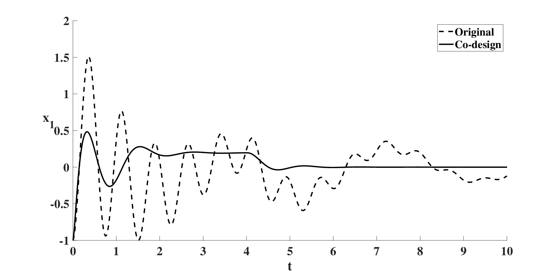
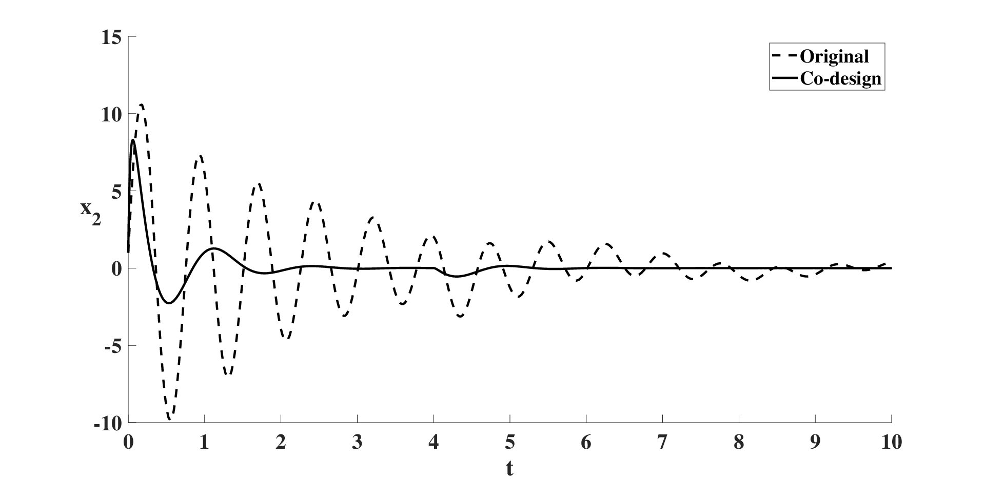
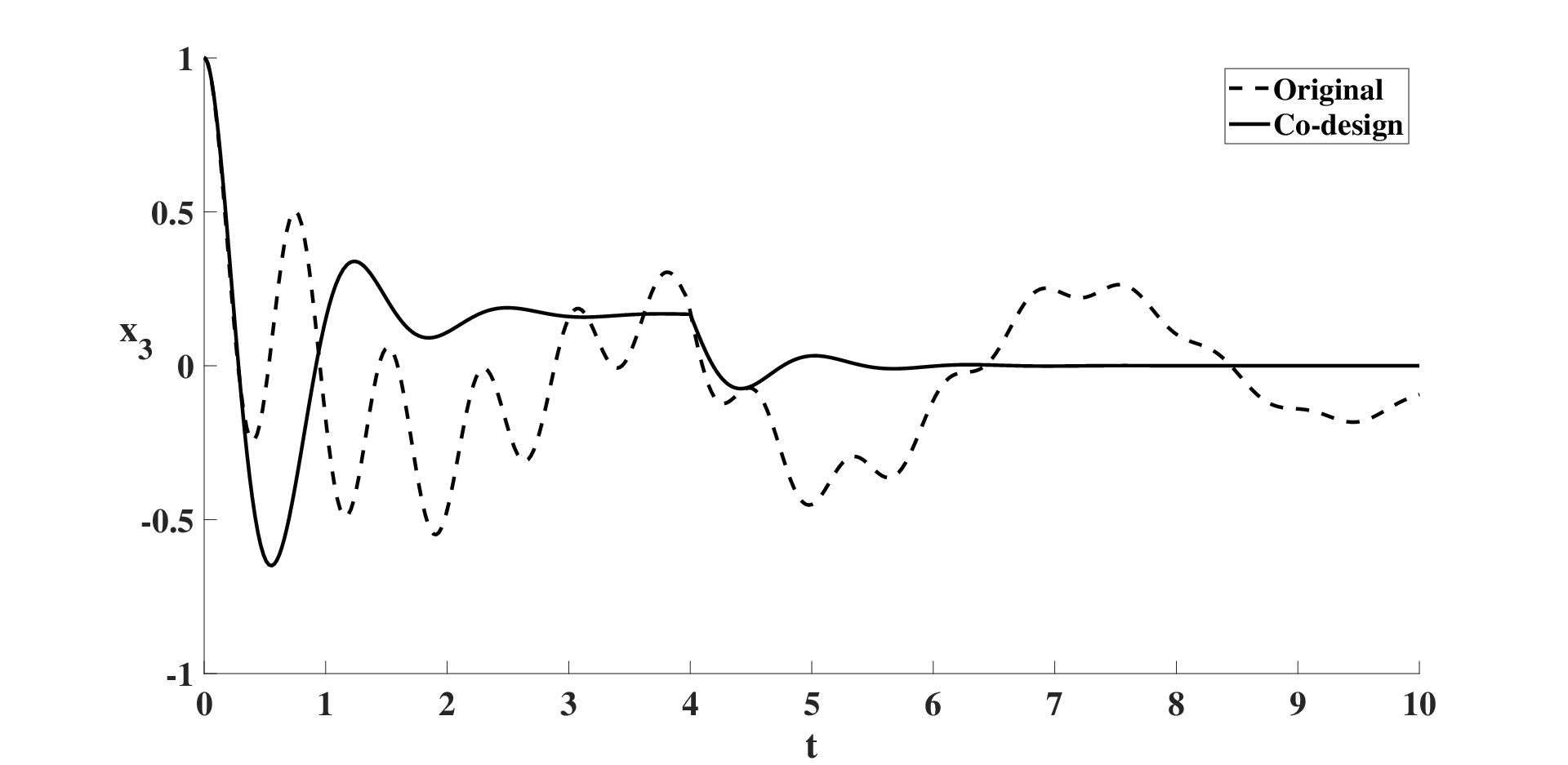
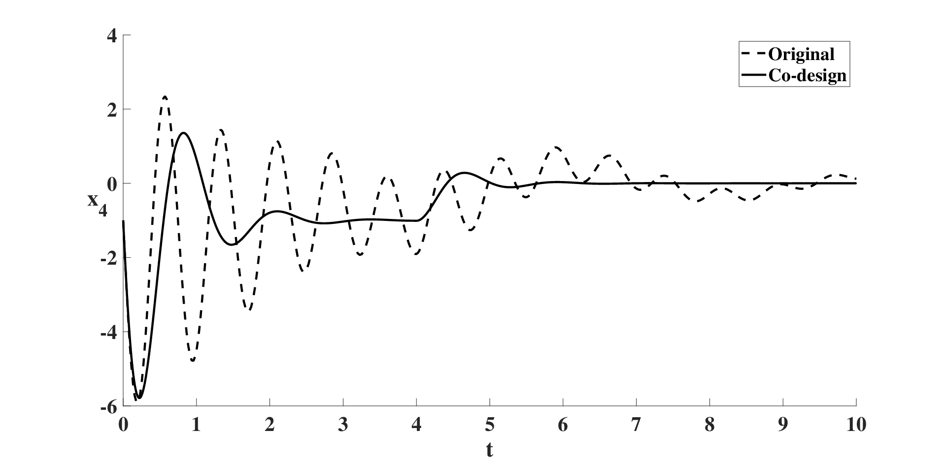
Refer to caption — (a) Evolution of $x_{1}$

We simulate the system for $w=1$ applied for the time span $0\leq t\leq 4$ with initial condition $x_{0}=\begin{pmatrix}-1&1&1&-1\end{pmatrix}^{\top}$ and show the result in Figure 2. We observe that the co-designed system shows an improvement in performance.

V Conclusion

In this letter we have studied the co-design optimization problem for systems with Lipschitz nonlinear dynamics. We propose a novel time independent reformulation of the co-design problem with a quadratic matrix equation as constraint ensuring system stability. We then propose a gradient based iterative method to compute a solution of the co-design problem. Our future work includes providing convergence and optimality guarantees to the proposed co-design solution method and extending it to general nonlinear systems.

References

[1] R. Skelton, “Model error concepts in control design,” International Journal of Control, vol. 49, no. 5, pp. 1725–1753, 1989.
[2] H. K. Fathy, J. A. Reyer, P. Y. Papalambros, and A. Ulsov, “On the coupling between the plant and controller optimization problems,” in American Control Conference, vol. 3. IEEE, 2001, pp. 1864–1869.
[3] A. L. Hale, R. J. Lisowski, and W. E. Dahl, “Optimal simultaneous structural and control design of maneuvering flexible spacecraft,” Journal of Guidance, Control, and Dynamics, vol. 8, no. 1, pp. 86–93, 1985.
[4] J. A. Reyer and P. Y. Papalambros, “Combined optimal design and control with application to an electric dc motor,” J. Mech. Des., vol. 124, no. 2, pp. 183–191, 2002.
[5] T. Ravichandran, D. Wang, and G. Heppler, “Simultaneous plant-controller design optimization of a two-link planar manipulator,” Mechatronics, vol. 16, no. 3-4, pp. 233–242, 2006.
[6] L. R. Sandoval, H. Budman, and P. Douglas, “Simultaneous design and control of processes under uncertainty: A robust modelling approach,” Journal of Process Control, vol. 18, no. 7-8, pp. 735–752, 2008.
[7] P. V. Chanekar, N. Chopra, and S. Azarm, “Optimal actuator placement for linear systems with limited number of actuators,” in American Control Conference (ACC). IEEE, 2017, pp. 334–339.
[8] ——, “Optimal structured static output feedback design using generalized benders decomposition,” in 56th Annual Conference on Decision and Control (CDC). IEEE, 2017, pp. 4819–4824.
[9] F. Lin, M. Fardad, and M. R. Jovanović, “Design of optimal sparse feedback gains via the alternating direction method of multipliers,” IEEE Transactions on Automatic Control, vol. 58, no. 9, pp. 2426–2431, 2013.
[10] P. Chanekar, E. Nozari, and J. Cortes, “Energy-transfer edge centrality and its role in enhancing network controllability,” IEEE Transactions on Network Science and Engineering, 2020.
[11] P. V. Chanekar, N. Chopra, and S. Azarm, “Co-design of linear systems using generalized benders decomposition,” Automatica, vol. 89, pp. 180–193, 2018.
[12] T. Liu, S. Azarm, and N. Chopra, “Decentralized multisubsystem co-design optimization using direct collocation and decomposition-based methods,” Journal of Mechanical Design, vol. 142, no. 9, 2020.
[13] Y. Wang and S. A. Bortoff, “Co-design of nonlinear control systems with bounded control inputs,” in 11th World Congress on Intelligent Control and Automation. IEEE, 2014, pp. 3035–3039.
[14] Y. Jiang, Y. Wang, S. A. Bortoff, and Z.-P. Jiang, “Optimal codesign of nonlinear control systems based on a modified policy iteration method,” IEEE transactions on neural networks and learning systems, vol. 26, no. 2, pp. 409–414, 2015.
[15] S. Skogestad and I. Postlethwaite, Multivariable Feedback Control: Analysis and Design. Wiley, 2005.
[16] H. K. Khalil, Nonlinear systems. Upper Saddle River, NJ: Prentice-Hall, 2002.
[17] A. Stoorvogel, “The robust ${H}_{2}$ control problem: a worst-case design,” IEEE Transactions on Automatic Control, vol. 38, no. 9, pp. 1358–1371, 1993.
[18] P. R. Pagilla and Y. Zhu, “Controller and observer design for lipschitz nonlinear systems,” in American Control Conference, vol. 3. IEEE, 2004, pp. 2379–2384.
[19] C. Aboky, G. Sallet, and J.-C. Vivalda, “Observers for lipschitz non-linear systems,” International Journal of control, vol. 75, no. 3, pp. 204–212, 2002.
[20] D. P. Bertsekas, Nonlinear Programming. Athena Scientific, 1999.
[21] T. Rautert and E. W. Sachs, “Computational design of optimal output feedback controllers,” SIAM Journal on Optimization, vol. 7, no. 3, pp. 837–852, 1997.
[22] R. A. Horn and C. R. Johnson, Matrix analysis. Cambridge university press, 2012.
[23] S. Raghavan and J. K. Hedrick, “Observer design for a class of nonlinear systems,” International Journal of Control, vol. 59, no. 2, pp. 515–528, 1994.