Cross-view Self-Supervised Learning on
Heterogeneous Graph Neural Network
via Bootstrapping
Abstract
Heterogeneous graph neural networks can represent information of heterogeneous graphs with excellent ability. Recently, self-supervised learning manner is researched which learns the unique expression of a graph through a contrastive learning method. In the absence of labels, this learning methods show great potential. However, contrastive learning relies heavily on positive and negative pairs, and generating high-quality pairs from heterogeneous graphs is difficult. In this paper, in line with recent innovations in self-supervised learning called BYOL or bootstrapping, we introduce a that can generate good representations without generating large number of pairs. In addition, paying attention to the fact that heterogeneous graphs can be viewed from two perspectives, network schema and meta-path views, high-level expressions in the graphs are captured and expressed. The proposed model showed state-of-the-art performance than other methods in various real world datasets.
Index Terms:
Heterogeneous graph neural network, Contrastive learning, Self-supervised learningI Introduction
In real world, heterogeneous graph[1] models various kinds of nodes and their relationships, such as bibliographic networks[2] or movie networks. The heterogeneous graph neural network effectively represents various relationships between these heterogeneous nodes, resulting in performance improvements in various sections, such as recommendation systems [3].
As performed in the existing general homogeneous graph neural networks[4, 5, 6], heterogeneous graph neural networks also belong to semi-supervised learning[7, 8]. Although labeling of the entire node is not required, sometimes such labeling is difficult. For example, classification of papers is difficult for non-experts. To solve this problem, self-supervised learning method was introduced[9, 10, 11, 12, 13]. The most used learning method in self-supervised learning is contrastive learning. Contrastive learning requires positive and negative pairs, and during training place embeddings of positive pairs close to each other and embeddings of negative pairs farther away. However, implementing contrastive learning on heterogeneous graphs is not an easy task.
First, high-quality contrastive learning requires a large amount of positive and negative pairs. However, in heterogeneous graphs, it is difficult to create many of these high-quality positive or negative pairs. In a typical graph, we expect neighboring nodes to have the same properties, so we can produce positive or negative pairs depending on whether they are neighbors or not. However, in heterogeneous graphs, this method may produce incorrect pairs. This is because in heterogeneous graphs, adjacent nodes with different meanings exist. For example, in a movie network, it is difficult to expect movie nodes connected via actor nodes to have the same characteristics. This is usually because actors appear in films of different characteristics. A recent study proposed BGRL[14], which improved the problem of contrastive learning. This method has been shown to enable self-supervised learning without generating large numbers of pairs, especially negative pairs.
However, this approach introduces a second problem. Since there are many non-attribute graphs in heterogeneous graphs, when augmentation of the existing attribute masking method is used, even if BGRL is used, the maximum performance is not achieved. In order to solve this problem, a new augmentation method has been proposed[15] recently, focusing on the fact that heterogeneous graphs can be viewed from two perspectives. However, these studies require two models and cannot take advantage of the BGRL. In this study, by combining the two methods, we propose a model that can express heterogeneous graphs from two perspectives while sharing trainable parameters.
- •
To the best of our knowledge, this is the first attempt to study more complex learning in BYOL in heterogeneous graphs.
- •
Our model can generate two-view node representations with a single model, which shows improved performance even in non-attribute graphs where attribute masking is useless.
- •
We perform various experiments on four real-world datasets and show that the proposed model achieved the best performance in various respects.
II Related Works
II-A Heterogeneous Graph Network
A heterogeneous graph neural network is a neural network for effectively representing a heterogeneous graph consisting of various types of nodes and links. HAN[7] uses attention at the node level and semantic level. MAGNN[8] references to intermediate nodes between nodes that are not considered in HAN through various techniques. For GTN[16], it automatically catches and uses useful connections rather than predefined ones. HGT[17] also automatically captures meaningful connections and can be easily scaled up for large datasets. HetGNN[18] samples neighbors and uses them after encoding them into LSTM. However, these neural networks do not attempt self-supervised learning.
II-B Contrastive learning
Contrastive learning refers to learning by placing embeddings of positive pairs close and embeddings of negative pairs far away, based on positive and negative pairs. In DGI[12], we learn by maximizing the amount of mutual information by using the local and global embeddings generated by the normal graph as positive pairs and the local embeddings generated by the corrupt graph and global embeddings generated by the normal graph as negative pairs. GMI[19] learns by capturing a central node within the topology and placing this node and local embeddings in positive pairs. GCC places the local embeddings of the two graphs in positive pairs. DMGI[20] conduct contrastive learning on the normal graph and the corrupt graph through the meta-path. In HeCo[15], it use different views to create positive and negative pairs through metapaths and then train them in contrast. Either they did not fully utilize the characteristics of heterogeneous graphs, or they could not produce positive or negative pairs properly.
II-C Bootstrap your own latent
To solve the problem of contrastive learning, which requires generating a large amount of positive and negative pairs, BGRL[14] has been proposed which depending on BYOL method. Self-supervised learning is performed using augmentation methods based on node masking or edge masking, and two encoders and one predictor. This method enables self-supervised learning with only positive pairs. In addition, AFGRL[21], an additional BYOL-based self-supervised learning method that does not use augmentation, has been proposed. However, in the case of BGRL, performance is poor in non-attribute graph due to the nature of reliance on masking, and in the case of AFGRL, it is difficult to reflect various types of nodes in training.
III Preliminary
III-A Heterogeneous Graph
Heterogeneous graph is defined as a . and denote sets of nodes and edges. and denotes sets of object and link types and . Finally, there are mapping functions and , which denotes for node mapping function and edge mapping function respectively.
III-B Network Schema
The network schema denoted by represents the Heterogeneous graph as a meta-template. The object is connected as a directed graph through the link type .
III-C Meta-path
A meta-path is defined as a path in the form of (abbreviated as ), which represents a composite relation between node types and , where denotes the relations composition operator.
IV Proposed Model: CSGRL
In this section, we introduce our model that encodes the nodes and then trains them through the BYOL method. As a single model, our model can represent nodes through two views: a network schema view and a meta-path view. After that, self-supervised learning is performed on two views of the same node through the BYOL method.
IV-A Encoder
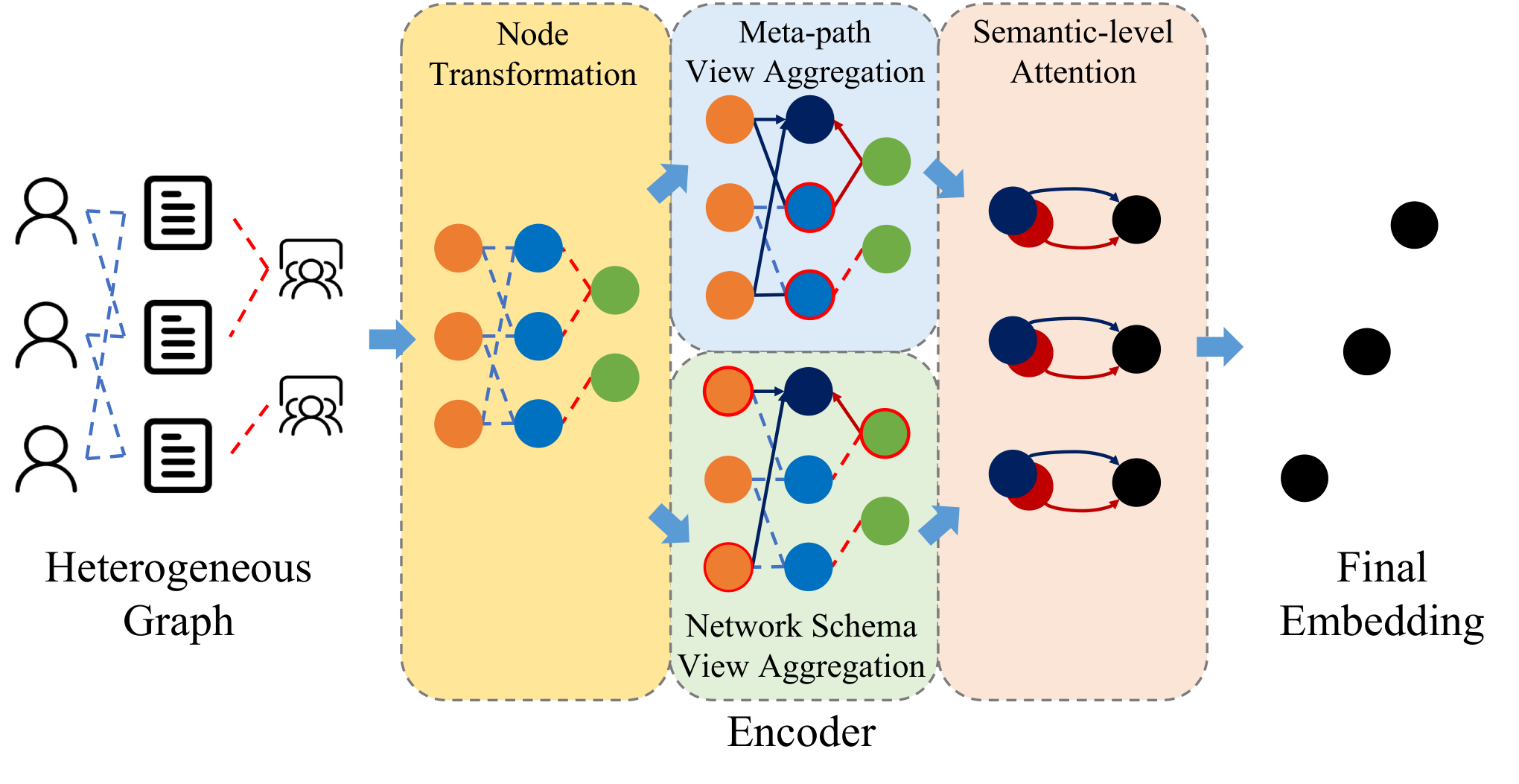
IV-A1 Node Feature Transformation
Since there are different types of nodes, we need to transform the node features in different dimension into same dimension. Converts the feature of the node with type into through each type conversion parameter, matrix and bias .
| (1) |
IV-A2 Network Schema View Aggregation
In the network schema view, node connects to nodes of different types . Among them, the neighbor node connected through the type is defined as . For example, paper is connected with neighbor nodes of author type and neighbor nodes of subject type . Aggregate by applying the RGCN[22] aggregation method. The embedding created by aggregating the type neighbors of the node is defined as:
| (2) |
IV-A3 Meta-path View Aggregation
The meta-path view aggregates neighbors connected via meta-path. For nodes, there is a meta-paths . A neighbor node of connected through each meta path is defined as . For example, if paper is connected to via author , is one of the neighbor nodes of connected via meta-path (PAP). The GCN aggregation method is used to aggregate these neighbor nodes. The embedding created by aggregating and node is defined as:
| (3) |
IV-A4 Semantic-level Attention
We aggregate the embedding generated for each meta-path or node type of node into one final embedding through attention. final embedding is defined as:
| (4) |
If meta-path view aggregate is performed, becomes , view type becomes , and when network scheme view aggregate is performed, becomes and view type becomes . The final embedding generated through the meta-path view aggregate becomes , and the final embedding generated through the network scheme view aggregate becomes . denotes importance of view type . is defined as
| (5) |
IV-B Bootstrap your own latent

IV-B1 CSGRL Component
Prepare two encoders for CSGRL training. These are the online encoder and a target encoder , respectively. Also, prepare the heterogeneous graph . After that, we use the online encoder and the target encoder to find and . We also use the predictors to find . In this process, and must be created using different view aggregate methods. That is, if is , then must be , and when is , must be .
IV-B2 Finding positive neighbors
To generate a small but high-quality positive pair, we create a set of positive neighbors for each node . is a subset of the set of all neighboring nodes connected via meta-path. Subset is created taking into count the number of meta-paths connected in . For example, add to the neighbor node of , which belongs to both and , rather than the neighbor node of that belongs only to .
IV-B3 Updating the online encoder
The online parameter (not ) is updated so that the predicted is similar to via the gradient computed via cosine similarity.
| (6) |
| (7) |
is the learning rate, and only is updated through the calculated . And we also symmetrize this loss by using the online representation of the second view to also predict the target representation of the first view.
IV-B4 Updating the target encoder
The target parameter is updated as an exponential moving average of the online parameter using the damping factor .
| (8) |
V Experiment
V-A Experimental Setup
| Dataset | Node | Relation | Meta-path |
| ACM | paper (P):4019 author (A):7167 subject (S):60 | P-A:13407 P-S:4019 | PAP PSP |
| DBLP | author (A):4057 paper (P):14328 conference (C):20 term (T):7723 | P-A:19645 P-C:14328 P-T:85810 | APA APCPA APTPA |
| Freebase | movie (M):3492 actor (A):33401 direct (D):2502 writer (W):4459 | M-A:65341 M-D:3762 M-W:6414 | MAM MDM MWM |
| AMiner | paper (P):6564 author (A):13329 reference (R):35890 | P-A:18007 P-R:58831 | PAP PRP |
| Datasets | Metric | Split | GraphSAGE | GAE | Mp2vec | HERec | HetGNN | HAN | DGI | DMGI | HeCo | CSGRL |
| ACM | Ma-F1 | 20 | 47.134.7 | 62.723.1 | 51.910.9 | 55.131.5 | 72.110.9 | 85.662.1 | 79.273.8 | 87.860.2 | 88.560.8 | 90.490.1 |
| 40 | 55.966.8 | 61.613.2 | 62.410.6 | 61.210.8 | 72.020.4 | 87.471.1 | 80.233.3 | 86.230.8 | 87.610.5 | 90.410.4 | ||
| 60 | 56.595.7 | 61.672.9 | 61.130.4 | 64.350.8 | 74.330.6 | 88.411.1 | 80.033.3 | 87.970.4 | 89.040.5 | 90.920.5 | ||
| Mi-F1 | 20 | 49.725.5 | 68.021.9 | 53.130.9 | 57.471.5 | 71.891.1 | 85.112.2 | 79.633.5 | 87.600.8 | 88.130.8 | 90.280.1 | |
| 40 | 60.983.5 | 66.381.9 | 64.430.6 | 62.620.9 | 74.460.8 | 87.211.2 | 80.413.0 | 86.020.9 | 87.450.5 | 90.340.4 | ||
| 60 | 60.724.3 | 65.712.2 | 62.720.3 | 65.150.9 | 76.080.7 | 88.101.2 | 80.153.2 | 87.820.5 | 88.710.5 | 90.780.5 | ||
| AUC | 20 | 65.883.7 | 79.502.4 | 71.660.7 | 75.441.3 | 84.361.0 | 93.471.5 | 91.472.3 | 96.720.3 | 96.490.3 | 97.360.1 | |
| 40 | 71.065.2 | 79.142.5 | 80.480.4 | 79.840.5 | 85.010.6 | 94.840.9 | 91.522.3 | 96.350.3 | 96.400.4 | 97.430.1 | ||
| 60 | 70.456.2 | 77.902.8 | 79.330.4 | 81.640.7 | 87.640.7 | 94.681.4 | 91.411.9 | 96.790.2 | 96.550.3 | 97.080.5 | ||
| DBLP | Ma-F1 | 20 | 71.978.4 | 90.900.1 | 88.980.2 | 89.570.4 | 89.511.1 | 89.310.9 | 87.932.4 | 89.940.4 | 91.280.2 | 92.560.1 |
| 40 | 73.698.4 | 89.600.3 | 88.680.2 | 89.730.4 | 88.610.8 | 88.871.0 | 88.620.6 | 89.250.4 | 90.340.3 | 91.690.1 | ||
| 60 | 73.868.1 | 90.080.2 | 90.250.1 | 90.180.3 | 89.560.5 | 89.200.8 | 89.190.9 | 89.460.6 | 90.640.3 | 92.200.1 | ||
| Mi-F1 | 20 | 71.448.7 | 91.550.1 | 89.670.1 | 90.240.4 | 90.111.0 | 90.160.9 | 88.722.6 | 90.780.3 | 91.970.2 | 93.100.1 | |
| 40 | 73.618.6 | 90.000.3 | 89.140.2 | 90.150.4 | 89.030.7 | 89.470.9 | 89.220.5 | 89.920.4 | 90.760.3 | 92.060.1 | ||
| 60 | 74.058.3 | 90.950.2 | 91.170.1 | 91.010.3 | 90.430.6 | 90.340.8 | 90.350.8 | 90.660.5 | 91.590.2 | 93.090.1 | ||
| AUC | 20 | 90.594.3 | 98.150.1 | 97.690.0 | 98.210.2 | 97.960.4 | 98.070.6 | 96.991.4 | 97.750.3 | 98.320.1 | 98.750.1 | |
| 40 | 91.424.0 | 97.850.1 | 97.080.0 | 97.930.1 | 97.700.3 | 97.480.6 | 97.120.4 | 97.230.2 | 98.060.1 | 98.680.1 | ||
| 60 | 91.733.8 | 98.370.1 | 98.000.0 | 98.490.1 | 97.970.2 | 97.960.5 | 97.760.5 | 97.720.4 | 98.590.1 | 99.070.1 | ||
| Freebase | Ma-F1 | 20 | 45.144.5 | 53.810.6 | 53.960.7 | 55.780.5 | 52.721.0 | 53.162.8 | 54.900.7 | 55.790.9 | 59.230.7 | 59.560.4 |
| 40 | 44.884.1 | 52.442.3 | 57.801.1 | 59.280.6 | 48.570.5 | 59.632.3 | 53.401.4 | 49.881.9 | 61.190.6 | 63.340.2 | ||
| 60 | 45.163.1 | 50.650.4 | 55.940.7 | 56.500.4 | 52.370.8 | 56.771.7 | 53.811.1 | 52.100.7 | 60.131.3 | 62.370.5 | ||
| Mi-F1 | 20 | 54.833.0 | 55.200.7 | 56.230.8 | 57.920.5 | 56.850.9 | 57.243.2 | 58.160.9 | 58.260.9 | 61.720.6 | 61.760.5 | |
| 40 | 57.083.2 | 56.052.0 | 61.011.3 | 62.710.7 | 53.961.1 | 63.742.7 | 57.820.8 | 54.281.6 | 64.030.7 | 65.440.2 | ||
| 60 | 55.923.2 | 53.850.4 | 58.740.8 | 58.570.5 | 56.840.7 | 61.062.0 | 57.960.7 | 56.691.2 | 63.611.6 | 64.650.5 | ||
| AUC | 20 | 67.635.0 | 73.030.7 | 71.780.7 | 73.890.4 | 70.840.7 | 73.262.1 | 72.800.6 | 73.191.2 | 76.220.8 | 76.400.1 | |
| 40 | 66.424.7 | 74.050.9 | 75.510.8 | 76.080.4 | 69.480.2 | 77.741.2 | 72.971.1 | 70.771.6 | 78.440.5 | 78.480.7 | ||
| 60 | 66.783.5 | 71.750.4 | 74.780.4 | 74.890.4 | 71.010.5 | 75.691.5 | 73.320.9 | 73.171.4 | 78.040.4 | 78.130.4 | ||
| AMiner | Ma-F1 | 20 | 42.462.5 | 60.222.0 | 54.780.5 | 58.321.1 | 50.060.9 | 56.073.2 | 51.613.2 | 59.502.1 | 71.381.1 | 76.340.2 |
| 40 | 45.771.5 | 65.661.5 | 64.770.5 | 64.500.7 | 58.970.9 | 63.851.5 | 54.722.6 | 61.922.1 | 73.750.5 | 80.400.6 | ||
| 60 | 44.912.0 | 63.741.6 | 60.650.3 | 65.530.7 | 57.341.4 | 62.021.2 | 55.452.4 | 61.152.5 | 75.801.8 | 80.220.1 | ||
| Mi-F1 | 20 | 49.683.1 | 65.782.9 | 60.820.4 | 63.641.1 | 61.492.5 | 68.864.6 | 62.393.9 | 63.933.3 | 78.811.3 | 83.080.2 | |
| 40 | 52.102.2 | 71.341.8 | 69.660.6 | 71.570.7 | 68.472.2 | 76.891.6 | 63.872.9 | 63.602.5 | 80.530.7 | 86.720.9 | ||
| 60 | 51.362.2 | 67.701.9 | 63.920.5 | 69.760.8 | 65.612.2 | 74.731.4 | 63.103.0 | 62.512.6 | 82.461.4 | 86.320.1 | ||
| AUC | 20 | 70.862.5 | 85.391.0 | 81.220.3 | 83.350.5 | 77.961.4 | 78.922.3 | 75.892.2 | 85.340.9 | 90.820.6 | 93.090.8 | |
| 40 | 74.441.3 | 88.291.0 | 88.820.2 | 88.700.4 | 83.141.6 | 80.722.1 | 77.862.1 | 88.021.3 | 92.110.6 | 93.860.3 | ||
| 60 | 74.161.3 | 86.920.8 | 85.570.2 | 87.740.5 | 84.770.9 | 80.391.5 | 77.211.4 | 86.201.7 | 92.400.7 | 95.280.1 |


V-A1 Datasets
We use four real datasets. ACM[23] is an academic network. The object of classification is papers, and there are three classes. DBLP[8] is also an academic network. The object of classification is the paper, and there are four classes. Freebase[24] is a film information network. The object of classification is movies and is divided into three classes. AMiner[25] is an academic network, divided into four classes.
V-A2 Baselines
V-A3 Implementation Detail
For random walk-based methods, the number of walks is set to , the length is , and the window size is set to . For other parameters, follow the settings of the original document. Experimental results refer to those of HeCo. For CSGRL, the learning rate is set to and weight decay is set to . To perform mini-batch training, HGT mini-batch method is used. The batch size is set to . The optimization function uses AdamW. It is set to for in BYOL.
| Datasets | ACM | DBLP | Freebase | AMiner | ||||
| Metrics | NMI | ARI | NMI | ARI | NMI | ARI | NMI | ARI |
| GraphSage | 29.20 | 27.72 | 51.50 | 36.40 | 9.05 | 10.49 | 15.74 | 10.10 |
| GAE | 27.42 | 24.49 | 72.59 | 77.31 | 19.03 | 14.10 | 28.58 | 20.90 |
| Mp2vec | 48.43 | 34.65 | 73.55 | 77.70 | 16.47 | 17.32 | 30.80 | 25.26 |
| HERec | 47.54 | 35.67 | 70.21 | 73.99 | 19.76 | 19.36 | 27.82 | 20.16 |
| HetGNN | 41.53 | 34.81 | 69.79 | 75.34 | 12.25 | 15.01 | 21.46 | 26.60 |
| DGI | 51.73 | 41.16 | 59.23 | 61.85 | 18.34 | 11.29 | 22.06 | 15.93 |
| DMGI | 51.66 | 46.64 | 70.06 | 75.46 | 16.98 | 16.91 | 19.24 | 20.09 |
| HeCo | 56.87 | 56.94 | 74.51 | 80.17 | 20.38 | 20.98 | 32.26 | 28.64 |
| CSGRL | 66.13 | 70.84 | 74.88 | 80.24 | 22.76 | 22.81 | 44.45 | 39.25 |
| Datasets | ACM | AMiner | ||||
| Metrics | Ma-F1 | Mi-F1 | AUC | Ma-F1 | Mi-F1 | AUC |
| BGRL | 90.430.2 | 90.260.2 | 97.050.1 | 64.280.9 | 70.361.1 | 87.900.3 |
| CSGRL-wopp | 90.510.3 | 90.370.3 | 97.150.1 | 73.540.4 | 80.650.4 | 92.48±0.1 |
| CSGRL | 90.920.5 | 90.780.5 | 97.080.5 | 80.220.1 | 86.320.1 | 95.280.1 |
V-B Node Classification
The learned embeddings are used to train the linear classifier. Assuming there are 20, 40, or 60 labeled nodes for each class as training set. For each dataset, 1000 is set as the validation set and 1000 as the test set. We use common evaluation metrics such as Macro-F1, Micro-F1, AUC. Referring to Table II, In all cases, our model outperformed other competing models, indicating that the BYOL approach is effective for unsupervised learning.
V-C Node Clustering
In this task, we compute and report the NMI and ARI using the K-means algorithm for learned embeddings. Referring to Table III, It also outperforms other competing models in node clustering.
V-D Node Visualization
To provide a more intuitive assessment, we provide embedding visualizations for ACM. Comparison with Mp2vec, DGI, DMGI, HeCo using T-SNE. In Figure 3, embeddings are clearly separated by class, and the silhouette score is higher than that of other comparative models, indicating that embeddings were successful.
V-E Analysis with CSGRL variant
Referring to Table IV, it can be seen that the performance of BGRL and CSGRL is similar in the case of ACM, which is a dataset with attributes, but the performance of BGRL is not good in the case of AMiner, which is a non-attribute dataset. For CSGRL-wopp, a model trained without positive pairs, we can observe that the performance is comparable to or worse than CSGRL. Here, we prove that using a positive pair is effective for improving performance.
VI Conclusion
In this paper, we propose a self-supervised heterogeneous graph neural network called CSGRL using a BYOL methodology and enhanced augmentation methods. CSGRL learns how to efficiently represent complex information using two views: network schema and meta-path. We also use the BYOL methodology to avoid the problem of finding positive and negative pairs, one of the major difficulties that exist in self-supervised heterogeneous graph learning. In extensive experiments, it has been proven that our model outperforms other models.
References
- [1] Y. Sun and J. Han, “Mining heterogeneous information networks: a structural analysis approach,” SIGKDD Explor., pp. 20–28, 2012.
- [2] W. Hu, B. Liu, J. Gomes, M. Zitnik, P. Liang, V. S. Pande, and J. Leskovec, “Strategies for pre-training graph neural networks,” in ICLR, 2020.
- [3] C. Shi, B. Hu, W. X. Zhao, and P. S. Yu, “Heterogeneous information network embedding for recommendation,” IEEE Trans. Knowl. Data Eng., pp. 357–370, 2019.
- [4] T. N. Kipf and M. Welling, “Semi-supervised classification with graph convolutional networks,” in ICLR, 2017.
- [5] P. Velickovic, G. Cucurull, A. Casanova, A. Romero, P. Liò, and Y. Bengio, “Graph attention networks,” in ICLR, 2018.
- [6] W. L. Hamilton, Z. Ying, and J. Leskovec, “Inductive representation learning on large graphs,” in NeurIPS, 2017, pp. 1024–1034.
- [7] X. Wang, H. Ji, C. Shi, B. Wang, Y. Ye, P. Cui, and P. S. Yu, “Heterogeneous graph attention network,” in WWW, 2019, pp. 2022–2032.
- [8] X. Fu, J. Zhang, Z. Meng, and I. King, “MAGNN: metapath aggregated graph neural network for heterogeneous graph embedding,” in WWW, 2020, pp. 2331–2341.
- [9] A. v. d. Oord, Y. Li, and O. Vinyals, “Representation learning with contrastive predictive coding,” arXiv preprint arXiv:1807.03748, 2018.
- [10] K. He, H. Fan, Y. Wu, S. Xie, and R. B. Girshick, “Momentum contrast for unsupervised visual representation learning,” in CVPR, 2020, pp. 9726–9735.
- [11] T. Chen, S. Kornblith, M. Norouzi, and G. E. Hinton, “A simple framework for contrastive learning of visual representations,” in ICML, 2020, pp. 1597–1607.
- [12] P. Velickovic, W. Fedus, W. L. Hamilton, P. Liò, Y. Bengio, and R. D. Hjelm, “Deep graph infomax,” in ICLR, 2019.
- [13] K. Hassani and A. H. K. Ahmadi, “Contrastive multi-view representation learning on graphs,” in ICML, 2020, pp. 4116–4126.
- [14] S. Thakoor, C. Tallec, M. G. Azar, R. Munos, P. Velickovic, and M. Valko, “Bootstrapped representation learning on graphs,” CoRR, vol. abs/2102.06514, 2021.
- [15] X. Wang, N. Liu, H. Han, and C. Shi, “Self-supervised heterogeneous graph neural network with co-contrastive learning,” in KDD ’21: The 27th ACM SIGKDD Conference on Knowledge Discovery and Data Mining, Virtual Event, Singapore, August 14-18, 2021, 2021, pp. 1726–1736.
- [16] S. Yun, M. Jeong, R. Kim, J. Kang, and H. J. Kim, “Graph transformer networks,” in NeurIPS, 2019, pp. 11 960–11 970.
- [17] Z. Hu, Y. Dong, K. Wang, and Y. Sun, “Heterogeneous graph transformer,” in WWW, 2020, pp. 2704–2710.
- [18] C. Zhang, D. Song, C. Huang, A. Swami, and N. V. Chawla, “Heterogeneous graph neural network,” in SIGKDD, 2019, pp. 793–803.
- [19] Z. Peng, W. Huang, M. Luo, Q. Zheng, Y. Rong, T. Xu, and J. Huang, “Graph representation learning via graphical mutual information maximization,” in WWW, 2020, pp. 259–270.
- [20] C. Park, D. Kim, J. Han, and H. Yu, “Unsupervised attributed multiplex network embedding,” in AAAI, 2020, pp. 5371–5378.
- [21] N. Lee, J. Lee, and C. Park, “Augmentation-free self-supervised learning on graphs,” CoRR, vol. abs/2112.02472, 2021.
- [22] M. S. Schlichtkrull, T. N. Kipf, P. Bloem, R. van den Berg, I. Titov, and M. Welling, “Modeling relational data with graph convolutional networks,” in ESWC, 2018, pp. 593–607.
- [23] J. Zhao, X. Wang, C. Shi, Z. Liu, and Y. Ye, “Network schema preserving heterogeneous information network embedding,” in IJCAI, 2020, pp. 1366–1372.
- [24] X. Li, D. Ding, B. Kao, Y. Sun, and N. Mamoulis, “Leveraging meta-path contexts for classification in heterogeneous information networks,” arXiv preprint arXiv:2012.10024, 2020.
- [25] B. Hu, Y. Fang, and C. Shi, “Adversarial learning on heterogeneous information networks,” in SIGKDD, 2019, pp. 120–129.
- [26] T. N. Kipf and M. Welling, “Variational graph auto-encoders,” arXiv preprint arXiv:1611.07308, 2016.
- [27] Y. Dong, N. V. Chawla, and A. Swami, “metapath2vec: Scalable representation learning for heterogeneous networks,” in SIGKDD, 2017, pp. 135–144.