跳到论文正文
W Papers独立论文阅读器 arXiv:2201.03136 论文正文 计算阅读时间 · 0%
引用这篇论文根据当前论文元数据生成,正式投稿前建议核对。


License: CC BY-NC-SA 4.0
arXiv:2201.03136v1 [eess.SY] 10 Jan 2022

Data-driven Output-feedback Predictive Control:
Unknown Plant’s Order and Measurement Noisefootnoteinfo

Nam H. Jo Email: nhjo@ssu.ac.kr    Hyungbo Shim Email: hshim@snu.ac.kr
Abstract

The aim of this paper is to propose a new data-driven control scheme for multi-input-multi-output linear time-invariant systems whose system model are completely unknown. Using a non-minimal input-output realization, the proposed method can be applied to the case where the system order is unknown, provided that its upper bound is known. A workaround against measurement noise is proposed and it is shown through simulation study that the proposed method is superior to the conventional methods when dealing with input/output data corrupted by measurement noise.

keywords
data-driven control, predictive control, uncertain systems, unknown order, Moore-Penrose inverse
††thanks: [††address: Department of Electrical Engineering, Soongsil University, Seoul, Korea††address: ASRI, Department of Electrical and Computer Engineering, Seoul National University, Seoul, Korea

footnoteinfo]This work was supported by the National Research Foundation of Korean(NRF) grant funded by the Korea government(MIST) (No. 2020R1F1A1069426), and by AI based Flight Control Research Laboratory funded by Defense Acquisition Program Administration under Grant UD200045CD.

and

1 Introduction

Obtaining a mathematical model is the first step for model-based control designs, which has been however a difficulty in some applications. This has motivated the study of model-free, data-driven control methods, and recently a method called Data-enabled Predictive Control (abbreviated by DeePC) is presented by Coulson et al. 2019. The root of DeePC is the classical Model Predictive Control (MPC). By noting that, at each sampling time, MPC finds an optimal control sequence for a finite time interval by evaluating a cost function based on the output sequence generated by a mathematical system model, DeePC simply replaces the model-based output sequence with a linear combination of the output data which are measured and stored from the previous experiments. This replacement is justified by the celebrated behavioral approach by Willems et al. 2005.

While DeePC has been successfully applied to several practices, some limitations are found from a few examples. A limitation arises when an unstable system is the target of the control and the optimization horizon for MPC is not short. In this case, the length of output data is not short, and hence, exponentially growing output data tend to cause numerical errors in optimization. Another limitation is that, when the output is measured under a noisy environment, we have often witnessed that DeePC does not yield satisfactory performances, even with the regularization proposed in (Coulson et al. 2019).

As an alternative, we propose to employ the data-driven system representation by De Persis & Tesi 2019. More specifically, the predicted output sequence for optimization at each sampling time is generated by the system equation, which is represented by the collected input/output data. We will see in Section 5 that the outcomes of this approach yield quite different output responses from those using DeePC under measurement noises.

However, employing the approach of (De Persis & Tesi 2019) to our purpose was not straightforward, and therefore, the contribution of this paper lies in the following points:

  1. 1.

    The approach of (De Persis & Tesi 2019) requires the knowledge of system order nn. This may make sense when we can measure the system state in that the size of the state vector is the system order. However, since our interest is a completely model-free control, asking the knowledge of system order nn may be too much because it is a part of model information. Our first contribution is to prove that the knowledge of nn is not necessary.

  2. 2.

    The way of handling multi-input-multi-output (MIMO) system in (De Persis & Tesi 2019) has a limitation (see Remark 5). Our second contribution is to present an idea of handling MIMO system as a multi-channel MISO (multi-input-single-output) system. In this case, the multi-channel MISO system cannot be realized as the minimal order in general, but thanks to the derivation of the item (1) above, we can handle non-minimal order of system representation. This idea enables the proposed method applicable to any MIMO systems without any limitation.

  3. 3.

    Our third contribution is a finding that the effect of measurement noise can be efficiently relieved by averaging the data-driven model of the system and by intentionally taking unnecessarily large n¯\bar{n} (the estimated upper bound of system order). This effect will be observed in Section 5.

Notation: For a set of vectors u1,…,uNu_{1},\dots,u_{N}, we let col​(u1,…,uN):=[u1T,…,uNT]T\text{col}(u_{1},\dots,u_{N}):=[u_{1}^{T},\dots,u_{N}^{T}]^{T}. Given a discrete-time signal u:ℤ→ℝmu:{\mathbb{Z}}\to{\mathbb{R}}^{m}, col(u⁡(a),…,u⁡(b))(u(a),\dots,u(b)) is represented by u[a,b]u_{[a,b]}. The Kronecker product is written as ⊗\otimes. The norm ‖u‖R2\|u\|_{R}^{2} denotes the quadratic form uT​R​uu^{T}Ru. The n×nn\times n identity matrix is denoted by InI_{n} (or II when no confusion is possible), and the n×mn\times m zero matrix is denoted by 0n×m0_{n\times m}. A vector [0,0,…,0,1,0,…,0]T[0,0,\dots,0,1,0,\dots,0]^{T} with the entry 11 in the ii-th place is denoted by eie_{i}. For a matrix AA, A†A^{\dagger} denotes the Moore-Penrose inverse of AA.

2 Problem Formulation and MPC

We consider a discrete-time linear time-invariant system

x⁡(t+1)=A​x​(t)+B​u​(t),y⁡(t)=C​x​(t)\displaystyle\begin{split}x(t+1)&=Ax(t)+Bu(t),\quad y(t)=Cx(t)\end{split} (1)

where A∈ℝn×nA\in{\mathbb{R}}^{n\times n}, B∈ℝn×mB\in{\mathbb{R}}^{n\times m}, C∈ℝp×nC\in{\mathbb{R}}^{p\times n}, and x⁡(t)∈ℝnx(t)\in{\mathbb{R}}^{n}, u⁡(t)∈ℝmu(t)\in{\mathbb{R}}^{m}, y⁡(t)∈ℝpy(t)\in{\mathbb{R}}^{p} are the state, the control input, and the output at time tt, respectively. It is assumed that system (1) is controllable and observable. Given a reference r⁡(t)∈ℝpr(t)\in{\mathbb{R}}^{p}, an input constraint set 𝒰⊂ℝm{\mathcal{U}}\subset{\mathbb{R}}^{m}, and an output constraint set 𝒴⊂ℝp{\mathcal{Y}}\subset{\mathbb{R}}^{p}, our goal is to build an output feedback controller such that y⁡(t)y(t) tracks r⁡(t)r(t) while satisfying the input and output constraints. This goal should be achieved without the knowledge of system matrices AA, BB, CC, and the system order nn.

Assumption 1

The unknown system order nn belongs to a given interval [1,n¯][1,\bar{n}] where n¯∈ℤ\bar{n}\in{\mathbb{Z}} is known. ◇\Diamond

The assumption is easily met in many cases by taking sufficiently large n¯\bar{n}.

When the system model (1) is known, the goal is achievable straightforwardly by the model predictive control (MPC) with a state observer; that is, at each time tt, get an estimate x^​(t)\hat{x}(t) of the state, solve the optimization problem:

minu¯\displaystyle\min_{\bar{u}}\ \ ∑k=0N−1(‖y¯k−r⁡(t+k)‖Q2+‖u¯k‖R2)\displaystyle\sum_{k=0}^{N-1}\left(\|\bar{y}_{k}-r(t+k)\|_{Q}^{2}+\|\bar{u}_{k}\|_{R}^{2}\right) (2a)
subject to x¯k+1=A​x¯k+B​u¯k,y¯k=C​x¯k\displaystyle\bar{x}_{k+1}=A\bar{x}_{k}+B\bar{u}_{k},\ \bar{y}_{k}=C\bar{x}_{k} (2b)
x¯0=x^​(t)\displaystyle\bar{x}_{0}=\hat{x}(t) (2c)
u¯k∈𝒰,y¯k∈𝒴,k=0,1,…,N−1\displaystyle\bar{u}_{k}\in{\mathcal{U}},\ \bar{y}_{k}\in{\mathcal{Y}},\ k=0,1,\dots,N-1 (2d)

where N∈ℤ>0N\in{\mathbb{Z}}_{>0} is the time horizon, u¯=col⁡(u¯0,…,u¯N−1)\bar{u}={\rm col}(\bar{u}_{0},\dots,\bar{u}_{N-1}), Q∈ℝp×pQ\in{\mathbb{R}}^{p\times p} and R∈ℝm×mR\in{\mathbb{R}}^{m\times m} are positive semi-definite and positive definite matrices, respectively, and apply u⁡(t)=u¯0u(t)=\bar{u}_{0} to the plant (1) at time tt.

Remark 1.

To ensure asymptotic convergence of (y⁡(t)−r⁡(t))(y(t)-r(t)) to zero, we need a reference input ur​(t)u_{r}(t) that satisfies xr​(t+1)=A​xr​(t)+B​ur​(t)x_{r}(t+1)=Ax_{r}(t)+Bu_{r}(t) and r⁡(t)=C​xr​(t)r(t)=Cx_{r}(t), ∀t≥0\forall t\geq 0, with some trajectory xr​(t)x_{r}(t), and the term ‖u¯k‖R2\|\bar{u}_{k}\|_{R}^{2} in the cost function in (2a) needs to be replaced with ‖u¯k−ur​(t+k)‖R2\|\bar{u}_{k}-u_{r}(t+k)\|_{R}^{2}. However, computing uru_{r} is not always easy in the model-free setting, and thus, uru_{r} is often ignored in the literature.

3 Review of DeePC

Data-enabled Predictive Control (DeePC) is firstly introduced in (Coulson et al. 2019), which is a neat and simple approach for model-free MPC. Suppose that the system model (1) is unknown but input/output data samples are available. The following definition is a key to the forthcoming discussions.

Definition 2.

The signal u[0,T−1]∈ℝm​Tu_{[0,T-1]}\in{\mathbb{R}}^{mT} is persistently exciting of order LL if the Hankel matrix

ℋL​(u):=[u⁡(0)u⁡(1)⋯u⁡(T−L)u⁡(1)u⁡(2)⋯⋯u⁡(L−1)u⁡(L)⋯u⁡(T−1)]{\mathcal{H}}_{L}(u):=\begin{bmatrix}u(0)&u(1)&\cdots&u(T-L)\\ u(1)&u(2)&\cdots&\\ \vdots&&\cdots&\\ u(L-1)&u(L)&\cdots&u(T-1)\end{bmatrix}

has full row rank.

Note that, if uu is persistently exciting of order LL, then it is also persistently exciting of order L~\tilde{L} for any L~≤L\tilde{L}\leq L. Moreover, for a signal uu to be persistently exciting of order LL, it is necessary that T≥(m+1)​L−1T\geq(m+1)L-1.

In order to introduce DeePC algorithm, let TT, TiniT_{\rm ini}, N∈ℤ+N\in{\mathbb{Z}}_{+} be given such that T≥(m+1)​(Tini+N+n)−1T\geq(m+1)(T_{\rm ini}+N+n)-1. We also let ud=col​(ud​(0),⋯,ud​(T−1))u_{d}=\text{col}(u_{d}(0),\cdots,u_{d}(T-1)) be a sequence of TT inputs applied to system (1), and yd=col​(yd​(0),⋯,yd​(T−1))y_{d}=\text{col}(y_{d}(0),\cdots,y_{d}(T-1)) be the corresponding outputs. Here, the subscript dd indicates that it is the sample data collected offline from pre-experiments. Define

[UpUf]:=ℋTini+N​(ud),[YpYf]:=ℋTini+N​(yd)\displaystyle\begin{bmatrix}U_{p}\\ U_{f}\end{bmatrix}:={\mathcal{H}}_{T_{\rm ini}+N}(u_{d}),\ \begin{bmatrix}Y_{p}\\ Y_{f}\end{bmatrix}:={\mathcal{H}}_{T_{\rm ini}+N}(y_{d})

where UpU_{p} consists of the first TiniT_{\rm ini} block rows of ℋTini+N​(ud){\mathcal{H}}_{T_{\rm ini}+N}(u_{d}) and UfU_{f} consists of the last NN block rows of ℋTini+N​(ud){\mathcal{H}}_{T_{\rm ini}+N}(u_{d}) (YpY_{p} and YfY_{f} are defined similarly). Then, by the Fundamental Lemma (Willems et al. 2005), there exists a vector g∈ℝT−Tini−N+1g\in{\mathbb{R}}^{T-T_{\rm ini}-N+1} such that

[UpYpUfYf]​g=[u[−Tini,−1]y[−Tini,−1]u[0,N−1]y[0,N−1]],\begin{bmatrix}U_{p}\\ Y_{p}\\ U_{f}\\ Y_{f}\end{bmatrix}g=\begin{bmatrix}u_{[-T_{\rm ini},-1]}\\ y_{[-T_{\rm ini},-1]}\\ u_{[0,N-1]}\\ y_{[0,N-1]}\end{bmatrix},

if udu_{d} is persistently exciting of order Tini+N+nT_{\rm ini}+N+n. This implies that the system outputs y[0,N−1]y_{[0,N-1]} can be computed provided that ud,yd,u[−Tini,−1],y[−Tini,−1]u_{d},y_{d},u_{[-T_{\rm ini},-1]},y_{[-T_{\rm ini},-1]} and u[0,N−1]u_{[0,N-1]} are given. In other words, future outputs y[0,N−1]y_{[0,N-1]} can be predicted without the knowledge of system model (1). Consider the optimization problem:

ming∑k=0N−1(‖y¯k−r⁡(t+k)‖Q2+‖u¯k‖R2)subject to[UpYpUfYf]​g=[uiniyiniu¯y¯]uini=col​(u⁡(t−Tini),⋯,u⁡(t−1)),yini=col​(y⁡(t−Tini),⋯,y⁡(t−1)),u¯k∈𝒰,k=0,⋯,N−1y¯k∈𝒴,k=0,⋯,N−1,\displaystyle\begin{split}\min_{g}\ \ &\sum_{k=0}^{N-1}\left(\|\bar{y}_{k}-r(t+k)\|_{Q}^{2}+\|\bar{u}_{k}\|_{R}^{2}\right)\\ \text{subject to}\ \ &\begin{bmatrix}U_{p}\\ Y_{p}\\ U_{f}\\ Y_{f}\end{bmatrix}g=\begin{bmatrix}u_{\rm ini}\\ y_{\rm ini}\\ \bar{u}\\ \bar{y}\end{bmatrix}\\ &u_{\rm ini}=\text{col}(u(t-T_{\rm ini}),\cdots,u(t-1)),\\ &y_{\rm ini}=\text{col}(y(t-T_{\rm ini}),\cdots,y(t-1)),\\ &\bar{u}_{k}\in{\mathcal{U}},\ k=0,\cdots,N-1\\ &\bar{y}_{k}\in{\mathcal{Y}},\ k=0,\cdots,N-1,\end{split} (3)

where u¯=col​(u¯0,⋯,u¯N−1)\bar{u}=\text{col}(\bar{u}_{0},\cdots,\bar{u}_{N-1}) and y¯=col​(y¯0,⋯,y¯N−1)\bar{y}=\text{col}(\bar{y}_{0},\cdots,\bar{y}_{N-1}). The DeePC algorithm is described as follows: at time t−1t-1, the output y⁡(t−1)y(t-1) is measured, and construct uiniu_{\rm ini} and yiniy_{\rm ini} with u⁡(t−1)u(t-1). Solve the above optimization problem, get u¯=Uf​g\bar{u}=U_{f}g with the optimal solution gg, and apply u⁡(t)=u¯0u(t)=\bar{u}_{0} at time tt.

To apply the DeePC algorithm to the case where the plant output is subject to measurement noise, the regularized DeePC (let us call it as rDeePC) is introduced based on the following optimization problem (Coulson et al. 2019; Elokda et al. 2019; Berberich et al. 2020):

ming,σy∑k=0N−1(CLOSE\displaystyle\min_{g,\sigma_{y}}\ \ \sum_{k=0}^{N-1}\big( OPEN‖y¯k−r⁡(t+k)‖Q2+‖u¯k‖R2)+λg​‖g‖2+λy​‖σy‖2\displaystyle\|\bar{y}_{k}-r(t+k)\|_{Q}^{2}+\|\bar{u}_{k}\|_{R}^{2}\big)+\lambda_{g}\|g\|^{2}+\lambda_{y}\|\sigma_{y}\|^{2}
subject to [UpYpUfYf]​g=[uiniyini+σyu¯y¯]\displaystyle\begin{bmatrix}U_{p}\\ Y_{p}\\ U_{f}\\ Y_{f}\end{bmatrix}g=\begin{bmatrix}u_{\rm ini}\\ y_{\rm ini}+\sigma_{y}\\ \bar{u}\\ \bar{y}\end{bmatrix} (4)
uini=col​(u⁡(t−Tini),⋯,u⁡(t−1)),\displaystyle u_{\rm ini}=\text{col}(u(t-T_{\rm ini}),\cdots,u(t-1)),
yini=col​(y⁡(t−Tini),⋯,y⁡(t−1)),\displaystyle y_{\rm ini}=\text{col}(y(t-T_{\rm ini}),\cdots,y(t-1)),
u¯k∈𝒰,k=0,⋯,N−1,\displaystyle\bar{u}_{k}\in{\mathcal{U}},\ k=0,\cdots,N-1,
y¯k∈𝒴,k=0,⋯,N−1,\displaystyle\bar{y}_{k}\in{\mathcal{Y}},\ k=0,\cdots,N-1,

where σy∈ℝp​Tini\sigma_{y}\in{\mathbb{R}}^{pT_{\rm ini}} is a slack variable, and λy,λg∈ℝ\lambda_{y},\lambda_{g}\in{\mathbb{R}} are regularization parameters. Although the performance of rDeePC relies on the selection of λg\lambda_{g} and λy\lambda_{y}, there is no systematic way to appropriately choose them.

4 Data-Driven Predictive Control (D2PC)

Data-enabled Predictive Control (DeePC) is a simple approach for model-free MPC and it has been successfully applied to several practices. However, it often does not yield satisfactory performances when an unstable system is to be controlled or the output is measured under a noisy environment, even if the regularized DeePC (Coulson et al. 2019; Elokda et al. 2019; Berberich et al. 2020) is employed.

As an alternative, one may build a system model (1) from the experimental data, and plug the model in (2). For the purpose of building a data-driven model, we employ the recent approach by De Persis & Tesi 2019. Elimination of the use of state observer in the MPC (2) is also from the idea of (De Persis & Tesi 2019, Section VI). Let us call this strategy by Data-Driven Predictive Control (D2PC). However, this idea confronts an immediate difficulty that the plant order nn should be known in (De Persis & Tesi 2019). In this section, we briefly review the model building by De Persis & Tesi 2019 and present how to overcome the difficulty.

4.1 Data-driven representation of input and output: SISO case

We first consider (1) in the case of single-input-single-output (SISO); i.e., m=p=1m=p=1. In this case, the input uu and the output yy of (1) obeys

y(t)=−∑j=1najy(t−j)+∑j=1nbju(t−j)\displaystyle y(t)=-\sum_{j=1}^{n}a_{j}y(t-j)+\sum_{j=1}^{n}b_{j}u(t-j) (5)

where the coefficients satisfy

zn+a1​zn−1+⋯+an=det(z​I−A)b1​zn−1+⋯+bn=det([z​I−A−BC0]).\displaystyle\begin{split}z^{n}+a_{1}z^{n-1}+\dots+a_{n}=\det(zI-A)\\ b_{1}z^{n-1}+\dots+b_{n}=\det\left(\begin{bmatrix}zI-A&\;\;-B\\ C&0\end{bmatrix}\right).\end{split} (6)

Define a vector χ∈ℝ2​n\chi\in{\mathbb{R}}^{2n} as

χ​(t):=col​(CLOSE\displaystyle\chi(t):=\text{col}( y⁡(t−n),y⁡(t−n+1),…,y⁡(t−1),\displaystyle y(t-n),y(t-n+1),\dots,y(t-1),
OPENu⁡(t−n),u⁡(t−n+1),…,u⁡(t−1))\displaystyle u(t-n),u(t-n+1),\dots,u(t-1))

which is available to the controller for all t≥nt\geq n because yy is measured and uu is generated by the controller. Then, it is seen that

χ⁡(t+1)=𝒜​χ​(t)+ℬ​u​(t),y⁡(t)=𝒞​χ​(t)\displaystyle\begin{split}\chi(t+1)&={\mathcal{A}}\chi(t)+{\mathcal{B}}u(t),\quad y(t)={\mathcal{C}}\chi(t)\end{split} (7)

where 𝒜∈ℝ2​n×2​n{\mathcal{A}}\in{\mathbb{R}}^{2n\times 2n}, ℬ∈ℝ2​n×1{\mathcal{B}}\in{\mathbb{R}}^{2n\times 1}, and 𝒞∈ℝ1×2​n{\mathcal{C}}\in{\mathbb{R}}^{1\times 2n} are

𝒜\displaystyle{\mathcal{A}} =[01…000…000…000…000…100…0−an−an−1…−a1bnbn−1…b100…001…000…000…000…000…100…000…0]\displaystyle=\begin{bmatrix}0&1&\dots&0&0&0&\dots&0\\ 0&0&\dots&0&0&0&\dots&0\\ \vdots&\vdots&\vdots&\vdots&\vdots&&\vdots\\ 0&0&\dots&1&0&0&\dots&0\\ -a_{n}&-a_{n-1}&\dots&-a_{1}&b_{n}&b_{n-1}&\dots&b_{1}\\ 0&0&\dots&0&0&1&\dots&0\\ 0&0&\dots&0&0&0&\dots&0\\ \vdots&\vdots&&\vdots&\vdots&\vdots&\vdots\\ 0&0&\dots&0&0&0&\dots&1\\ 0&0&\dots&0&0&0&\dots&0\end{bmatrix}
ℬ\displaystyle{\mathcal{B}} =[0 0​…​ 0 0 0 0​…​ 0 1]T\displaystyle=[0\ \ 0\ \dots\ 0\ \ 0\ \ 0\ \ 0\ \dots\ 0\ \ 1]^{T}
𝒞\displaystyle{\mathcal{C}} =[−an−an−1​…−a1bnbn−1​…b1].\displaystyle=[-a_{n}\ \ -a_{n-1}\ \dots\ -a_{1}\ \ b_{n}\ \ b_{n-1}\ \dots\ \ b_{1}].

It is noted that both (1) and (7) yield the same inputs and outputs for corresponding initial conditions. Note also that, while the system (1) is controllable and observable, the pair (𝒜,𝒞)({\mathcal{A}},{\mathcal{C}}) is not observable, which means that (7) is a non-minimal realization of (1). Nevertheless, system (7) can remain controllable as follows, whose proof is found in (Goodwin & Sin 2014, Lemma 3.4.7).

Lemma 3 (De Persis & Tesi 2019).

With two polynomials in (6) being coprime, the pair (𝒜,ℬ)({\mathcal{A}},{\mathcal{B}}) is controllable.

Now suppose that we know nn, and from this, suppose that an experiment is performed and the data ud​(t)u_{d}(t) and yd​(t)y_{d}(t) are collected for T+nT+n steps, where T≥4​n+1T\geq 4n+1. Here, we appended subscript dd to indicate they are input/output data from a pre-experiment before the actual run of the control. From the data, one can obtain

𝒳−:=[χd​(0)​χd​(1)​…​χd​(T−1)],𝒳+:=[χd​(1)​χd​(2)​…​χd​(T)],U−:=[ud​(0)​ud​(1)​…​ud​(T−1)]\displaystyle\begin{split}{\mathcal{X}}_{-}&:=[\chi_{d}(0)\ \chi_{d}(1)\ \dots\ \chi_{d}(T-1)],\\ {\mathcal{X}}_{+}&:=[\chi_{d}(1)\ \chi_{d}(2)\ \dots\ \chi_{d}(T)],\\ U_{-}&:=[u_{d}(0)\ u_{d}(1)\ \dots\ u_{d}(T-1)]\end{split} (8)

where χd​(t)=col​(yd​(t−n),…,yd​(t−1),ud​(t−n),…,ud​(t−1))∈ℝ2​n\chi_{d}(t)=\text{col}(y_{d}(t-n),\dots,y_{d}(t-1),u_{d}(t-n),\dots,u_{d}(t-1))\in{\mathbb{R}}^{2n}. The input udu_{d} is assumed to be persistently exciting of order 2​n+12n+1, which implies that, with the controllability of (𝒜,ℬ)({\mathcal{A}},{\mathcal{B}}), the data matrix

[𝒳−U−]∈ℝ(2​n+1)×Thas full row rank\begin{bmatrix}{\mathcal{X}}_{-}\\ U_{-}\end{bmatrix}\in{\mathbb{R}}^{(2n+1)\times T}\quad\text{has full row rank} (9)

(see (Willems et al. 2005, Corollary 2) for a proof). This is the key to the identification presented in (De Persis & Tesi 2019) because

∀χ⁡(t),u⁡(t), ∃g⁡(t)∈ℝT such that​[χ⁡(t)u⁡(t)]=[𝒳−U−]​g​(t).\text{$\forall\chi(t),u(t)$, $\exists g(t)\in{\mathbb{R}}^{T}$ such that}\;\begin{bmatrix}\chi(t)\\ u(t)\end{bmatrix}=\begin{bmatrix}{\mathcal{X}}_{-}\\ U_{-}\end{bmatrix}g(t). (10)

This means that

g(t)=[𝒳−U−]†​[χ⁡(t)u⁡(t)]⏟=:g1​(t)+(I−[𝒳−U−]†​[𝒳−U−])​w⏟=:g2​(t)g(t)=\underbrace{\begin{bmatrix}{\mathcal{X}}_{-}\\ U_{-}\end{bmatrix}^{\dagger}\begin{bmatrix}\chi(t)\\ u(t)\end{bmatrix}}_{=:g_{1}(t)}+\underbrace{\left(I-\begin{bmatrix}{\mathcal{X}}_{-}\\ U_{-}\end{bmatrix}^{\dagger}\begin{bmatrix}{\mathcal{X}}_{-}\\ U_{-}\end{bmatrix}\right)w}_{=:g_{2}(t)} (11)

for arbitrary w∈ℝTw\in{\mathbb{R}}^{T}, where the second term spans the null space of col​(𝒳−,U−)\text{col}({\mathcal{X}}_{-},U_{-}). Then, we have, for any w∈ℝTw\in{\mathbb{R}}^{T},

[𝒳−U−]​g2​(t)=([𝒳−U−]−[𝒳−U−]​[𝒳−U−]†​[𝒳−U−])​w=0\begin{bmatrix}{\mathcal{X}}_{-}\\ U_{-}\end{bmatrix}g_{2}(t)=\left(\begin{bmatrix}{\mathcal{X}}_{-}\\ U_{-}\end{bmatrix}-\begin{bmatrix}{\mathcal{X}}_{-}\\ U_{-}\end{bmatrix}\begin{bmatrix}{\mathcal{X}}_{-}\\ U_{-}\end{bmatrix}^{\dagger}\begin{bmatrix}{\mathcal{X}}_{-}\\ U_{-}\end{bmatrix}\right)w=0

and, by (7),

𝒳+=[𝒜,ℬ]​[𝒳−U−].{\mathcal{X}}_{+}=[{\mathcal{A}},{\mathcal{B}}]\begin{bmatrix}{\mathcal{X}}_{-}\\ U_{-}\end{bmatrix}.\quad (12)

Thus, it follows that

χ⁡(t+1)\displaystyle\chi(t+1) =[𝒜,ℬ]​[χ⁡(t)u⁡(t)]=[𝒜,ℬ]​[𝒳−U−]​g​(t)\displaystyle=[{\mathcal{A}},{\mathcal{B}}]\begin{bmatrix}\chi(t)\\ u(t)\end{bmatrix}=[{\mathcal{A}},{\mathcal{B}}]\begin{bmatrix}{\mathcal{X}}_{-}\\ U_{-}\end{bmatrix}g(t)
=𝒳+​[𝒳−U−]†​[χ⁡(t)u⁡(t)]\displaystyle={\mathcal{X}}_{+}\begin{bmatrix}{\mathcal{X}}_{-}\\ U_{-}\end{bmatrix}^{\dagger}\begin{bmatrix}\chi(t)\\ u(t)\end{bmatrix} (13)
y⁡(t)\displaystyle y(t) =en⊤​χ​(t+1)=en⊤​𝒳+​[𝒳−U−]†​[χ⁡(t)u⁡(t)].\displaystyle=e_{n}^{\top}\chi(t+1)=e_{n}^{\top}{\mathcal{X}}_{+}\begin{bmatrix}{\mathcal{X}}_{-}\\ U_{-}\end{bmatrix}^{\dagger}\begin{bmatrix}\chi(t)\\ u(t)\end{bmatrix}.

Therefore, identification of (7) is done, and (13) is a data-driven representation of (7). Then, (2b) is replaced with (13), and the MPC (2) can be employed with the role of x^\hat{x} being played by χ\chi.

Unfortunately, the discussion so far is based on knowledge of the plant’s order nn. Now, our treatment begins with the observation that, with n¯≥n\bar{n}\geq n, the input/output of the plant (1) still satisfies

y(t)=−∑j=1n¯a¯jy(t−j)+∑j=1n¯b¯ju(t−j).\displaystyle y(t)=-\sum_{j=1}^{\bar{n}}\bar{a}_{j}y(t-j)+\sum_{j=1}^{\bar{n}}\bar{b}_{j}u(t-j). (14)

In this case, however, the coefficients a¯j\bar{a}_{j} and b¯j\bar{b}_{j} are not unique, and two polynomials

zn¯+a¯1​zn¯−1+⋯+a¯n¯andb¯1​zn¯−1+⋯+b¯n¯.z^{\bar{n}}+\bar{a}_{1}z^{\bar{n}-1}+\dots+\bar{a}_{\bar{n}}\quad\text{and}\quad\bar{b}_{1}z^{\bar{n}-1}+\dots+\bar{b}_{\bar{n}}. (15)

are never coprime, and the common roots of two polynomials correspond to cancelled poles and zeros when the transfer function is constructed. Proceeding similarly as before, define a vector χ¯∈ℝ2​n¯\bar{\chi}\in{\mathbb{R}}^{2\bar{n}} as

χ¯​(t):=col​(CLOSEy⁡(t−n¯),y⁡(t−n¯+1),…,y⁡(t−1),OPENu⁡(t−n¯),u⁡(t−n¯+1),…,u⁡(t−1)).\displaystyle\begin{split}\bar{\chi}(t):=\text{col}(&y(t-\bar{n}),y(t-\bar{n}+1),\dots,y(t-1),\\ &u(t-\bar{n}),u(t-\bar{n}+1),\dots,u(t-1)).\end{split} (16)

Then, we have

χ¯​(t+1)=𝒜¯​χ¯​(t)+ℬ¯​u​(t),y⁡(t)=𝒞¯​χ¯​(t)\displaystyle\begin{split}\bar{\chi}(t+1)&=\bar{\mathcal{A}}\bar{\chi}(t)+\bar{\mathcal{B}}u(t),\qquad y(t)=\bar{\mathcal{C}}\bar{\chi}(t)\end{split} (17)

where 𝒜¯∈ℝ2​n¯×2​n¯\bar{\mathcal{A}}\in{\mathbb{R}}^{2\bar{n}\times 2\bar{n}}, ℬ¯∈ℝ2​n¯×1\bar{\mathcal{B}}\in{\mathbb{R}}^{2\bar{n}\times 1}, and 𝒞¯∈ℝ1×2​n¯\bar{\mathcal{C}}\in{\mathbb{R}}^{1\times 2\bar{n}} have the same structure as 𝒜{\mathcal{A}}, ℬ{\mathcal{B}}, and 𝒞{\mathcal{C}} in (7), with aja_{j} and bjb_{j} replaced by a¯j\bar{a}_{j} and b¯j\bar{b}_{j}, respectively. Also let 𝒳¯−\bar{\mathcal{X}}_{-} and 𝒳¯+\bar{\mathcal{X}}_{+} be defined similarly as (8) with χd∈ℝ2​n\chi_{d}\in{\mathbb{R}}^{2n} replaced by χ¯d∈ℝ2​n¯\bar{\chi}_{d}\in{\mathbb{R}}^{2\bar{n}}, and T≥4​n¯+1T\geq 4\bar{n}+1. For instance, 𝒳¯−\bar{\mathcal{X}}_{-} is given by

𝒳¯−=[yd​(−n¯)yd​(−n¯+1)…yd​(−n¯+T−1)yd​(−n¯+1)yd​(−n¯+2)…yd​(−n¯+T)⋱yd​(−1)yd​(0)…yd​(T−2)ud​(−n¯)ud​(−n¯+1)…ud​(−n¯+T−1)ud​(−n¯+1)ud​(−n¯+2)…ud​(−n¯+T)⋱ud​(−1)ud​(0)…ud​(T−2)].\displaystyle\bar{\mathcal{X}}_{-}=\begin{bmatrix}y_{d}(-\bar{n})&y_{d}(-\bar{n}+1)&\dots&y_{d}(-\bar{n}+T-1)\\ y_{d}(-\bar{n}+1)&y_{d}(-\bar{n}+2)&\dots&y_{d}(-\bar{n}+T)\\ \vdots&\vdots&\ddots&\vdots\\ y_{d}(-1)&y_{d}(0)&\dots&y_{d}(T-2)\\ u_{d}(-\bar{n})&u_{d}(-\bar{n}+1)&\dots&u_{d}(-\bar{n}+T-1)\\ u_{d}(-\bar{n}+1)&u_{d}(-\bar{n}+2)&\dots&u_{d}(-\bar{n}+T)\\ \vdots&\vdots&\ddots&\vdots\\ u_{d}(-1)&u_{d}(0)&\dots&u_{d}(T-2)\end{bmatrix}.

However, loss of coprimeness in (15) incurs loss of controllability for the pair (𝒜¯,ℬ¯)(\bar{\mathcal{A}},\bar{\mathcal{B}}), and loss of controllability means that the matrix

[𝒳¯−U−]∈ℝ(2​n¯+1)×T\begin{bmatrix}\bar{\mathcal{X}}_{-}\\ U_{-}\end{bmatrix}\in{\mathbb{R}}^{(2\bar{n}+1)\times T} (18)

no longer has full row rank, even if udu_{d} is sufficiently rich (i.e., persistently exciting of arbitrary order). Nevertheless, we claim that (10) still holds for the pair χ¯​(t)\bar{\chi}(t) and u⁡(t)u(t) satisfying (17), which is the first contribution of this paper. More specifically, we have the following.

Lemma 4.

Under Assumption 1, suppose that udu_{d} is persistently exciting of order 2​n¯+12\bar{n}+1. If χ¯\bar{\chi} and uu satisfy (17), then, for each t≥0t\geq 0, there is g¯​(t)∈ℝT\bar{g}(t)\in{\mathbb{R}}^{T} such that

[χ¯​(t)u⁡(t)]=[𝒳¯−U−]​g¯​(t).\begin{bmatrix}\bar{\chi}(t)\\ u(t)\end{bmatrix}=\begin{bmatrix}\bar{\mathcal{X}}_{-}\\ U_{-}\end{bmatrix}\bar{g}(t). (19)

Proof: Let us define an intermediate variable χ^​(t)∈ℝn+n¯\hat{\chi}(t)\in{\mathbb{R}}^{n+\bar{n}} as χ⁡(t−(n¯−n))\chi(t-(\bar{n}-n)) with more input samples appended; that is,

χ^​(t)=col​(CLOSE\displaystyle\hat{\chi}(t)=\text{col}( χ⁡(t−n¯+n),\displaystyle\chi(t-\bar{n}+n),
OPENu⁡(t−n¯+n),u⁡(t−n¯+n+1),…,u⁡(t−1))\displaystyle u(t-\bar{n}+n),u(t-\bar{n}+n+1),\dots,u(t-1))
=col​(CLOSE\displaystyle=\text{col}( y⁡(t−n¯),y⁡(t−n¯+1),…,y⁡(t−n¯+n−1),\displaystyle y(t-\bar{n}),y(t-\bar{n}+1),\dots,y(t-\bar{n}+n-1),
OPENu⁡(t−n¯),u⁡(t−n¯+1),…,u⁡(t−1)).\displaystyle u(t-\bar{n}),u(t-\bar{n}+1),\dots,u(t-1)).

Then, it follows that

χ^​(t+1)=[𝒜​χ​(t−n¯+n)+ℬ​u​(t−n¯+n)u⁡(t−n¯+n+1)u⁡(t−n¯+n+2)u⁡(t)]\displaystyle\hat{\chi}(t+1)=\begin{bmatrix}{\mathcal{A}}\chi(t-\bar{n}+n)+{\mathcal{B}}u(t-\bar{n}+n)\\ u(t-\bar{n}+n+1)\\ u(t-\bar{n}+n+2)\\ \vdots\\ u(t)\end{bmatrix}
=[𝒜𝒜^1,20(n¯−n)×2​n𝒜^2,2]​[χ⁡(t−n¯+n)u⁡(t−n¯+n)u⁡(t−n¯+n+1)u⁡(t−1)]+[02​n×1001]​u​(t)\displaystyle=\begin{bmatrix}{\mathcal{A}}&\hat{\mathcal{A}}_{1,2}\\ 0_{(\bar{n}-n)\times 2n}&\hat{\mathcal{A}}_{2,2}\end{bmatrix}\begin{bmatrix}\chi(t-\bar{n}+n)\\ u(t-\bar{n}+n)\\ u(t-\bar{n}+n+1)\\ \vdots\\ u(t-1)\end{bmatrix}+\begin{bmatrix}0_{2n\times 1}\\ 0\\ \vdots\\ 0\\ 1\end{bmatrix}u(t)
=:𝒜^​χ^​(t)+ℬ^​u​(t)\displaystyle=:\hat{\mathcal{A}}\hat{\chi}(t)+\hat{\mathcal{B}}u(t)

where 𝒜^1,2=[ℬ​ 02​n×(n¯−n−1)]\hat{\mathcal{A}}_{1,2}=[{\mathcal{B}}\ 0_{2n\times(\bar{n}-n-1)}] and the (i,j)(i,j)-th component of 𝒜^2,2\hat{\mathcal{A}}_{2,2} is 1 if j=i+1j=i+1, and 0 otherwise.

Then, (even if (𝒜¯,ℬ¯)(\bar{\mathcal{A}},\bar{\mathcal{B}}) is not controllable) it is seen that (𝒜^,ℬ^)(\hat{\mathcal{A}},\hat{\mathcal{B}}) is controllable by the PBH rank test. Indeed, the matrix

[s​I−𝒜^ℬ^]=[s​I−𝒜−ℬ02​n×102​n×1…02​n×102​n×101×2​ns−10…0001×2​n0s−1…00…01×2​n000…s1]\displaystyle\begin{bmatrix}sI-\hat{\mathcal{A}}&\hat{\mathcal{B}}\end{bmatrix}=\begin{bmatrix}sI-{\mathcal{A}}&-{\mathcal{B}}&0_{2n\times 1}&0_{2n\times 1}&\dots&0_{2n\times 1}&0_{2n\times 1}\\ 0_{1\times 2n}&s&-1&0&\dots&0&0\\ 0_{1\times 2n}&0&s&-1&\dots&0&0\\ \dots\\ 0_{1\times 2n}&0&0&0&\dots&s&1\\ \end{bmatrix}

has full row rank for all s∈ℂs\in\mathbb{C}, because [s​I−𝒜,−ℬ][sI-{\mathcal{A}},\;-{\mathcal{B}}] has full row rank for all s∈ℂs\in\mathbb{C}. Therefore, with 𝒳^−:=[χ^d​(0)​χ^d​(1)​…​χ^d​(T−1)]\hat{\mathcal{X}}_{-}:=[\hat{\chi}_{d}(0)\ \hat{\chi}_{d}(1)\ \dots\ \hat{\chi}_{d}(T-1)], it follows from (Willems et al. 2005) that

[𝒳^−U−]has full row rank\begin{bmatrix}\hat{\mathcal{X}}_{-}\\ U_{-}\end{bmatrix}\quad\text{has full row rank}

because udu_{d} is persistently exciting of order n¯+n+1\bar{n}+n+1. This in turn implies that there exists a vector g¯​(t)∈ℝT\bar{g}(t)\in{\mathbb{R}}^{T} such that

[y⁡(t−n¯)y⁡(t−n¯+n−1)u⁡(t−n¯)u⁡(t)]=[𝒳^−U−]​g¯​(t).\displaystyle\begin{bmatrix}y(t-\bar{n})\\ \vdots\\ y(t-\bar{n}+n-1)\\ u(t-\bar{n})\\ \vdots\\ u(t)\end{bmatrix}=\begin{bmatrix}\hat{\mathcal{X}}_{-}\\ U_{-}\end{bmatrix}\bar{g}(t).

By the definition of 𝒳^−\hat{\mathcal{X}}_{-} and U−U_{-}, it follows that

[y⁡(t−n¯)y⁡(t−n¯+n−1)u⁡(t−n¯)u⁡(t)]=∑i=1T[yd​(−n¯−1+i)yd​(−n¯+n−2+i)ud​(−n¯−1+i)ud​(−1+i)]​g¯i​(t)\displaystyle\begin{bmatrix}y(t-\bar{n})\\ \vdots\\ y(t-\bar{n}+n-1)\\ u(t-\bar{n})\\ \vdots\\ u(t)\end{bmatrix}=\sum_{i=1}^{T}\begin{bmatrix}y_{d}(-\bar{n}-1+i)\\ \vdots\\ y_{d}(-\bar{n}+n-2+i)\\ u_{d}(-\bar{n}-1+i)\\ \vdots\\ u_{d}(-1+i)\end{bmatrix}\bar{g}_{i}(t) (20)

where g¯i\bar{g}_{i} is the ii-th component of g¯\bar{g}. From (5) and (20),

y⁡(tCLOSE\displaystyle y(t OPEN−n¯+n)\displaystyle-\bar{n}+n)
=∑j=1n−ajy(t−n¯+n−j)+∑j=1nbju(t−n¯+n−j)\displaystyle=\sum_{j=1}^{n}-a_{j}y(t-\bar{n}+n-j)+\sum_{j=1}^{n}b_{j}u(t-\bar{n}+n-j)
=∑j=1n−aj(∑i=1Tyd(−n¯+n−j+i−1)g¯i(t))\displaystyle=\sum_{j=1}^{n}-a_{j}\left(\sum_{i=1}^{T}y_{d}(-\bar{n}+n-j+i-1)\bar{g}_{i}(t)\right)
+∑j=1nbj(∑i=1Tud(−n¯+n−j+i−1)g¯i(t))\displaystyle\quad+\sum_{j=1}^{n}b_{j}\left(\sum_{i=1}^{T}u_{d}(-\bar{n}+n-j+i-1)\bar{g}_{i}(t)\right)
=∑i=1T(∑j=1n−ajyd(−n¯+n−j+i−1))g¯i(t)\displaystyle=\sum_{i=1}^{T}\left(\sum_{j=1}^{n}-a_{j}y_{d}(-\bar{n}+n-j+i-1)\right)\bar{g}_{i}(t)
+∑i=1T(∑j=1nbjud(−n¯+n−j+i−1))g¯i(t)\displaystyle\quad+\sum_{i=1}^{T}\left(\sum_{j=1}^{n}b_{j}u_{d}(-\bar{n}+n-j+i-1)\right)\bar{g}_{i}(t)
=∑i=1Tyd​(−n¯+n−1+i)​g¯i​(t),\displaystyle=\sum_{i=1}^{T}y_{d}(-\bar{n}+n-1+i)\bar{g}_{i}(t),

which can be appended to (20) yielding

[y⁡(t−n¯)y⁡(t−n¯+n−1)y⁡(t−n¯+n)u⁡(t−n¯)u⁡(t)]=∑i=1T[yd​(−n¯−1+i)yd​(−n¯+n−2+i)yd​(−n¯+n−1+i)ud​(−n¯−1+i)ud​(−1+i)]​g¯i​(t).\displaystyle\begin{bmatrix}y(t-\bar{n})\\ \vdots\\ y(t-\bar{n}+n-1)\\ y(t-\bar{n}+n)\\ u(t-\bar{n})\\ \vdots\\ u(t)\end{bmatrix}=\sum_{i=1}^{T}\begin{bmatrix}y_{d}(-\bar{n}-1+i)\\ \vdots\\ y_{d}(-\bar{n}+n-2+i)\\ y_{d}(-\bar{n}+n-1+i)\\ u_{d}(-\bar{n}-1+i)\\ \vdots\\ u_{d}(-1+i)\end{bmatrix}\bar{g}_{i}(t). (21)

Similarly, by (5) and (21), it is seen that y⁡(t−n¯+n+1)=∑i=1Tyd​(−n¯+n+i)​g¯i​(t)y(t-\bar{n}+n+1)=\sum_{i=1}^{T}y_{d}(-\bar{n}+n+i)\bar{g}_{i}(t) and that

[y⁡(t−n¯)y⁡(t−n¯+n)y⁡(t−n¯+n+1)u⁡(t−n¯)u⁡(t)]=∑i=1T[yd​(−n¯−1+i)yd​(−n¯+n−1+i)yd​(−n¯+n+i)ud​(−n¯−1+i)ud​(−1+i)]​g¯i​(t).\displaystyle\begin{bmatrix}y(t-\bar{n})\\ \vdots\\ y(t-\bar{n}+n)\\ y(t-\bar{n}+n+1)\\ u(t-\bar{n})\\ \vdots\\ u(t)\end{bmatrix}=\sum_{i=1}^{T}\begin{bmatrix}y_{d}(-\bar{n}-1+i)\\ \vdots\\ y_{d}(-\bar{n}+n-1+i)\\ y_{d}(-\bar{n}+n+i)\\ u_{d}(-\bar{n}-1+i)\\ \vdots\\ u_{d}(-1+i)\end{bmatrix}\bar{g}_{i}(t).

Repeating this procedure n¯−n−2\bar{n}-n-2 times more, the left-hand side and the matrix in the right-hand side grow to col​(χ¯​(t),u​(t))\text{col}(\bar{\chi}(t),u(t)) and col​(𝒳¯−,U−)\text{col}(\bar{\mathcal{X}}_{-},U_{-}), respectively, yielding (19). ■\blacksquare

Theorem 4.1.

Consider a single-input-single-output system in the form (1). Under Assumption 1, suppose that udu_{d} is persistently exciting of order 2​n¯+12\bar{n}+1. Then, the input u⁡(t)u(t) and the output y⁡(t)y(t) of (1) are governed by a data-driven representation:

χ¯​(t+1)=𝒳¯+​[𝒳¯−U−]†​[χ¯​(t)u⁡(t)]y⁡(t)=en¯⊤​χ¯​(t+1)=en¯⊤​𝒳¯+​[𝒳¯−U−]†​[χ¯​(t)u⁡(t)]\displaystyle\begin{split}\bar{\chi}(t+1)&=\bar{\mathcal{X}}_{+}\begin{bmatrix}\bar{\mathcal{X}}_{-}\\ U_{-}\end{bmatrix}^{\dagger}\begin{bmatrix}\bar{\chi}(t)\\ u(t)\end{bmatrix}\\ y(t)&=e_{\bar{n}}^{\top}\bar{\chi}(t+1)=e_{\bar{n}}^{\top}\bar{\mathcal{X}}_{+}\begin{bmatrix}\bar{\mathcal{X}}_{-}\\ U_{-}\end{bmatrix}^{\dagger}\begin{bmatrix}\bar{\chi}(t)\\ u(t)\end{bmatrix}\end{split} (22)

where χ¯∈ℝ2​n¯\bar{\chi}\in{\mathbb{R}}^{2\bar{n}}.

We note that (22) need not be the same as (17). This is clear because 𝒜¯\bar{\mathcal{A}}, ℬ¯\bar{\mathcal{B}}, and 𝒞¯\bar{\mathcal{C}} in (17) are not unique. Therefore, (22) is simply one of the suitable representations between inputs and outputs, and it is not an identification of (17).

Proof: For notational simplicity, let

J:=[𝒳¯−U−]andv⁡(t):=[χ¯​(t)u⁡(t)].J:=\begin{bmatrix}\bar{\mathcal{X}}_{-}\\ U_{-}\end{bmatrix}\quad\text{and}\quad{v(t)}:=\begin{bmatrix}\bar{\chi}(t)\\ u(t)\end{bmatrix}. (23)

Then, since J=J​J†​JJ=JJ^{\dagger}J and g¯​(t)\bar{g}(t) is a particular solution to (19), it follows that

v⁡(t)=J​g¯​(t)=J​J†​J​g¯​(t)=J​J†​v​(t).v(t)=J\bar{g}(t)=JJ^{\dagger}J\bar{g}(t)=JJ^{\dagger}v(t).

As a result, a general solution to (19) is of the form

J†​v​(t)+(I−J†​J)​w​(t)\displaystyle J^{\dagger}{v(t)}+(I-J^{\dagger}J)w(t) (24)

where w⁡(t)∈ℝTw(t)\in{\mathbb{R}}^{T} is an arbitrary vector. Thus, there exists w¯​(t)∈ℝT\bar{w}(t)\in{\mathbb{R}}^{T} such that

g¯​(t)=J†​v​(t)+(I−J†​J)​w¯​(t),\displaystyle\bar{g}(t)=J^{\dagger}{v(t)}+(I-J^{\dagger}J)\bar{w}(t), (25)

which, together with (17), implies

χ¯​(t+1)=[𝒜¯ℬ¯]​[χ¯​(t)u⁡(t)]=[𝒜¯ℬ¯]​J​g¯​(t)=[𝒜¯ℬ¯]​J​J†​v​(t)+[𝒜¯ℬ¯]​J​(I−J†​J)​w¯​(t)=𝒳¯+​J†​v​(t)\displaystyle\begin{split}\bar{\chi}(t+1)&=[\bar{\mathcal{A}}\ \ \bar{\mathcal{B}}]\begin{bmatrix}\bar{\chi}(t)\\ u(t)\end{bmatrix}=[\bar{\mathcal{A}}\ \ \bar{\mathcal{B}}]J\bar{g}(t)\\ &=[\bar{\mathcal{A}}\ \ \bar{\mathcal{B}}]JJ^{\dagger}{v(t)}+[\bar{\mathcal{A}}\ \ \bar{\mathcal{B}}]J(I-J^{\dagger}J)\bar{w}(t)\\ &=\bar{\mathcal{X}}_{+}J^{\dagger}{v(t)}\end{split} (26)

where the last equality follows from the fact that [𝒜¯ℬ¯]​J=𝒳¯+[\bar{\mathcal{A}}\ \ \bar{\mathcal{B}}]J=\bar{\mathcal{X}}_{+} and J=J​J†​JJ=JJ^{\dagger}J. Therefore, (22) is established. ■\blacksquare

4.2 Data-driven representation: MIMO case

Our treatment of multi-input-multi-output (MIMO) case is to split the output channels and to handle the MIMO system (1) as pp parallel multi-input-single-ouput (MISO) systems, which is the second contribution of this paper. That is, from

y⁡(z)=[G1​(z)Gp​(z)]​u​(z)=C​(z​I−A)−1​B​u​(z)y(z)=\begin{bmatrix}G_{1}(z)\\ \vdots\\ G_{p}(z)\end{bmatrix}u(z)=C(zI-A)^{-1}Bu(z)

where Gi​(z)G_{i}(z) is 11-by-mm transfer function matrix whose elements are coprime transfer functions, another realization of (1) is

x~​(t+1)=[A~1…0⋱0…A~p]​x~​(t)+[B~1B~p]​u​(t)y⁡(t)=[C~1…0⋱0…C~p]​x~​(t)\displaystyle\begin{split}\tilde{x}(t+1)&=\begin{bmatrix}\tilde{A}_{1}&\dots&0\\ \vdots&\ddots&\vdots\\ 0&\dots&\tilde{A}_{p}\end{bmatrix}\tilde{x}(t)+\begin{bmatrix}\tilde{B}_{1}\\ \vdots\\ \tilde{B}_{p}\end{bmatrix}u(t)\\ y(t)&=\begin{bmatrix}\tilde{C}_{1}&\dots&0\\ \vdots&\ddots&\vdots\\ 0&\dots&\tilde{C}_{p}\end{bmatrix}\tilde{x}(t)\end{split} (27)

where A~i∈ℝn~i×n~i\tilde{A}_{i}\in{\mathbb{R}}^{\tilde{n}_{i}\times\tilde{n}_{i}}, B~i∈ℝn~i×m\tilde{B}_{i}\in{\mathbb{R}}^{\tilde{n}_{i}\times m}, and C~i∈ℝ1×n~i\tilde{C}_{i}\in{\mathbb{R}}^{1\times\tilde{n}_{i}}, and n~i\tilde{n}_{i} is the order of the least common multiple of the denominator polynomials of Gi​(z)G_{i}(z). Therefore, each (A~i,B~i,C~i)(\tilde{A}_{i},\tilde{B}_{i},\tilde{C}_{i}) is a minimal realization of Gi​(z)G_{i}(z), but ∑i=1pn~i≥n\sum_{i=1}^{p}\tilde{n}_{i}\geq n in general so that (27) is possibly a non-minimal realization of (1).

Assumption 2

The unknowns n~i\tilde{n}_{i}, i=1,…,pi=1,\dots,p, belong to a given interval [1,n¯][1,\bar{n}] where n¯∈ℤ\bar{n}\in{\mathbb{Z}} is known. ◇\Diamond

From the discussions so far, we know that there are ai,j∈ℝa_{i,j}\in{\mathbb{R}} and bi,j∈ℝ1×mb_{i,j}\in{\mathbb{R}}^{1\times m} such that

yi(t)=−∑j=1n~iai,jyi(t−j)+∑j=1n~ibi,ju(t−j),i=1,…,p\displaystyle y_{i}(t)=-\sum_{j=1}^{\tilde{n}_{i}}a_{i,j}y_{i}(t-j)+\sum_{j=1}^{\tilde{n}_{i}}b_{i,j}u(t-j),\quad i=1,\dots,p (28)

which corresponds to the relation yi​(z)=Gi​(z)​u​(z)y_{i}(z)=G_{i}(z)u(z). Treating this relation as (5), the following (non-minimal) relation (corresponding to (14)) also holds true:

yi(t)=−∑j=1n¯a¯i,jyi(t−j)+∑j=1n¯b¯i,ju(t−j)\displaystyle y_{i}(t)=-\sum_{j=1}^{\bar{n}}\bar{a}_{i,j}y_{i}(t-j)+\sum_{j=1}^{\bar{n}}\bar{b}_{i,j}u(t-j) (29)

where a¯i,j∈ℝ\bar{a}_{i,j}\in{\mathbb{R}} and b¯i,j∈ℝ1×m\bar{b}_{i,j}\in{\mathbb{R}}^{1\times m}. The rest of the development proceeds similarly to the SISO case. In particular, we have the following result.

Theorem 4.2.

Consider the system (1). Under Assumption 2, suppose that ud∈ℝmu_{d}\in{\mathbb{R}}^{m} is persistently exciting of order 2​n¯+12\bar{n}+1. Then, the input u⁡(t)∈ℝmu(t)\in{\mathbb{R}}^{m} and the output y⁡(t)∈ℝpy(t)\in{\mathbb{R}}^{p} are governed by a data-driven representation:

χ¯i​(t+1)=𝒳¯i,+​[𝒳¯i,−U−]†​[χ¯i​(t)u⁡(t)]yi​(t)=en¯⊤​χ¯i​(t+1)=en¯⊤​𝒳¯i,+​[𝒳¯i,−U−]†​[χ¯i​(t)u⁡(t)]\displaystyle\begin{split}&\bar{\chi}_{i}(t+1)=\bar{\mathcal{X}}_{i,+}\begin{bmatrix}\bar{\mathcal{X}}_{i,-}\\ U_{-}\end{bmatrix}^{\dagger}\begin{bmatrix}\bar{\chi}_{i}(t)\\ u(t)\end{bmatrix}\\ &y_{i}(t)=e_{\bar{n}}^{\top}\bar{\chi}_{i}(t+1)=e_{\bar{n}}^{\top}\bar{\mathcal{X}}_{i,+}\begin{bmatrix}\bar{\mathcal{X}}_{i,-}\\ U_{-}\end{bmatrix}^{\dagger}\begin{bmatrix}\bar{\chi}_{i}(t)\\ u(t)\end{bmatrix}\end{split} (30)

for i=1,…,pi=1,\dots,p, where

χ¯i​(t)\displaystyle\bar{\chi}_{i}(t) :=col⁡(yi​(t−n¯),yi​(t−n¯+1),…,yi​(t−1)CLOSE,\displaystyle:={\rm col}(y_{i}(t-\bar{n}),y_{i}(t-\bar{n}+1),\dots,y_{i}(t-1),
OPENu⁡(t−n¯),u⁡(t−n¯+1),…,u⁡(t−1))∈ℝ(1+m)​n¯\displaystyle\quad u(t-\bar{n}),u(t-\bar{n}+1),\dots,u(t-1))\quad\in{\mathbb{R}}^{(1+m)\bar{n}}
𝒳¯i,−\displaystyle\bar{\mathcal{X}}_{i,-} :=[χ¯d,i​(0)​χ¯d,i​(1)​…​χ¯d,i​(T−1)]\displaystyle:=[\bar{\chi}_{d,i}(0)\ \bar{\chi}_{d,i}(1)\ \dots\ \bar{\chi}_{d,i}(T-1)]
𝒳¯i,+\displaystyle\bar{\mathcal{X}}_{i,+} :=[χ¯d,i​(1)​χ¯d,i​(2)​…​χ¯d,i​(T)]\displaystyle:=[\bar{\chi}_{d,i}(1)\ \bar{\chi}_{d,i}(2)\ \dots\ \bar{\chi}_{d,i}(T)]
U−\displaystyle U_{-} :=[ud​(0)​ud​(1)​…​ud​(T−1)]\displaystyle:=[u_{d}(0)\ u_{d}(1)\ \dots\ u_{d}(T-1)]

in which the subscript dd implies they are the data obtained from a pre-experiment, and T≥4​n¯+1T\geq 4\bar{n}+1.

Proof: Let bi,j,k∈ℝb_{i,j,k}\in{\mathbb{R}} be the kk-th component of the row vector bi,jb_{i,j}, and let

χi​(t)\displaystyle\chi_{i}(t) :=col​(yi​(t−n~i),yi​(t−n~i+1),…,yi​(t−1)CLOSE,\displaystyle:=\text{col}(y_{i}(t-\tilde{n}_{i}),y_{i}(t-\tilde{n}_{i}+1),\dots,y_{i}(t-1),
OPENu⁡(t−n~i),u⁡(t−n~i+1),…,u⁡(t−1)).\displaystyle\hskip 31.29802ptu(t-\tilde{n}_{i}),u(t-\tilde{n}_{i}+1),\dots,u(t-1)).

Then, it is easy to see that

χi​(t+1)=𝒜i​χi​(t)+ℬi​u​(t)\chi_{i}(t+1)={\mathcal{A}}_{i}\chi_{i}(t)+{\mathcal{B}}_{i}u(t) (31)

where 𝒜i∈ℝ(m+1)​n~i×(m+1)​n~i{\mathcal{A}}_{i}\in{\mathbb{R}}^{(m+1)\tilde{n}_{i}\times(m+1)\tilde{n}_{i}} and ℬi∈ℝ(m+1)​n~i×m{\mathcal{B}}_{i}\in{\mathbb{R}}^{(m+1)\tilde{n}_{i}\times m} are defined similarly as in (7). Since each elements of Gi​(z)G_{i}(z) are coprime transfer functions, Ai​(z):=zn~i+ai,1​zn~i−1+⋯+ai,n~iA_{i}(z):=z^{\tilde{n}_{i}}+a_{i,1}z^{\tilde{n}_{i}-1}+\dots+a_{i,\tilde{n}_{i}} and Bi,k​(z):=bi,1,k​zn~i−1+⋯+bi,n~i,kB_{i,k}(z):=b_{i,1,k}z^{\tilde{n}_{i}-1}+\dots+b_{i,\tilde{n}_{i},k}, 1≤k≤m1\leq k\leq m, do not have a common divisor. As a result, it can be shown by using (Goodwin & Sin 2014, Lemma 3.4.7) that (𝒜i,ℬi)({\mathcal{A}}_{i},{\mathcal{B}}_{i}) is controllable. Let

χ^i(t):=col(yi(t−n¯),yi(t−n¯+1),…,y(t−n¯+n~i−1),OPENu⁡(t−n¯),u⁡(t−n¯+1),…,u⁡(t−1)).\hat{\chi}_{i}(t):=\text{col}(y_{i}(t-\bar{n}),y_{i}(t-\bar{n}+1),\dots,y(t-\bar{n}+\tilde{n}_{i}-1),\\ u(t-\bar{n}),u(t-\bar{n}+1),\dots,u(t-1)). (32)

Then, since

χ^i​(t)\displaystyle\hat{\chi}_{i}(t) =col​(χi​(t−n¯+n~i)CLOSE,\displaystyle=\text{col}(\chi_{i}(t-\bar{n}+\tilde{n}_{i}),
OPENu⁡(t−n¯+n~i),u⁡(t−n¯+n~i+1),…,u⁡(t−1))\displaystyle\qquad u(t-\bar{n}+\tilde{n}_{i}),u(t-\bar{n}+\tilde{n}_{i}+1),\dots,u(t-1))

it is seen that

χ^i​(t+1)\displaystyle\hat{\chi}_{i}(t+1) =𝒜^i​χ^i​(t)+ℬ^i​u​(t),\displaystyle=\hat{\mathcal{A}}_{i}\hat{\chi}_{i}(t)+\hat{\mathcal{B}}_{i}u(t), (33)

where, with Δi:=n¯−n~i\Delta_{i}:=\bar{n}-\tilde{n}_{i},

𝒜^i\displaystyle\hat{\mathcal{A}}_{i} =[𝒜iℬi0(m+1)​n~i×(Δi−1)​m0(Δi−1)​m×(m+1)​n~i0(Δi−1)​m×mI(Δi−1)​m0m×(m+1)​n~i0m×m0m×(Δi−1)​m],\displaystyle=\begin{bmatrix}{\mathcal{A}}_{i}&{\mathcal{B}}_{i}&0_{(m+1)\tilde{n}_{i}\times(\Delta_{i}-1)m}\\ 0_{(\Delta_{i}-1)m\times(m+1)\tilde{n}_{i}}&0_{(\Delta_{i}-1)m\times m}&I_{(\Delta_{i}-1)m}\\ 0_{m\times(m+1)\tilde{n}_{i}}&0_{m\times m}&0_{m\times(\Delta_{i}-1)m}\end{bmatrix},
ℬ^i\displaystyle\hat{\mathcal{B}}_{i} =[0(m+1)​n~i×m0(Δi−1)​m×mIm].\displaystyle=\begin{bmatrix}0_{(m+1)\tilde{n}_{i}\times m}\\ 0_{(\Delta_{i}-1)m\times m}\\ I_{m}\end{bmatrix}.

Since (𝒜i,ℬi)({\mathcal{A}}_{i},{\mathcal{B}}_{i}) is controllable, (𝒜^i,ℬ^i)(\hat{\mathcal{A}}_{i},\hat{\mathcal{B}}_{i}) is also controllable.

Now, for any χ¯i​(t)\bar{\chi}_{i}(t) and u⁡(t)u(t) constructed from (29), we claim that there exists g¯​(t)∈ℝT\bar{g}(t)\in{\mathbb{R}}^{T}, for each t≥0t\geq 0, such that

[χ¯i​(t)u⁡(t)]=[𝒳¯i,−U−]​g¯​(t).\begin{bmatrix}\bar{\chi}_{i}(t)\\ u(t)\end{bmatrix}=\begin{bmatrix}\bar{\mathcal{X}}_{i,-}\\ U_{-}\end{bmatrix}\bar{g}(t). (34)

Since (𝒜^i,ℬ^i)(\hat{\mathcal{A}}_{i},\hat{\mathcal{B}}_{i}) is controllable and udu_{d} is persistently exciting of order n~i+n¯+1\tilde{n}_{i}+\bar{n}+1, it follows from (Willems et al. 2005) that

[𝒳^i,−U−]​has full row rank,\begin{bmatrix}\hat{\mathcal{X}}_{i,-}\\ U_{-}\end{bmatrix}\ \text{has full row rank,}

where 𝒳^i,−\hat{\mathcal{X}}_{i,-} is defined similarly as in 𝒳¯i,−\bar{\mathcal{X}}_{i,-}. Thus, there exists a vector g¯=col​(g¯1,…,g¯T)∈ℝT\bar{g}=\text{col}(\bar{g}_{1},\dots,\bar{g}_{T})\in{\mathbb{R}}^{T} such that

[yi​(t−n¯)yi​(t−n¯+n~i−1)u1​(t−n¯)u2​(t−n¯)um−1​(t)um​(t)]=∑l=1T[yd,i​(−n¯−1+l)yd,i​(−n¯+n~i−2+l)ud,1​(−n¯−1+l)ud,2​(−n¯−1+l)ud,m−1​(l−1)ud,m​(l−1)]​g¯l.\displaystyle\begin{split}&\begin{bmatrix}y_{i}(t-\bar{n})\\ \vdots\\ y_{i}(t-\bar{n}+\tilde{n}_{i}-1)\\ u_{1}(t-\bar{n})\\ u_{2}(t-\bar{n})\\ \vdots\\ u_{m-1}(t)\\ u_{m}(t)\end{bmatrix}=\sum_{l=1}^{T}\begin{bmatrix}y_{d,i}(-\bar{n}-1+l)\\ \vdots\\ y_{d,i}(-\bar{n}+\tilde{n}_{i}-2+l)\\ u_{d,1}(-\bar{n}-1+l)\\ u_{d,2}(-\bar{n}-1+l)\\ \vdots\\ u_{d,m-1}(l-1)\\ u_{d,m}(l-1)\end{bmatrix}\bar{g}_{l}.\end{split} (35)

From (28) and (35), it can be shown that

yi​(t−n¯+n~i)\displaystyle y_{i}(t-\bar{n}+\tilde{n}_{i}) =∑l=1Tyd,i​(−n¯+n~i−1+l)​g¯l,\displaystyle=\sum_{l=1}^{T}y_{d,i}(-\bar{n}+\tilde{n}_{i}-1+l)\bar{g}_{l},

which implies that

[yi​(t−n¯)yi​(t−n¯+n~i)u1​(t−n¯)u2​(t−n¯)um−1​(t)um​(t)]=∑l=1T[yd,i​(−n¯−1+l)yd,i​(−n¯+n~i−1+l)ud,1​(−n¯−1+l)ud,2​(−n¯−1+l)ud,m−1​(l−1)ud,m​(l−1)]​g¯l.\displaystyle\begin{bmatrix}y_{i}(t-\bar{n})\\ \vdots\\ y_{i}(t-\bar{n}+\tilde{n}_{i})\\ u_{1}(t-\bar{n})\\ u_{2}(t-\bar{n})\\ \vdots\\ u_{m-1}(t)\\ u_{m}(t)\end{bmatrix}=\sum_{l=1}^{T}\begin{bmatrix}y_{d,i}(-\bar{n}-1+l)\\ \vdots\\ y_{d,i}(-\bar{n}+\tilde{n}_{i}-1+l)\\ u_{d,1}(-\bar{n}-1+l)\\ u_{d,2}(-\bar{n}-1+l)\\ \vdots\\ u_{d,m-1}(l-1)\\ u_{d,m}(l-1)\end{bmatrix}\bar{g}_{l}.

Continuing in this way, (34) can be established. Finally, since g¯\bar{g} is a particular solution to (34), the theorem is proved by the same method as in Theorem 4.1. ■\blacksquare

Remark 5.

The idea of handling a MIMO system as pp parallel MISO systems is useful even when the system order nn is known. As a matter of fact, a way to handle MIMO systems was presented in (De Persis & Tesi 2019, Section VI.C), which is however not applicable in some cases, while the proposed method is always applicable. To appreciate this point, let us consider an example system (1) with

A=[0100],B=[01],C=[1011]\displaystyle A=\begin{bmatrix}0&1\\ 0&0\end{bmatrix},\quad B=\begin{bmatrix}0\\ 1\end{bmatrix},\quad C=\begin{bmatrix}1&0\\ 1&1\end{bmatrix}

which is controllable and observable. Following the treatment in (De Persis & Tesi 2019, Section VI.C), one finds Ai∈ℝ2×2A_{i}\in{\mathbb{R}}^{2\times 2} and Bi∈ℝ2×1B_{i}\in{\mathbb{R}}^{2\times 1} such that

y⁡(t)=−A1​y​(t−1)−A2​y​(t−2)+B1​u​(t−1)+B2​u​(t−2).y(t)=-A_{1}y(t-1)-A_{2}y(t-2)+B_{1}u(t-1)+B_{2}u(t-2).

Then, with the knowledge of n=2n=2, define χ⁡(t)=col⁡(y⁡(t−2),y⁡(t−1),u⁡(t−2),u⁡(t−1))∈ℝ(m+p)​n\chi(t)={\rm col}(y(t-2),y(t-1),u(t-2),u(t-1))\in{\mathbb{R}}^{(m+p)n} where (m+p)​n=6(m+p)n=6. Then, χ⁡(t)\chi(t) satisfies the relation (7) with

𝒜\displaystyle{\mathcal{A}} =[02×2I202×102×1−A2−A1B2B101×201×20101×201×200]=[001000000100000010000011000001000000],\displaystyle=\begin{bmatrix}0_{2\times 2}&I_{2}&0_{2\times 1}&0_{2\times 1}\\ -A_{2}&-A_{1}&B_{2}&B_{1}\\ 0_{1\times 2}&0_{1\times 2}&0&1\\ 0_{1\times 2}&0_{1\times 2}&0&0\end{bmatrix}=\begin{bmatrix}0&0&1&0&0&0\\ 0&0&0&1&0&0\\ 0&0&0&0&1&0\\ 0&0&0&0&1&1\\ 0&0&0&0&0&1\\ 0&0&0&0&0&0\end{bmatrix},
ℬ\displaystyle{\mathcal{B}} =[000001]T,\displaystyle=\begin{bmatrix}0&0&0&0&0&1\end{bmatrix}^{T},
𝒞\displaystyle{\mathcal{C}} =[−A2−A1B2B1]=[000010000011].\displaystyle=\begin{bmatrix}-A_{2}&-A_{1}&B_{2}&B_{1}\end{bmatrix}=\begin{bmatrix}0&0&0&0&1&0\\ 0&0&0&0&1&1\end{bmatrix}.

The system is not controllable (and thus, the treatment of (De Persis & Tesi 2019) does not work). On the other hand, if we treat the system as two MISO systems, the order of each system is n~1=n~2=2\tilde{n}_{1}=\tilde{n}_{2}=2, and so, let χi=col​(yi​(t−2),yi​(t−1),u⁡(t−2),u⁡(t−1))∈ℝ4\chi_{i}=\text{col}(y_{i}(t-2),y_{i}(t-1),u(t-2),u(t-1))\in{\mathbb{R}}^{4} for i=1,2i=1,2. The overall order is 2​n~1+2​n~2=82\tilde{n}_{1}+2\tilde{n}_{2}=8, which is greater than 6 implying that we have non-minimal realization. However, each system of χi\chi_{i} is controllable so that identification of 𝒜i{\mathcal{A}}_{i}, ℬi{\mathcal{B}}_{i}, and 𝒞i{\mathcal{C}}_{i} for each output is enabled with the knowledge of n~i\tilde{n}_{i}.

4.3 Implementation of D2PC

Based on Theorem 4.2, a new data-driven predictive control (D2PC) for the plant (1) can be proposed. The first step for implementation is to choose n¯\bar{n} such that it is greater than or equal to the actual unknown order of the plant (Assumption 2), and we assume that this is the case in this subsection.

With n¯\bar{n}, construct 𝒳¯i,−\bar{\mathcal{X}}_{i,-} and 𝒳¯i,+\bar{\mathcal{X}}_{i,+} for each i=1,…,pi=1,\dots,p, and U−U_{-} to obtain 𝒜¯d,i∈ℝ2​n¯×2​n¯\bar{\mathcal{A}}_{d,i}\in{\mathbb{R}}^{2\bar{n}\times 2\bar{n}} and ℬ¯d,i∈ℝ2​n¯×1\bar{\mathcal{B}}_{d,i}\in{\mathbb{R}}^{2\bar{n}\times 1} by

[𝒜¯d,iℬ¯d,i]=𝒳¯i,+[𝒳¯i,−U−]†,i=1,…,p.\displaystyle\begin{split}[\bar{\mathcal{A}}_{d,i}\ \ \bar{{\mathcal{B}}}_{d,i}]&=\bar{\mathcal{X}}_{i,+}\begin{bmatrix}\bar{\mathcal{X}}_{i,-}\\ U_{-}\end{bmatrix}^{\dagger},\qquad i=1,\dots,p.\end{split} (36)

Let 𝒜¯d:=blockdiag⁡(𝒜¯d,1,…,𝒜¯d,p)\bar{\mathcal{A}}_{d}:={\rm blockdiag}(\bar{\mathcal{A}}_{d,1},\dots,\bar{\mathcal{A}}_{d,p}) and ℬ¯d:=blockdiag⁡(ℬ¯d,1,…,ℬ¯d,p)\bar{\mathcal{B}}_{d}:={\rm blockdiag}(\bar{\mathcal{B}}_{d,1},\dots,\bar{\mathcal{B}}_{d,p}). And let

ℱ:=[𝒜¯d𝒜¯d2𝒜¯dN],𝒢:=[ℬ¯d0…0𝒜¯d​ℬ¯dℬ¯d…0𝒜¯dN−1​ℬ¯d𝒜¯dN−2​ℬ¯d…ℬ¯d]{\mathcal{F}}:=\begin{bmatrix}\bar{\mathcal{A}}_{d}\\ \bar{\mathcal{A}}_{d}^{2}\\ \vdots\\ \bar{\mathcal{A}}_{d}^{N}\end{bmatrix},\ {\mathcal{G}}:=\begin{bmatrix}\bar{\mathcal{B}}_{d}&0&\dots&0\\ \bar{\mathcal{A}}_{d}\bar{\mathcal{B}}_{d}&\bar{\mathcal{B}}_{d}&\dots&0\\ \vdots\\ \bar{\mathcal{A}}_{d}^{N-1}\bar{\mathcal{B}}_{d}&\bar{\mathcal{A}}_{d}^{N-2}\bar{\mathcal{B}}_{d}&\dots&\bar{\mathcal{B}}_{d}\end{bmatrix}

so that, with χ¯​(t)=col⁡(χ¯1​(t),…,χ¯p​(t))∈ℝ2​n¯​p\bar{\chi}(t)={\rm col}(\bar{\chi}_{1}(t),\dots,\bar{\chi}_{p}(t))\in{\mathbb{R}}^{2\bar{n}p},

[χ¯​(t+1)χ¯​(t+2)χ¯​(t+N)]=ℱ​χ¯​(t)+𝒢​[u⁡(t)u⁡(t+1)u⁡(t+N−1)].\displaystyle\begin{bmatrix}\bar{\chi}(t+1)\\ \bar{\chi}(t+2)\\ \vdots\\ \bar{\chi}(t+N)\end{bmatrix}={\mathcal{F}}\bar{\chi}(t)+{\mathcal{G}}\begin{bmatrix}u(t)\\ u(t+1)\\ \vdots\\ u(t+N-1)\end{bmatrix}.

Thus,

[y⁡(t)y⁡(t+1)y⁡(t+N−1)]=(Ip​N⊗en¯T)​[χ¯​(t+1)χ¯​(t+2)χ¯​(t+N)]\displaystyle\begin{bmatrix}y(t)\\ y(t+1)\\ \vdots\\ y(t+N-1)\end{bmatrix}=(I_{pN}\otimes e_{\bar{n}}^{T})\begin{bmatrix}\bar{\chi}(t+1)\\ \bar{\chi}(t+2)\\ \vdots\\ \bar{\chi}(t+N)\end{bmatrix}
=(Ip​N⊗en¯T)​ℱ​χ¯​(t)+(Ip​N⊗en¯T)​𝒢​[u⁡(t)u⁡(t+1)u⁡(t+N−1)].\displaystyle=(I_{pN}\otimes e_{\bar{n}}^{T}){\mathcal{F}}\bar{\chi}(t)+(I_{pN}\otimes e_{\bar{n}}^{T}){\mathcal{G}}\begin{bmatrix}u(t)\\ u(t+1)\\ \vdots\\ u(t+N-1)\end{bmatrix}.

Then, the D2PC algorithm is that, at time t−1t-1, measure y⁡(t−1)y(t-1), construct χ¯​(t)\bar{\chi}(t) with u⁡(t−1)u(t-1), solve

minu¯∑k=0N−1(‖y¯k−r⁡(t+k)‖Q2+‖u¯k‖R2)subject toy¯=(Ip​N⊗en¯T)​ℱ​χ¯​(t)+(Ip​N⊗en¯T)​𝒢​u¯u¯k∈𝒰,k=0,…,N−1,y¯k∈𝒴,k=0,…,N−1,\displaystyle\begin{split}\min_{\bar{u}}\ \ &\sum_{k=0}^{N-1}\left(\|\bar{y}_{k}-r(t+k)\|_{Q}^{2}+\|\bar{u}_{k}\|_{R}^{2}\right)\\ \text{subject to}\ \ &\bar{y}=(I_{pN}\otimes e_{\bar{n}}^{T}){\mathcal{F}}\bar{\chi}(t)+(I_{pN}\otimes e_{\bar{n}}^{T}){\mathcal{G}}\bar{u}\\ &\bar{u}_{k}\in{\mathcal{U}},\ k=0,\dots,N-1,\\ &\bar{y}_{k}\in{\mathcal{Y}},\ k=0,\dots,N-1,\end{split} (37)

where u¯=col​(u¯0,…,u¯N−1)\bar{u}=\text{col}(\bar{u}_{0},\dots,\bar{u}_{N-1}) and y¯=col​(y¯0,…,y¯N−1)\bar{y}=\text{col}(\bar{y}_{0},\dots,\bar{y}_{N-1}), and apply u⁡(t)=u¯0u(t)=\bar{u}_{0} at time tt.

Now, we present two recipes that make the proposed D2PC less sensitive against measurement noise:

  1. 1.

    Collect multiple episodes of experiment data, compute NdN_{d} multiple copies of (36), get their average, and use them as 𝒜¯d\bar{\mathcal{A}}_{d} and ℬ¯d\bar{\mathcal{B}}_{d}. The same idea of taking average may not be applied to the Hankel matrix of DeePC algorithm, or to the matrices 𝒳¯i,−\bar{\mathcal{X}}_{i,-}, 𝒳¯i,+\bar{\mathcal{X}}_{i,+} and U−U_{-}, unless the experiments are performed by the same input signals and the same initial conditions, because the averaging process not only reduces the level of the noise but also tends to reduce the level of the signals so that the signal-to-noise ratio remains the same. On the contrary, the proposed averaging process is performed on the identified model 𝒜¯d\bar{\mathcal{A}}_{d} and ℬ¯d\bar{\mathcal{B}}_{d}, not on the raw input/output data, so that the aforementioned problem can be avoided.

  2. 2.

    Increase n¯\bar{n} (far beyond the estimated order of the plant). It is observed that the closed-loop system is sensitive to the noise when n¯=n\bar{n}=n, but simply by taking n¯\bar{n} a few more than nn, the system becomes less sensitive to the noise. We were not able to reasonably explain this phenomenon but will demonstrate it in the next section. Further study is called for.

In the various benchmark examples of the next section, we treat NdN_{d} and n¯\bar{n} as the design parameters of the proposed D2PC, and demonstrate their effect.

Refer to caption
Figure 1: Systems considered in Section 5

5 Simulation Study

In this section, three benchmark examples are considered, and the proposed D2PC and the DeePC (with/without the regularization technique) are compared. As an optimization solver, the OSQP (Operator Splitting Quadratic Program) by Stellato et al. 2020 is employed to solve DeePC, rDeePC, and D2PC. The control performance is evaluated in terms of the mean absolute error (MAE), which is defined as

MAE=1N𝗌𝗂𝗆​∑t=1N𝗌𝗂𝗆‖y⁡(t)−yn​o​m​(t)‖\text{MAE}=\frac{1}{N_{\sf sim}}\sum_{t=1}^{N_{\sf sim}}\|y(t)-y_{nom}(t)\|

where N𝗌𝗂𝗆N_{\sf sim} is the simulation horizon, and yn​o​m​(t)y_{nom}(t) is the output of the plant under the MPC based on the accurate model in the absence of measurement noise and the state estimate x^​(t)\hat{x}(t) is set to x⁡(t)x(t) in (2). Both ydy_{d} (offline measurement) and yy (online measurement) are corrupted with additive random noise n⁡(t)n(t) with noise intensity AnA_{n} (i.e. ‖n⁡(t)‖∞≤An\|n(t)\|_{\infty}\leq A_{n}). Because the simulation outcome depends on the random noise, we carry out the same simulation 10 times to get the averaged value of MAE in this section. The MATLAB codes used for the results in this section are available at https://github.com/hyungbo/d2pc.

5.1 Inverted Pendulum

Consider the inverted pendulum in Fig. 1.(a), which has been widely used for the evaluation of newly designed control algorithm. The continuous-time system model and system parameters can be found in (Quanser Inc. 2008). Discretization with a sampling time of 0.10.1 seconds yields

A\displaystyle A =[1.2080.10600.0964.1871.19401.779−0.016−0.00110.070−0.299−0.01500.460],B=[−0.022−0.4140.0070.126]\displaystyle=\begin{bmatrix}1.208&0.106&0&0.096\\ 4.187&1.194&0&1.779\\ -0.016&-0.001&1&0.070\\ -0.299&-0.015&0&0.460\end{bmatrix},\ B=\begin{bmatrix}-0.022\\ -0.414\\ 0.007\\ 0.126\end{bmatrix}
C\displaystyle C =[0 0 1 0].\displaystyle=[0\ \ 0\ \ 1\ \ 0].

Suppose that the cart should track a unit step signal r⁡(t)r(t) under the constraint that −20≤u⁡(t)≤20-20\leq u(t)\leq 20, and the prediction horizon is chosen as N=20N=20 with Q=1000Q=1000 and R=1R=1.

Refer to caption
Figure 2: Inverted pendulum system (An=0A_{n}=0). Dotted red represents the nominal yn​o​m​(t)y_{nom}(t), and solid blue represents the output y⁡(t)y(t) by D2PC [left; 10 outputs are overlapped] and by DeePC [right; successful 3 results, out of 10, are drawn].

We first consider the case where the system order is known exactly and there is no measurement noise. For DeePC, the sampling input udu_{d} should be persistently exciting of order (Tini+N+n=28)(T_{\rm ini}+N+n=28), and so, the minimum length TT of an episode is (1+m)​(Tini+N+n)−1=55(1+m)(T_{\rm ini}+N+n)-1=55. However, since the plant is unstable, the corresponding output ydy_{d} is likely to grow unbounded. (In fact, our simulation yields ‖yd​(55)‖=6.565×10¹⁰\|y_{d}(55)\|=6.565\times 10^{10}.) With these data, our solver OSQP didn’t work well, and so, we had to use the technique of multiple data set (van Waarde et al. 2020), which yielded the length TT of each episode as T>28T>28. On the other hand, D2PC requires the persistent excitation of order (2​n+1=9)(2n+1=9) and the length TT of each episode to be T≥(1+m)​(2​n+1)−1=17T\geq(1+m)(2n+1)-1=17. Simulation results are shown in Table 1, in which the acronym FR stands for failure ratio of the optimization solver, and qq represents the number of data samples used for DeePC. When failure of the solver occurs, it was not accounted for the computation of MAE. Fig. 2 compares the plant’s output by D2PC for n¯=4\bar{n}=4 and Nd=1N_{d}=1, and that by DeePC for q=10q=10. It is seen that the response by D2PC is almost indistinguishable from the nominal trajectory.

Now, we consider the case where the system order is unknown but its upper bound is assumed to be n¯=10\bar{n}=10, and the plant’s output is corrupted with measurement noise with An=10−4A_{n}=10^{-4}. As a countermeasure against the noise, we used the regularized DeePC (rDeePC), and took Nd=50N_{d}=50 for D2PC. The outcome is shown in Table 2.

Finally, to see the effect of increasing n¯\bar{n}, the simulations are carried out for various values of n¯\bar{n} while Nd=50N_{d}=50. As seen from Table 3, MAE of D2PC tends to decrease as n¯\bar{n} increases.

Table 1: Inverted pendulum (An=0A_{n}=0): Nd=1N_{d}=1 for D2PC
DeePC DeePC DeePC DeePC D2PC
(qq=1) (qq=3) (qq=5) (qq=10) (n¯=4\bar{n}=4)
MAE 0.890 0.869 0.498 0.146 <0.001<0.001
FR 0.9 0 0 0.7 0
Table 2: Inverted pendulum (An=10−4A_{n}=10^{-4}): Nd=50N_{d}=50 for D2PC
DeePC DeePC rDeePC rDeePC D2PC
(qq=5) (qq=10) (qq=5) (qq=10) (n¯=10\bar{n}=10)
MAE N.A. N.A. N.A. N.A. 0.065
FR 1 1 1 1 0
Table 3: Inverted pendulum (An=10−4A_{n}=10^{-4}): Performance of D2PC for various n¯\bar{n} with Nd=50N_{d}=50
n¯\bar{n} 4 6 8 10 12 14
MAE N.A. 0.292 0.107 0.065 0.084 0.063
FR 1 0 0 0 0 0

5.2 Two-mass System

As a second benchmark example, we consider two-mass system of Fig. 1.(b), which has been widely used as a benchmark problem for robust controller design (Wie & Bernstein 1992). The parameters are assumed to be m1=1,m2=0.1m_{1}=1,m_{2}=0.1, and k=2k=2, which yields a marginally stable system because there is no friction. The discrete-time model (using discretization with a sampling time of Ts=0.1T_{s}=0.1) is given by

A\displaystyle A =[0.9900.1000.010.000−0.1930.9900.1930.0100.0980.0030.9020.0971.9280.098−1.930.902],B=[0.0050.0100.0000.003]\displaystyle=\begin{bmatrix}0.990&0.100&0.01&0.000\\ -0.193&0.990&0.193&0.010\\ 0.098&0.003&0.902&0.097\\ 1.928&0.098&-1.93&0.902\\ \end{bmatrix},\ B=\begin{bmatrix}0.005\\ 0.010\\ 0.000\\ 0.003\end{bmatrix}
C\displaystyle C =[0 0 1 0].\displaystyle=[0\ \ 0\ \ 1\ \ 0].

The control goal is to make y⁡(t)y(t) track a unit step signal r⁡(t)r(t) under the constraint that −2≤u⁡(t)≤2-2\leq u(t)\leq 2, and it is supposed that N=20N=20, Q=200Q=200, and R=1R=1. Here, motivated by the observation in the previous subsection, let us take n¯=20\bar{n}=20 which is large enough compared to what is expected in practice for two-mass system. Through various simulations, the regularization parameters for rDeePC are selected as λg=500\lambda_{g}=500 and λy=5×10⁵\lambda_{y}=5\times 10^{5}. For a fair comparison, udu_{d} of the same length T=100T=100 is used for all methods.

Simulation results for noise intensity An=0.01A_{n}=0.01 are depicted in Fig. 3. Table 4 also shows the outcomes for various values of AnA_{n}. (Failure ratio is not shown here since there were no failures.)
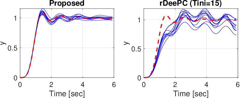
Refer to caption
Figure 3: Outputs of two-mass system with An=0.01A_{n}=0.01.
Table 4: Two-mass system: Comparison of MAE (Nd=1N_{d}=1)
DeePC DeePC rDeePC rDeePC D2PC
AnA_{n} (TiniT_{\rm ini}=4) (TiniT_{\rm ini}=15) (TiniT_{\rm ini}=4) (TiniT_{\rm ini}=15) (n¯=20\bar{n}=20)
10−810^{-8} <<0.001 <<0.001 0.397 0.093 <<0.001
10−410^{-4} 1.312 0.470 0.397 0.093 <<0.001
10−210^{-2} 0.993 1.523 0.486 0.092 0.009
10−110^{-1} 0.856 2.984 0.808 0.169 0.129

From Table 5, we again observe that MAE of D2PC tends to decrease as n¯\bar{n} is increased, and from Table 6, it is seen that MAE of D2PC tends to decrease with increasing NdN_{d}. We also applied the same averaging technique to DeePC, that is, the computation of UpU_{p}, UfU_{f}, YpY_{p}, and YfY_{f} are averaged over multiple data samples. As seen in Table 6, it was not effective (as briefly discussed in Section 4.3).

Table 5: Two-mass system: MAE of D2PC for various n¯\bar{n} (Nd=1N_{d}=1)
n¯\bar{n} 4 6 8 10 15 20
An=10−2A_{n}=10^{-2} 4.951 0.842 0.237 0.057 0.012 0.009
An=10−1A_{n}=10^{-1} 6.284 3.993 2.732 0.436 0.144 0.129
Table 6: Two-mass system (An=0.1A_{n}=0.1): MAE for various NdN_{d}
NdN_{d} 1 5 20 50 500
D2PC(n¯=20\bar{n}=20) 0.129 0.059 0.032 0.033 0.028
rDeePC(TiniT_{\rm ini}=15) 0.169 0.225 0.416 0.598 0.776

5.3 Four Tank System

Our last example is a multi-input-multi-output (MIMO) system. Consider a four tank system of Fig. 1.(c), whose discrete-time representation is given by Berberich et al. 2020:

A\displaystyle A =[0.92100.041000.91800.033000.92400000.937],B=[0.0170.0010.0010.02300.0610.0720]\displaystyle=\begin{bmatrix}0.921&0&0.041&0\\ 0&0.918&0&0.033\\ 0&0&0.924&0\\ 0&0&0&0.937\end{bmatrix},\ B=\begin{bmatrix}0.017&0.001\\ 0.001&0.023\\ 0&0.061\\ 0.072&0\end{bmatrix}
C\displaystyle C =[10000100].\displaystyle=\begin{bmatrix}1&0&0&0\\ 0&1&0&0\end{bmatrix}.

As in Berberich et al. 2020, the control goal is to make the output y⁡(t)y(t) track a setpoint r⁡(t)=[0.65, 0.77]Tr(t)=[0.65,\ 0.77]^{T}. Most of design parameters are chosen as the same as in Berberich et al. 2020: N=30N=30, Q=3​I2Q=3I_{2}, R=0.01​I2R=0.01I_{2}, and there are no input/output constraints. We also took the same parameters for rDeePC: λg=0.1\lambda_{g}=0.1, λy=1000\lambda_{y}=1000, and T=400T=400.

For actual plant, it is assumed that nothing is known but we assume that the order is less than n¯=30\bar{n}=30 (which is again far beyond the usual expectation of four tank system). Computer simulations are carried out and the results are summarized in Table 7. From Tables 8 and 9, we observe the same tendency as before for the MIMO system.

From the repeated simulation study, we found that a suitable choice of the regularization parameters for rDeePC is not trivial, but for D2PC, choosing two parameters n¯\bar{n} and NdN_{d} was relatively straightforward.

6 Conclusion

We have presented a new data-driven, output-feedback predictive control scheme for multi-input-multi-output, unknown, linear time-invariant plants. The order of the plant need not be known, which is in a sharp contrast to other popular methods such as (Lewis et al. 2012; Rizvi & Lin 2018; De Persis & Tesi 2019). There are only two tuning parameters n¯\bar{n} and NdN_{d} for the proposed controller, and it was demonstrated through three benchmark examples that increasing both parameters makes the closed-loop less sensitive to the measurement noise. Requiring relatively small length of episode data, it can be an effective method for unstable plants. If there is no input/output constraint in the optimization problem, the QP of D2PC is analytically solved and the optimal control becomes a linear feedback. Therefore, the proposed method can be considered as a constructive way to obtain a data-driven output-feedback LQR controller.

Table 7: Four tank system: Comparison of MAE (Nd=1N_{d}=1)
DeePC DeePC rDeePC rDeePC D2PC
AnA_{n} (TiniT_{\rm ini}=4) (TiniT_{\rm ini}=30) (TiniT_{\rm ini}=4) (TiniT_{\rm ini}=30) (n¯=30\bar{n}=30)
10−710^{-7} <<0.001 <<0.001 0.010 0.010 <<0.001
10−310^{-3} 0.952 0.939 0.013 0.010 0.001
10−210^{-2} 0.952 0.952 0.089 0.021 0.007
10−110^{-1} 0.952 0.952 0.515 0.200 0.074
Table 8: Four tank system: MAE of D2PC for various n¯\bar{n} (Nd=1N_{d}=1)
n¯\bar{n} 4 6 10 15 20 30
An=10−2A_{n}=10^{-2} 0.053 0.029 0.014 0.008 0.006 0.007
An=10−1A_{n}=10^{-1} 0.660 0.408 0.189 0.096 0.079 0.074
Table 9: Four tank system (An=0.1A_{n}=0.1): MAE for various NdN_{d}
NdN_{d} 1 5 20 50 500
D2PC(n¯=30\bar{n}=30) 0.074 0.033 0.020 0.015 0.013
rDeePC(Tini=30T_{\rm ini}=30) 0.200 0.122 0.124 0.184 0.418

References

  • Berberich et al. (2020) Berberich, J., Kohler, J., Muller, M., & Allgower, F. (2020). Data-driven model predictive control with stability and robustness guarantees. IEEE Trans. Automat. Contr.
  • Coulson et al. (2019) Coulson, J., Lygeros, J., & Dorfler, F. (2019). Data-enabled predictive control: In the shallows of the DeePC. In Proc. of European Control Conference.
  • De Persis & Tesi (2019) De Persis, C. & Tesi, P. (2019). Formulas for data-driven control: Stabilization, optimality, and robustness. IEEE Trans. Automat. Contr., 65, 909–924.
  • Elokda et al. (2019) Elokda, E., Coulson, J., Beuchat, P., Lygeros, J., & Dörfler, F. (2019). Data-enabled predictive control for quadcopters. (internal report of ETH)
  • Goodwin & Sin (2014) Goodwin, G. & Sin, K. (2014). Adaptive filtering prediction and control. Courier Corporation.
  • Lewis et al. (2012) Lewis, F.L., Vrabie, D., & Vamvoudakis, K.G. (2012). Reinforcement learning and feedback control: Using natural decision methods to design optimal adaptive controllers. IEEE Control Syst. Magazine, 32(6), 76–105.
  • Quanser Inc. (2008) Quanser Inc. (2008). Inverted pendulum user manuals.
  • Rizvi & Lin (2018) Rizvi, S.A.A. & Lin, Z. (2018). Output feedback Q-learning control for the discrete-time linear quadratic regulator problem. IEEE Trans. Neural Netw. Learn. Syst., 30(5), 1523–1536.
  • Stellato et al. (2020) Stellato, B., Banjac, G., Goulart, P., Bemporad, A., & Boyd, S. (2020). OSQP: an operator splitting solver for quadratic programs. Math. Program. Comput., 12, 637–672.
  • van Waarde et al. (2020) van Waarde, H. J., De Persis, C. D., Camlibel, M., & Tesi, P. (2020). Willems’ fundamental lemma for state-space systems and its extension to multiple datasets. IEEE Control Syst. Lett., 4, 602–607.
  • Wie & Bernstein (1992) Wie, B. & Bernstein, D. S. (1992). Benchmark problems for robust control design. In 1992 American Control Conference, pp. 2047–2048.
  • Willems et al. (2005) Willems, J., Rapisarda, P., Markovsky, I., & Moor, B. D. (2005). A note on persistency of excitation. Syst. Control. Lett., 54, 325–329.