Phase Boundary Segregation in Multicomponent Alloys: A Diffuse-Interface Thermodynamic Model

We invoke the concept of an interfacial phase or complexion for the interphase boundary (IB). That is, a compositionally-homogeneous layer of IB phase $i$ is governed by a fundamental thermodynamic equation distinct from that of the adjacent matrix $m$ and precipitate $p$ phases. This description follows from the classical treatment of solute segregation to free surfaces and grain boundaries (GB) (Cahn 1979; McLean 1957; Sutton and Balluffi 1995; Guttmann et al. 1979; Frolov and Mishin 2015), and the non-classical treatment of diffuse segregation to GBs in phase-field models (Cha et al. 2002; Kim and Park 2008; Abdeljawad and Foiles 2015; Abdeljawad et al. 2017; Kim et al. 2016).

A non-conserved phase field $\phi(\bm{x})$ variable is used to represent the phases: $m$ at $\phi=0$, $i$ at $\phi=0.5$, and $p$ at $\phi=1$. Any infinitesimal volume around the spatial location $\bm{x}$ is defined as a hypothetical thermodynamic mixture of $m$, $i$ and $p$ phases. The alloy is composed of the primary components $1$ and $2$, which act as solvents to from the two-phase system, and additional components $3,4,\ldots,\mathcal{N}$ which act as solutes. The mole fractions corresponding to a phase are represented by the phase concentration variables as $c_{\theta m}(\bm{x})$, $c_{\theta i}(\bm{x})$ and $c_{\theta p}(\bm{x})$; where, $\theta=1,2,3,\ldots,\mathcal{N}$.

We introduce interpolating functions $M(\phi)$, $I(\phi)$ and $P(\phi)$ for each of the phases $m$, $i$ and $p$. These functions serve as local phase fractions to define effective properties at $\bm{x}$ as a mixture of the phase properties. The effective concentrations $c_{\theta}(\bm{x})$ are defined by the mixture rule as

The local effective free energy density $f(\bm{c},\phi)$ is defined using the local phase-specific free energy densities $f^{\psi}(c_{2\psi},c_{3\psi},\ldots,c_{\mathcal{N}\psi})$ as

where $\bm{c}=\{c_{2},c_{3},\ldots,c_{\mathcal{N}}\}$. Under the assumption of substitutional solution and identical molar volumes of the components across the alloy, the effective concentrations satisfy $c_{1}(\bm{x})=1-\sum_{\theta=2:\mathcal{N}}c_{\theta}(\bm{x})$.

The phase concentrations $c_{\theta\psi}(\bm{x})$ at any given point are constrained by the condition of equal diffusion potential between the phases as

where ${\mu}_{\theta 1}\equiv\mu_{\theta}-\mu_{1}$ ($\theta=2:\mathcal{N}$) are the diffusion potentials. The above conditions follow from the KKS (Kim-Kim-Suzuki) phase-field formulation—originally developed for two-phase alloy solidification (Kim et al. 1999), later applied for GB segregation in two-grain alloy with GB phase (Cha et al. 2002; Kim and Park 2008; Kim et al. 2016), and recently developed for IB segregation in two-phase alloy with IB phase (Kadambi et al. 2020a; Kadambi et al. 2020b; Kadambi 2020).

The functional forms of the interpolating functions are chosen to satisfy the definition of exclusive phases as $M(\phi=0)=1$, $I(\phi=0.5)=1$ and $P(\phi=1)=1$, and the phase-mixture rule $M(\phi)+P(\phi)+I(\phi)=1$. For the sake of continuity in the derivatives, $M(\phi)$ and $P(\phi)$ $\in C^{1}[0,1]$ are chosen to be differentiable, piecewise functions. A convenient choice of interpolating functions constructed from the double-well form $I(\phi)=16\phi^{2}(1-\phi)^{2}$ is shown in Fig. 2. Note that for $\phi\in[0,0.5)$, $M(\phi)=1-I(\phi)$ and $P(\phi)=0$; for $\phi\in(0.5,1]$, $M(\phi)=0$ and $P(\phi)=1-I(\phi)$.

Given the local microstructure and its properties thus far, the overall free energy of the domain of volume $V$ can be defined by the functional,

where the second term in the integrand is the gradient energy density due to $\phi$, with $\varepsilon^{2}$ representing the gradient energy coefficient.

Following classical linear irreversible thermodynamics, the concentration fields evolve temporally under mass conservation as

where $\theta=2:\mathcal{N}$. The variational derivatives take the simplified definition as $\delta\mathcal{F}/\delta c_{\theta}=\partial f/\partial c_{\theta}={\mu}_{\theta 1}$. $\mathbf{\mathcal{M}}$ is the diffusion mobility matrix with components $\mathcal{M}_{\theta\xi}=\sum_{j=1:\mathcal{N}}(\delta_{k\xi j}-c_{\xi})(\delta_{j\theta}-c_{\theta})c_{j}\mathcal{M}_{j}$. $\mathcal{M}_{\theta}$ is the atomic mobility of component $\theta$ ($=1:\mathcal{N}$); $\mathcal{M}_{\theta}$ can be expressed in terms of the phase-dependent atomic mobilities as $\mathcal{M}_{\theta}=M(\phi)\mathcal{M}_{\theta}^{m}+I(\phi)\mathcal{M}_{\theta}^{i}+P(\phi)\mathcal{M}_{\theta}^{p}$.

Following Allen-Cahn dynamics, the non-conserved field $\phi$ evolves temporally as

where $\mathcal{L}$ is the kinetic mobility parameter for the interface.

We now consider a one-dimensional, planar IB at stationary equilibrium. The microstructure fields become invariant with time and will be denoted by $\phi_{e}(x)$ and $\bm{c}^{e}(x)$. Eqs. 5 and 6 reduce to

where $\mu_{\theta 1}^{e}$ are the equilibrium diffusion potentials. $\mu_{\theta 1}^{e}$ are constant across $x$ as required by the exchange of atoms between substitutional sites (Balluffi et al. 2005). The conditions (Eq. 3) for the equality of diffusion potentials at a point now read

The above relations imply that the phase-concentrations become spatially constant, i.e. $c_{\theta\psi}(x)=c_{\theta\psi}^{e}$. Therefore, the effective concentration fields (Eq. 1) are given by

Multiplying Eq. 8 with $d\phi_{e}/dx$ and integrating piecewise with respect to $x$ from $-\infty$ to $0$ and $0$ to $+\infty$ yields the following equilibrium relations between $m$, $i$ and $p$ (see Appendix A for derivation). Here, the limits of integration $-\infty$, $0$, and $+\infty$ refer to the far-field matrix, the exclusive IB and the far-field precipitate phases, respectively.

and

Eq. 9 and  12 constitute the well-known common tangent hyperplane condition for equilibrium between the bulk phase free energy hypersurfaces $f^{m}$ and $f^{p}$. Eq. II.2 and Eq. 9 constitute the parallel tangent hyperplane conditions for the equilibrium of the IB phase $f^{i}$ with respect to the bulk phases. For known convex functions of $f^{m}$, $f^{i}$ and $f^{p}$, the above conditions uniquely determine the equilibrium phase concentrations $c^{e}_{\theta\psi}$. $W_{e}$ represents the vertical distance between the two parallel tangent hyperplanes of $i$ and $m/p$. Physically, $W_{e}$ describes the free energy for the formation of a unit volume of equilibrium IB phase from the equilibrium matrix phase (or equivalently from the equilibrium precipitate phase) (Hillert 1975).

Substituting Eqs. 2 and II.2 in Eq. 8, we obtain the expression for the stationary phase-field profile $\phi_{e}(x)$ as (see Appendix A for derivation)

which can be integrated to obtain

The above expression depends only on the functional form of $I=16\phi^{2}(1-\phi)^{2}$. $W_{e}$ depends on the equilibrium phase concentrations, which are constants across the microstructure. Therefore, $W_{e}$ is a constant and the above expression can be readily integrated to obtain the well-known closed-form solution

The width $\lambda$ of the diffuse IB (defined by the bounds $\phi_{e}=0.1$ and $\phi_{e}=0.9$) is given by

We can now obtain expressions for the classical excess quantities from the equilibrium diffuse IB. The excess IB energy per unit IB area, $\gamma$, is the excess grand potential evaluated as (see Appendix B for derivation)

where $\pm l$ are locations within the bulk phases far-field of the interface. The integrand $2W_{e}I(\phi_{e}(x))\equiv\Omega(x)$ describes the energy density across the system in excess of the thermodynamic mixture of the equilibrium bulk phases. The integrand vanishes within the bulk phases since $I\left(\phi_{e}(\pm l)\right)\rightarrow 0$, and therefore, the integral converges. This property makes $\gamma$ an invariant thermodynamic quantity that is independent of the specific choice of the layer thickness (McFadden and Wheeler 2002).

The extensive solute excess quantities are evaluated by adapting Cahn’s layer approach (Cahn 1979) to the phase-field model (see Appendix C for derivations). The generalized Gibbs adsorption equation relating the change in $\gamma$ to the independent variations of intensive quantities, temperature $T$ and $\mu^{e}_{\theta}$, is obtained as (Cahn 1979; Frolov and Mishin 2015)

where $\Gamma^{(1,2)}_{S}$ is the relative entropy excess and $\Gamma^{(1,2)}_{\xi}$ is the relative solute excess for $\xi$, defined per unit interface area. The chemical potentials of the base components $1$ and $2$ have been eliminated with the aid of equilibrium conditions between the two bulk phases, and thus, $\Gamma^{(1,2)}_{1/2}=0$. The excess quantity $\Gamma^{(1,2)}_{S/\xi}$ describes the difference in the amount of entropy/component-$\theta$ between the chosen layer—containing the diffuse interface—and that of a hypothetical system. The hypothetical system is constructed from the two homogeneous bulk phases in such a proportion that the total amount of $1$ and $2$ is equal to that in the original layer (Cahn 1979; Frolov and Mishin 2015). Analytic expressions for these quantities were realized from the equilibrium phase and concentration fields as

where $\theta=1:\mathcal{N}$, $c^{e}_{1\psi}=1-\sum_{k=2:\mathcal{N}}c^{e}_{k\psi}$, and

$C^{xs}_{\xi}$ is the Gibbs solute excess evaluated from the effective concentration fields using the Gibbs dividing surface at $x=0$. Since the equilibrium concentrations are generally unequal in the two bulk phases, $C^{xs}_{\xi}$ depends on the specific location of the dividing surface within the diffuse IB. Note that $\Gamma^{(1,2)}_{\xi}$ is independent of the position of the dividing surface, and is an invariant thermodynamic quantity like $\gamma$. A similar expression is obtained for the $\Gamma^{(1,2)}_{S}$ (Eq. C).

The Gibbs adsorption isotherm can be written in terms of the derivatives of the matrix-phase concentrations $c^{e}_{\theta m}$ as

where $\mu^{e}_{\theta}=f^{m}_{e}+\sum_{k=2:\mathcal{N}}\left(\delta_{\theta k}-c^{e}_{km}\right)\mu^{e}_{k1}$ ($\delta_{\theta k}$ is the Kronecker delta) (Lupis 1983).

We assume regular solution behavior for the bulk and IB phases. The free energy density-composition dependence characteristic to $\psi$ is given by

Here, the energetics of $\theta$ in all the phases $\psi$ are defined from the same pure component reference state $\{\pi\theta\}$ (DeHoff 2006). The reference states can have crystal structures distinct from that of the solid-solution $\psi$. $G^{\psi}_{\theta}\{\pi\theta\}$ accounts for the pure component energy of $\theta$ in $\psi$ with reference to ${\pi\theta}$. For mixing (second term), the structure of each component must be identical to that of the final solid-solution $\psi$. $L^{\psi}_{\theta\xi}\{\psi\theta,\psi\xi\}$ accounts for the non-ideal interaction energy between distinct components $\theta$ and $\xi$ in $\psi$, with reference to the pure components in $\psi$. Therefore, the parameters $G^{\psi}_{\theta}$ and $L^{\psi}_{\theta\xi}$ account for the distinct chemical and structural energetics of the bulk and interfacial phases. The final term in the equation is the ideal configurational entropy for mixing and $v_{m}$ is the molar volume.

Using Eq. II.4, the equilibrium compositions in the bulk phases are established by Eqs. 9 and  12. These constitute $\mathcal{N}$ equations in $2\left(\mathcal{N}-1\right)$ bulk-phase concentrations and allow $\mathcal{N}-2$ compositional degrees of freedom. We choose the matrix-phase solute concentrations $c^{e}_{3m},\ldots,c^{e}_{\mathcal{N}m}$ as the control variables, while the rest are to be uniquely determined.

The equilibrium composition in the IB phase $\psi=i$ is then established using Eq. II.4 in $\partial f^{i}/\partial c^{e}_{\theta i}=\partial f^{m}/\partial c^{e}_{\theta m}$ of Eq. 9. These constitute $\mathcal{N}-1$ segregation equations relating $\mathcal{N}-1$ unknowns $(c^{e}_{2i},\ldots,c^{e}_{\mathcal{N}i})$ to the known $(c^{e}_{2m},\ldots,c^{e}_{\mathcal{N}m})$. They can be written as

where

$\Delta E^{\theta 1}_{\text{seg}}$ describes the segregation energy resulting form the exchange of $\theta$ in $m$ with component $1$ in $i$. The above coupled and non-linear equations must be solved simultaneously to determine the equilibrium IB phase composition.

The segregation equations obtained in our model are equivalent to the generalized multicomponent grain boundary segregation isotherms of Guttmann (Guttmann 1975). For an ideal alloy ($L=0$), the equations reduce to the decoupled multicomponent versions of Langmuir-McLean (McLean 1957; Lejček 2010). For a non-ideal ($L\neq 0$) alloy, the second term in Eq. 24 is identical to that of the Fowler-Guggenheim isotherm (Guggenheim 1985; Lejček 2010) representing the interaction between $\theta$ and $1$. The third and following terms are the cross terms relating segregation of $\theta$ with segregation of $\xi$. For IB segregation, these interactions become important for a quaternary (or higher-order) alloy as shown in the next section.

In this section, we apply the phase-field model to explore segregation behavior in quaternary alloys. The model is non-dimensionalized by setting $x=l_{o}\tilde{x}$, $t=t_{o}\tilde{t}$, $T=T_{o}\tilde{T}$ and $f^{\psi}=\left(RT_{o}/v_{m}\right)\tilde{f}^{\psi}$ ($\psi=m,i,p$). $l_{o}$, $t_{o}$ and $T_{o}$ are the characteristic length, time and temperature, respectively, and $RT_{o}/v_{m}$ is the characteristic energy. The dimensionless quantities are denoted by the tilde symbol. The free energy density for a quaternary alloy now takes the form, $\tilde{f}^{\psi}=\tilde{G}^{\psi}_{1}c_{1\psi}+\tilde{G}^{\psi}_{2}c_{2\psi}+\tilde{G}^{\psi}_{3}c_{3\psi}+\tilde{G}^{\psi}_{4}c_{4\psi}+\tilde{L}^{\psi}_{12}c_{1\psi}c_{2\psi}+\tilde{L}^{\psi}_{13}c_{1\psi}c_{3\psi}+\tilde{L}^{\psi}_{23}c_{2\psi}c_{3\psi}+\tilde{L}^{\psi}_{14}c_{1\psi}c_{4\psi}+\tilde{L}^{\psi}_{24}c_{2\psi}c_{4\psi}+\tilde{L}^{\psi}_{34}c_{3\psi}c_{4\psi}+\tilde{T}\left(c_{1\psi}\ln{c_{1\psi}}+c_{2\psi}\ln{c_{2\psi}}+c_{3\psi}\ln{c_{3\psi}}+c_{4\psi}\ln{c_{4\psi}}\right)$. The equilibrium equations in Sec. II.1 are replaced with the dimensionless parameters: $\tilde{\varepsilon}^{2}=\varepsilon^{2}/\left[l_{o}^{2}\left(RT_{o}/v_{m}\right)\right]$ and $\tilde{\mu}^{e}=\mu^{e}/\left(RT_{o}/v_{m}\right)$.

For the parametric study of the model, we assume $(\tilde{\varepsilon}^{2},\tilde{T})=(1,1)$. The dimensionless results can be dimensionalized as $\gamma=\left(RT_{o}l_{o}/v_{m}\right)\tilde{\gamma}$ and $\Gamma_{\xi}^{(1,2)}=(l_{o}/v_{m})\tilde{\Gamma}_{\xi}^{(1,2)}$. For example, setting the characteristic scales to be $l_{o}=1$ nm, $T_{o}=300$ K and $v_{m}=7\times 10^{-6}$ m³/mol yields $\gamma=0.36\tilde{\gamma}$ J/m² and $\Gamma_{\xi}^{(1,2)}=\left(1.43\times 10^{-4}\right)\tilde{\Gamma}_{\xi}^{(1,2)}$ mol/m².

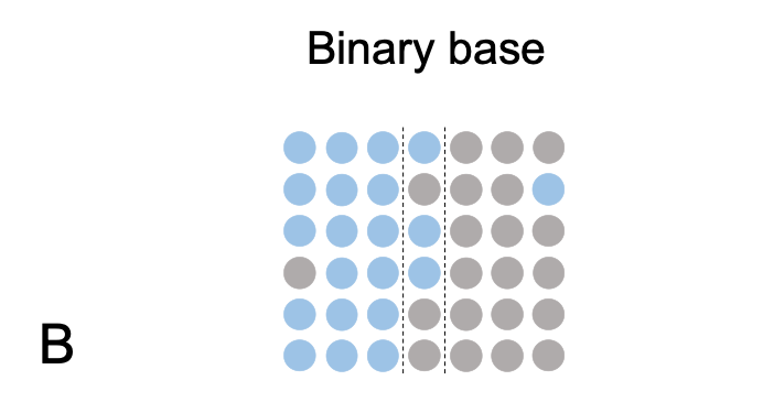
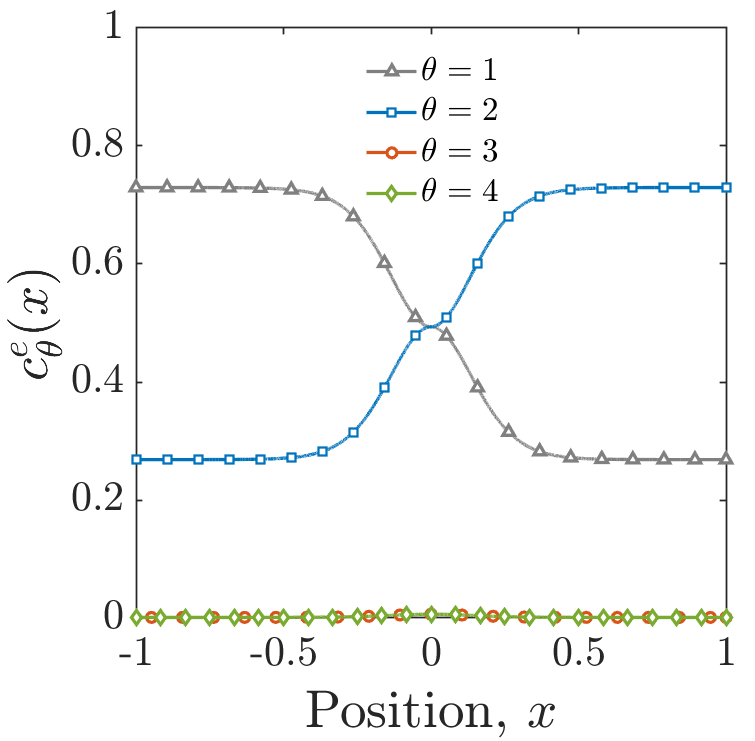
We choose an ideal binary base alloy ($1$-$2$) that forms a two-phase coexistence region in the bulk phase diagram (see Table 1 and Ref. (Kadambi et al. 2020a)). The alloy microstructure and the equilibrium concentration profiles are shown in Fig. 3 and represented by the schematic with the label B. The matrix phase $m$ is rich in $1$ ($c^{e}_{2m}\approx 0.27$) while the precipitate phase $p$ is rich in $2$ ($c^{e}_{2p}\approx 0.73$). The IB phase $i$ has been chosen to have an equilibrium concentration as the average of $m$ and $p$ phases ($c^{e}_{2m}\approx 0.5$). The phase-field calculations yield a relative excess entropy of $\tilde{\Gamma}^{(1,2)}_{S}=0$ and an excess IB energy of $\tilde{\gamma}_{B}=1.2$ units.

Next we consider the addition of solutes $3$ and $4$ individually to form the ternaries ($1$-$2$)-$\xi$ ($\xi=3/4$). Two types of solute behaviors are considered as references–ternary non-segregating (TN) and ternary segregating (TS). The alloy microstructures of TN and TS are shown via representative schematics and equilibrium concentration profiles in Fig. 3. TN alloys are realized for $L^{i}_{\theta\xi}$ = $L^{m/p}_{\theta\xi}$ ($\theta=1,2$), i.e. when the regular solution interactions are identical or ideal across all phases in the alloy. For these cases, $\tilde{G}^{i}_{\theta}\approx 1.62$ units was derived from Eq. 23 such that $c^{e}_{\xi i}=c^{e}_{\xi{m/p}}$ is satisfied. Calculations of excess quantities yields $\tilde{\Gamma}^{(1,2)}_{\xi}=0$ and $\tilde{\gamma}=\tilde{\gamma}_{B}$. TS alloys, on the other hand, are realized for $L^{i}_{\theta\xi}<L^{m/p}_{\theta\xi}$, i.e. when the solute $\xi$ interacts more favorably with $\theta$ in $i$. These can further be noted for the ternary parameters $L^{i}_{\theta\xi}$ and $L^{m/p}_{\theta\xi}$ listed in Table 2. Calculation of excess quantities yield a positive segregation $\tilde{\Gamma}^{(1,2)}_{\xi}>0$ and a reduced IB energy $\tilde{\gamma}<\tilde{\gamma}_{\text{B}}$. For simplicity, we omit segregation cases arising from variations in the pure energies $\tilde{G}^{\psi}_{\xi}$. We also simplify the parameter space by considering that the solutes interact identically within the bulk phases $m$ and $p$, and with solvent component $1$ and $2$. This condition is captured in Table 2 by $L^{m/p}_{\theta 3}$ and $L^{m/p}_{\theta 4}$, and lead to vanishing cross terms between the solute and solvent in Eq. 24, $\tilde{L}^{\psi}_{12}+\tilde{L}^{\psi}_{1\xi}-\tilde{L}^{\psi}_{2\xi}=0$.

For the sake of completeness, we note here that the variation of excess quantities for the ternaries can be read from the limits $c^{e}_{\xi m}\rightarrow 0$ of $\tilde{\Gamma}^{(1,2)}_{\xi}$ and $\tilde{\gamma}$ contour plots presented for quaternary alloys in Fig. 7. As the matrix-phase concentration $c^{e}_{\xi m}$ is increased, TN alloys (in I–III) exhibit constant values of $\tilde{\Gamma}^{(1,2)}_{\xi}=0$ and $\tilde{\gamma}=\tilde{\gamma}_{\text{B}}$. TS alloys (in V–VIII) exhibit a positive and increasing $\tilde{\Gamma}^{(1,2)}_{\xi}$, with a correspondingly decreasing $\tilde{\gamma}$ from that of $\tilde{\gamma}_{\text{B}}$. The model parameters used for the reference alloys here were inspired by our earlier works on phase boundary segregation in binary (Kadambi et al. 2020a) and ternary (Kadambi et al. 2020b) systems. Kadambi et al. 2020b rigorously demonstrated the validity of the current phase-field approach with the Gibbs adsorption isotherm $d\tilde{\gamma}=-\tilde{\Gamma}^{(1,2)}_{\xi}d\mu^{e}_{\xi}$.

In the case studies presented below, we examine the effect of combined solute addition in the quaternary ($1$-$2$)-$3$-$4$ alloy. The interaction between solutes governed by $\tilde{L}^{m/p}_{34}$ and $\tilde{L}^{i}_{34}$ forms the basis for understanding the segregation behavior in ($1$-$2$)-$3$-$4$ relative to ($1$-$2$)-$3$ (TN or TS) and ($1$-$2$)-$4$ (TN or TS). The different cases examined here are labeled I through IX in Table 2.

We can understand the interfacial properties of the diffuse-interface formulation (Sec. II) by first considering the interface to be a GB in a two-component, single-phase alloy. $\phi(x)$ now denotes the variation in crystallographic orientation across the diffuse GB. The bulk-phase free energies, phase concentrations and local phase fractions take the following simplified forms: $f^{p}\equiv f^{m}$, $c_{\theta p}\equiv c_{\theta m}$ and $P(\phi)\equiv M(\phi)=1-I(\phi)$ for $\phi\in[0,1]$. Therefore, the local free energy density (Eq. 2) becomes $f(c_{2},\phi)=f^{m}(c_{2m})[1-I(\phi)]+f^{i}(c_{2i})I(\phi)$. This reduced model is equivalent in most aspects to existing phase-field formulations (Cha et al. 2002; Abdeljawad and Foiles 2015; Kim et al. 2016) for GB segregation. Invoking the regular solution behavior, and imposing the limit of pure component $1$, we get $f(\phi)=G^{m}_{1}+(G^{i}_{1}-G^{m}_{1})I(\phi)$. The term $(G^{i}_{1}-G^{m}_{1})I(\phi)$ is analogous to the classical, symmetric double-well potential $W_{\phi}I(\phi)$ used in standard phase-field models for grain growth, alloy solidification and antiphase boundary motion (Provatas and Elder 2011). Since the pure component energies $G^{\psi}_{1}\{\pi 1\}$ are defined from the same pure component reference state $\pi 1$ (Sec. II.4), $G^{i}_{1}-G^{m}_{1}>0$ accounts for the excess structural energy of the GB phase over that of the matrix. The GB energy $\gamma$ of this pure metal is given by $\gamma_{1}\approx 0.943\varepsilon\sqrt{G^{i}_{1}-G^{m}_{1}}$ (Eq. 17). However, for a multicomponent alloy, the equilibrium between the GB phase and the bulk matrix phase is established by the parallel tangent construction, which determines the equilibrium GB phase concentrations $\textbf{c}^{e}_{i}$ and parallel tangent distance $W_{e}(\textbf{c}^{e}_{i},\textbf{c}^{e}_{m})$. $W_{e}$ then represents the free energy for formation of a unit volume of the equilibrium GB phase from the equilibrium bulk phase, and therefore, captures not only the the structural energetics but also the compositional dependence (Hillert 1975). Therefore, the GB energy for a multicomponent alloy can be obtained (from Eqs. 12 and 17) by setting $p\equiv m$, giving $\gamma\approx 0.943\varepsilon\sqrt{W_{e}(\textbf{c}^{e}_{i},\textbf{c}^{e}_{m})}$.

Now consider the interface to be the IB in a two-phase alloy, i.e. $p\not\equiv m$. The local free energy density $f(\textbf{c}^{e},\phi_{e})$ (Eq. 2) will take the form of an asymmetric double-well potential as shown below. Reducing the system to the theoretical limit of a pure component $1$, we get $f(\phi)=G^{m}_{1}+(G^{i}_{1}-G^{m}_{1})I(\phi)$ for $\phi\leq 0.5$ and $f(\phi)=G^{p}_{1}+(G^{i}_{1}-G^{p}_{1})I(\phi)$ for $\phi>0.5$. In conventional phase-field formulations for two structurally-distinct phases, a symmetric double-well potential $W_{\phi}I(\phi)$ is employed to define the excess structural energy across the diffuse IB. In the current formulation, the symmetric part is inherent in the second term $(G^{i}_{1}-G^{p}_{1})I(\phi)$ of the piecewise function, while the first terms $G^{m}_{1}\neq G^{p}_{1}$ results in the asymmetry. For a multicomponent alloy, the model additionally captures the compositional dependence: for an equilibrium, planar IB, $f(\textbf{c}^{e},\phi_{e})=f^{m}(\textbf{c}^{e})+W_{e}(\textbf{c}^{e})I(\phi)$ for $\phi_{e}\leq 0.5$ and $f(\textbf{c}^{e},\phi_{e})=f^{p}(\textbf{c}^{e})+W_{e}(\textbf{c}^{e})I(\phi_{e})$ for $\phi_{e}>0.5$; where $W_{e}(\textbf{c}^{e})\equiv f^{i}(\textbf{c}^{e})-f^{m}(\textbf{c}^{e})=f^{i}(\textbf{c}^{e})-f^{p}(\textbf{c}^{e})$. Therefore, analogous to the GB energy discussed in the preceding paragraph, the IB energy is obtained as $\gamma\approx 0.943\varepsilon\sqrt{W_{e}(\textbf{c}^{e}_{i},\textbf{c}^{e}_{m})}$. Thereby $\gamma$ accounts for the structural and the chemical energetics for the formation of the interfacial phase (via $W_{e}$) and the associated diffuse regions (via $\varepsilon$). The parametric study (Sec. III) showed the possibility of realizing $\gamma\rightarrow 0$ for synergistic, induced and enhanced co-segregation cases of quaternary alloys. However, the gradient energy contribution of the diffuse interface—together with the condition of equi-partitioning of the local excess grand-potential (Eq. A33)—imposes a theoretical restriction of $\gamma>0$, via $W_{e}>0$ in Eq. 17.

The regular solution assumption (Sec. II.4) for the bulk and IB phase thermodynamics allowed a variety of segregation/de-segregation behaviors to be realized. Parameterization was readily possible based on the physical significance afforded by regular solution thermodynamic parameters. Compared to IBs, multicomponent segregation in GBs have been well studied, both experimentally and theoretically (Guttmann and McLean 1979; Erhart and Grabke 1981; Guttmann et al. 1982; Lejček 2010; Lejček 2013; Xing et al. 2018; Xing et al. 2019). IB segregation in quaternary, two-phase alloys can be found to be similar in many aspects to GB segregation in ternary, single-phase alloys. For example, the addition of certain secondary solutes is well known to enhance GB segregation of the primary solute due to mutually attractive interaction between the solutes at the GB (Gas et al. 1982). This is analogous to case VI. Another example is the addition of a secondary solute which is also known to mitigate GB embrittlement caused by the undesired segregation of the primary solute–i.e. the solutes compete for GB sites and the strongly-segregating solute preferentially segregates by desegregating the weaker solute (Suzuki et al. 1991). This is analogous to case VII. Therefore, based on the nature of mutual interaction between the solutes, their combined addition in the ternaries causes GB segregation behaviors that are fundamentally different from that of the individual solutes in their respective binaries. Xing et al. (Xing et al. 2018) presented a classification of the GB segregation/de-segregation behaviors in ternary single-phase alloys. The segregation mechanisms observed in current study are analogous to those observed for GBs.

The case studies presented in Sec. III are qualitatively representative of the observed mechanisms in the literature. As mentioned in Sec. I, numerous cases of IB co-segregation has already been reported. Several experimental and first-principles studies demonstrate enhanced high-temperature stability of the quaternary alloys due to IB co-segregation and its associated reduction in IB energy $\gamma$. Moreover, some studies suggest the need to desegregate certain solute from the IB: for example, Si at Al(matrix)/$\theta^{\prime}$-Al₂Cu in (Al-Cu)-Mn-Zr-Si is found to be deleterious to the microstructural stability in larger amounts (Shyam et al. 2019); Ca at Mg(matrix)/Al₁₁La₃ in (Mg-Al)-La-Ca-Mn is found to destabilize the strengthening precipitate (Yang et al. 2020) by by nucleating Al₂Ca. Therefore, it is also necessary to understand the de-segregation mechanisms (cases VII and VIII) so that alloys could be designed to favor beneficial solutes to segregate in preference to the undesired impurities.

The diffuse-interface thermodynamic formulation was shown to be consistent (see Sec. C) with the classical Gibbs interface phase rule (Frolov and Mishin 2015). At a given temperature, the number of components ($n_{\mathcal{N}}$) and the number of coexisting bulk phases ($n_{\psi}$) dictates the number of compositional degrees of freedom ($d_{\theta}^{f}=n_{\mathcal{N}}-n_{\psi}$). Thereby, two compositional degrees of freedom in solute $3$ and $4$ concentrations were available to modulate the properties of the quaternary IB in Sec. III. Analogously, if the model is applied to a ternary GB (where the common tangent constraint between phases is removed), two compositional degrees of freedom in solutes $2$ and $3$ will be available. Therefore, in addition to multicomponent IB segregation, the current approach has the potential to be employed for recently observed GB segregations in multi-principal element/high entropy alloys (Li et al. 2020).

References

- Roy et al. (2017) S. Roy, L. F. Allard, A. Rodriguez, W. D. Porter, and A. Shyam, Comparative evaluation of cast aluminum alloys for automotive cylinder heads: Part II—mechanical and thermal properties, Metallurgical and Materials Transactions A 48, 2543 (2017).
- Mendis et al. (2006) C. Mendis, C. Bettles, M. Gibson, and C. Hutchinson, An enhanced age hardening response in Mg–Sn based alloys containing Zn, Materials Science and Engineering: A 435, 163 (2006).
- Seidman et al. (2002) D. N. Seidman, E. A. Marquis, and D. C. Dunand, Precipitation strengthening at ambient and elevated temperatures of heat-treatable Al(Sc) alloys, Acta Materialia 50, 4021 (2002).
- Pollock and Tin (2006) T. M. Pollock and S. Tin, Nickel-based superalloys for advanced turbine engines: chemistry, microstructure and properties, Journal of propulsion and power 22, 361 (2006).
- Bauer et al. (2012) A. Bauer, S. Neumeier, F. Pyczak, R. F. Singer, and M. Göken, Creep properties of different -strengthened Co-base superalloys, Materials Science and Engineering: A 550, 333 (2012).
- Zhao et al. (2018) Y. Zhao, H. Chen, Z. Lu, and T. Nieh, Thermal stability and coarsening of coherent particles in a precipitation-hardened (NiCoFeCr)94Ti2Al4 high-entropy alloy, Acta Materialia 147, 184 (2018).
- Gao et al. (2020) Y. Gao, P. Guan, R. Su, H. Chen, C. Yang, C. He, L. Cao, H. Song, J. Zhang, X. Zhang, et al., Segregation-sandwiched stable interface suffocates nanoprecipitate coarsening to elevate creep resistance, Materials Research Letters 8, 446 (2020).
- Ratke and Voorhees (2013) L. Ratke and P. W. Voorhees, Growth and Coarsening: Ostwald Ripening in Material Processing (Springer Science & Business Media, 2013).
- Clouet et al. (2006) E. Clouet, L. Laé, T. Épicier, W. Lefebvre, M. Nastar, and A. Deschamps, Complex precipitation pathways in multicomponent alloys, Nature Materials 5, 482 (2006).
- Marquis and Seidman (2005) E. A. Marquis and D. N. Seidman, Coarsening kinetics of nanoscale Al3Sc precipitates in an Al–Mg–Sc alloy, Acta Materialia 53, 4259 (2005).
- Cahn (1979) J. W. Cahn, Thermodynamics of solid and fluid surfaces, in Interfacial Segregation, edited by W. C. Johnson and J. M. Blakely (ASM, Metals Park, OH, 1979) pp. 3–23.
- Kaplan et al. (2013) W. D. Kaplan, D. Chatain, P. Wynblatt, and W. C. Carter, A review of wetting versus adsorption, complexions, and related phenomena: the rosetta stone of wetting, Journal of Materials Science 48, 5681 (2013).
- Frolov and Mishin (2015) T. Frolov and Y. Mishin, Phases, phase equilibria, and phase rules in low-dimensional systems, The Journal of Chemical Physics 143, 044706 (2015).
- Marquis et al. (2006) E. A. Marquis, D. N. Seidman, M. Asta, and C. Woodward, Composition evolution of nanoscale Al3Sc precipitates in an Al–Mg–Sc alloy: Experiments and computations, Acta Materialia 54, 119 (2006).
- Amouyal et al. (2008) Y. Amouyal, Z. Mao, and D. N. Seidman, Segregation of tungsten at (L12)/ (fcc) interfaces in a Ni-based superalloy: An atom-probe tomographic and first-principles study, Applied Physics Letters 93, 201905 (2008).
- Biswas et al. (2011) A. Biswas, D. J. Siegel, C. Wolverton, and D. N. Seidman, Precipitates in Al–Cu alloys revisited: Atom-probe tomographic experiments and first-principles calculations of compositional evolution and interfacial segregation, Acta Materialia 59, 6187 (2011).
- Shin et al. (2017) D. Shin, A. Shyam, S. Lee, Y. Yamamoto, and J. A. Haynes, Solute segregation at the Al/-Al2Cu interface in Al-Cu alloys, Acta Materialia 141, 327 (2017).
- Samolyuk et al. (2020) G. D. Samolyuk, M. Eisenbach, D. Shin, Y. N. Osetsky, A. Shyam, and J. R. Morris, Equilibrium solute segregation to matrix- precipitate interfaces in Al-Cu alloys from first principles, Phys. Rev. Materials 4, 073801 (2020).
- Hutchinson et al. (2001) C. R. Hutchinson, X. Fan, S. J. Pennycook, and G. J. Shiflet, On the origin of the high coarsening resistance of plates in Al–Cu–Mg–Ag alloys, Acta Materialia 49, 2827 (2001).
- Sun et al. (2009) L. Sun, D. L. Irving, M. A. Zikry, and D. Brenner, First-principles investigation of the structure and synergistic chemical bonding of Ag and Mg at the Al— interface in a Al–Cu–Mg–Ag alloy, Acta Materialia 57, 3522 (2009).
- Rosalie and Bourgeois (2012) J. M. Rosalie and L. Bourgeois, Silver segregation to (Al2Cu)–Al interfaces in Al–Cu–Ag alloys, Acta Materialia 60, 6033 (2012).
- Kang et al. (2014) S. J. Kang, Y.-W. Kim, M. Kim, and J.-M. Zuo, Determination of interfacial atomic structure, misfits and energetics of phase in Al–Cu–Mg–Ag alloy, Acta Materialia 81, 501 (2014).
- Biswas et al. (2010) A. Biswas, D. J. Siegel, and D. N. Seidman, Simultaneous segregation at coherent and semicoherent heterophase interfaces, Physical Review Letters 105, 076102 (2010).
- Shyam et al. (2019) A. Shyam, S. Roy, D. Shin, J. D. Poplawsky, L. Allard, Y. Yamamoto, J. Morris, B. Mazumder, J. Idrobo, A. Rodriguez, et al., Elevated temperature microstructural stability in cast alcumnzr alloys through solute segregation, Materials Science and Engineering: A 765, 138279 (2019).
- Wang and Wang (2008) Y.-J. Wang and C.-Y. Wang, The alloying mechanisms of Re, Ru in the quaternary Ni-based superalloys / interface: a first principles calculation, Materials Science and Engineering: A 490, 242 (2008).
- Wu et al. (2020) X. Wu, S. K. Makineni, C. H. Liebscher, G. Dehm, J. R. Mianroodi, P. Shanthraj, B. Svendsen, D. Bürger, G. Eggeler, D. Raabe, et al., Unveiling the re effect in ni-based single crystal superalloys, Nature communications 11, 1 (2020).
- Blum et al. (2020) I. Blum, S.-I. Baik, M. G. Kanatzidis, and D. N. Seidman, An integral method for the calculation of the reduction in interfacial free energy due to interfacial segregation, arXiv preprint arXiv:2003.01246 (2020).
- McLean (1957) D. McLean, Grain Boundaries in Metals (Oxford University Press, Oxford, 1957).
- Sutton and Balluffi (1995) A. P. Sutton and R. W. Balluffi, Interfaces in Crystalline Materials (Clarendon Press, 1995).
- Guttmann et al. (1979) M. Guttmann, D. McLean, W. Johnson, and J. Blakely, Interfacial segregation, ASM, Metals Park, Ohio 261 (1979).
- Cha et al. (2002) P.-R. Cha, S. G. Kim, D.-H. Yeon, and J.-K. Yoon, A phase field model for the solute drag on moving grain boundaries, Acta Materialia 50, 3817 (2002).
- Kim and Park (2008) S. G. Kim and Y. B. Park, Grain boundary segregation, solute drag and abnormal grain growth, Acta Materialia 56, 3739 (2008).
- Abdeljawad and Foiles (2015) F. Abdeljawad and S. M. Foiles, Stabilization of nanocrystalline alloys via grain boundary segregation: a diffuse interface model, Acta Materialia 101, 159 (2015).
- Abdeljawad et al. (2017) F. Abdeljawad, P. Lu, N. Argibay, B. G. Clark, B. L. Boyce, and S. M. Foiles, Grain boundary segregation in immiscible nanocrystalline alloys, Acta Materialia 126, 528 (2017).
- Kim et al. (2016) S. G. Kim, J. S. Lee, and B.-J. Lee, Thermodynamic properties of phase-field models for grain boundary segregation, Acta Materialia 112, 150 (2016).
- Kim et al. (1999) S. G. Kim, W. T. Kim, and T. Suzuki, Phase-field model for binary alloys, Physical Review E 60, 7186 (1999).
- Kadambi et al. (2020a) S. B. Kadambi, F. Abdeljawad, and S. Patala, A phase-field approach for modeling equilibrium solute segregation at the interphase boundary in binary alloys, Computational Materials Science 175, 109533 (2020a).
- Kadambi et al. (2020b) S. B. Kadambi, F. Abdeljawad, and S. Patala, Interphase boundary segregation and precipitate coarsening resistance in ternary alloys: An analytic phase-field model describing chemical effects, Acta Materialia 197, 283 (2020b).
- Kadambi (2020) S. B. Kadambi, Interphase Boundary Segregation Engineering (North Carolina State University, 2020).
- Balluffi et al. (2005) R. W. Balluffi, S. Allen, and W. C. Carter, Kinetics of Materials (John Wiley & Sons, 2005).
- Hillert (1975) M. Hillert, The uses of Gibbs free energy-composition diagrams, in Lectures on the Theory of Phase Transformations, edited by H. I. Aaronson (AIME, New York, 1975) Chap. 1, pp. 1–50.
- McFadden and Wheeler (2002) G. B. McFadden and A. Wheeler, On the Gibbs adsorption equation and diffuse interface models, in Proceedings of the Royal Society of London A: Mathematical, Physical and Engineering Sciences, Vol. 458 (The Royal Society, 2002) pp. 1129–1149.
- Lupis (1983) C. H. Lupis, Chemical Thermodynamics of Materials (North-Holland, New York, 1983).
- DeHoff (2006) R. DeHoff, Thermodynamics in Materials Science (CRC Press, 2006).
- Guttmann (1975) M. Guttmann, Equilibrium segregation in a ternary solution: A model for temper embrittlement, Surface Science 53, 213 (1975).
- Lejček (2010) P. Lejček, Grain Boundary Segregation in Metals, Vol. 136 (Springer Science & Business Media, 2010).
- Guggenheim (1985) E. A. Guggenheim, Thermodynamics. An Advanced Treatment for Chemists and Physicists (North-Holland, Amsterdam, 1985).
- Provatas and Elder (2011) N. Provatas and K. Elder, Phase-field Methods in Materials Science and Engineering (John Wiley & Sons, 2011).
- Guttmann and McLean (1979) M. Guttmann and D. McLean, Grain boundary segregation in multicomponent systems, Interfacial segregation , 261 (1979).
- Erhart and Grabke (1981) H. Erhart and H.-J. Grabke, Equilibrium segregation of phosphorus at grain boundaries of Fe–P, Fe–C–P, Fe–Cr–P, and Fe–Cr–C–P alloys, Metal Science 15, 401 (1981).
- Guttmann et al. (1982) M. Guttmann, P. Dumoulin, and M. Wayman, The thermodynamics of interactive co-segregation of phosphorus and alloying elements in iron and temper-brittle steels, Metallurgical Transactions A 13, 1693 (1982).
- Lejček (2013) P. Lejček, Effect of ternary solute interaction on interfacial segregation and grain boundary embrittlement, Journal of Materials Science 48, 4965 (2013).
- Xing et al. (2018) W. Xing, A. R. Kalidindi, D. Amram, and C. A. Schuh, Solute interaction effects on grain boundary segregation in ternary alloys, Acta Materialia 161, 285 (2018).
- Xing et al. (2019) W. Xing, S. A. Kube, A. R. Kalidindi, D. Amram, J. Schroers, and C. A. Schuh, Stability of ternary nanocrystalline alloys in the Pt–Pd–Au system, Materialia 8, 100449 (2019).
- Gas et al. (1982) P. Gas, M. Guttmann, and J. Bernardini, The interactive co-segregation of Sb and Ni at the grain boundaries of ultra-high purity Fe-base alloys, Acta Metallurgica 30, 1309 (1982).
- Suzuki et al. (1991) S. Suzuki, S. Tanii, K. Abiko, and H. Kimura, Site competition between sulfur and carbon at grain boundaries and their effects on the grain boundary cohesion in iron, Metallurgical Transactions A 18, 1109 (1991).
- Yang et al. (2020) Q. Yang, S. Lv, P. Qin, F. Meng, X. Qiu, X. Hua, K. Guan, W. Sun, X. Liu, and J. Meng, Interphase boundary segregation induced phase transformation in a high-pressure die casting Mg-Al-La-Ca-Mn alloy, Materials & Design , 108566 (2020).
- Li et al. (2020) L. Li, R. D. Kamachali, Z. Li, and Z. Zhang, Grain boundary energy effect on grain boundary segregation in an equiatomic high-entropy alloy, Physical Review Materials 4, 053603 (2020).
- Patala (2019) S. Patala, Understanding grain boundaries–the role of crystallography, structural descriptors and machine learning, Computational Materials Science 162, 281 (2019).
- Homer et al. (2015) E. R. Homer, S. Patala, and J. L. Priedeman, Grain boundary plane orientation fundamental zones and structure-property relationships, Scientific reports 5, 1 (2015).
- Banadaki et al. (2018) A. D. Banadaki, M. A. Tschopp, and S. Patala, An efficient monte carlo algorithm for determining the minimum energy structures of metallic grain boundaries, Computational Materials Science 155, 466 (2018).
- Zhang et al. (2016) W.-Z. Zhang, X.-F. Gu, and F.-Z. Dai, Faceted interfaces: a key feature to quantitative understanding of transformation morphology, npj Computational Materials 2, 1 (2016).
- Heo et al. (2011) T. W. Heo, S. Bhattacharyya, and L.-Q. Chen, A phase field study of strain energy effects on solute–grain boundary interactions, Acta materialia 59, 7800 (2011).
- Wheeler et al. (1993) A. A. Wheeler, W. J. Boettinger, and G. B. McFadden, Phase-field model of solute trapping during solidification, Physical Review E 47, 1893 (1993).
- Wheeler et al. (1992) A. A. Wheeler, W. J. Boettinger, and G. B. McFadden, Phase-field model for isothermal phase transitions in binary alloys, Physical Review A 45, 7424 (1992).