On quasinormal modes in 4D black hole solutions in the model
with anisotropic fluid
S. V. Bolokhov11 1 bol-rgs@yandex.ru,a and V. D. Ivashchuk22 2 ivashchuk@mail.ru,a,b
(a)
Institute of Gravitation and Cosmology,
Peoples’ Friendship University of Russia
(RUDN University),
6 Miklukho-Maklaya Street,
Moscow, 117198, Russian Federation
(b) Center for Gravitation and Fundamental Metrology,
VNIIMS, 46 Ozyornaya St., Moscow 119361, Russian Federation
Abstract
We consider a family of 4-dimensional black hole solutions from Dehnen et al. ( Grav. Cosmol. 9:153, arXiv: gr-qc/0211049, 2003) governed by natural number , which appear in the model with anisotropic fluid and the equations of state: , , where and are pressures in radial and transverse directions, respectively, and is the density. These equations of state obey weak, strong and dominant energy conditions. For the metric of the solution coincides with that of the Reissner-Nordström one. The global structure of solutions is outlined, giving rise to Carter-Penrose diagram of Reissner-Nordström or Schwarzschild types for odd or even , respectively. Certain physical parameters corresponding to BH solutions (gravitational mass, PPN parameters, Hawking temperature and entropy) are calculated. We obtain and analyse the quasinormal modes for a test massless scalar field in the eikonal approximation. For limiting case , they coincide with the well-known results for the Schwarzschild solution. We show that the Hod conjecture which connect the Hawking temperature and the damping rate is obeyed for all and all (allowed) values of parameters.
1 Introduction
The decaying oscillations such as quasinormal modes (QNMs) [2, 3, 4, 5, 6, 7, 8, 9, 10, 11, 12] are at presence a very interesting and popular topic of investigations. A possible application of QNMs may be related to gravitational waves [13, 14, 15] emitted during the ringdown (final) stage of binary black hole (BH) mergers. It is belived that the frequencies of gravitational waves may be calculated by using certain superpositions of QNMs. The importance of these experiments is following: the analysis of experimental data may clarify the nature of gravity in the regime of strong fields.
In solving the quasinormal mode (QNM) problem for certain physical tasks (e.g. related to asymptotically flat black hole solutions) one should seek the solutions to a wave equation of the form , where obeys a Schrödinger-type equation
| (1.1) |
with usually appearing as tortoise coordinate and , while typically [8, 9, 10, 11].
For a certain class of spherically symmetric solutions (which contain Schwarzschild, Reissner-Nordström ones and the solutions considered in the body of the paper) the potential is a smooth function obeying , which tends to either when (in approaching to horizon) or (in approaching to spatial infinity). By choosing (typically) the QNM frequencies as complex numbers obeying and , one get the wave functions to be damped in time as , while has an exponential growth (in ) as . The QNMs [10, 11] are usually calculated by a analytical continuation method [5, 6, 7]. According to Ref. [12] this method reads as follows: one should start with the Schrödinger equation for a wave function
| (1.2) |
It describes a (non-relativistic) quantum particle of mass “moving” in the potential . Let us suppose that the Schrödinger operator corresponding to (1.2) has non-empty discrete spectrum , where . (The corresponding eigen functions should be exponentially decaying as ). Due to Ref. [12] one should put for QNM frequencies
| (1.3) |
Here is called as overtone number.
In this article we deal with 4D black hole solutions from Ref. [1]. These solutions take place in the model with anisotropic fluid with the following equations of state:
| (1.4) |
where and are pressures in radial and transverse directions, respectively, is the density and is the natural number. (In (1.4) we put .) It may be readily verified that these equations of state obey weak (, ), strong (, ) and dominant () energy conditions (here .
Here we obtain and analyse the QNMs for a test massless scalar field in the eikonal approximation which is the main subject of the paper. By product we present the global structure of BH solutions under consideration and calculate certain physical parameters corresponding to them (gravitational mass, PPN parameters, Hawking temperature and entropy).
The paper is organised as follows. In Section 2 we present the black hole solutions from Ref. [1]. In Section 3 we analyse the global structure of the solutions. In Section 4 we calculate certain physical parameters which correspond to the solutions under consideration. In Section 5 we find the frequences of QNMs in the eikonal approximation which correspond to massless test scalar field in the background metric of our BH solutions with anisotropic fluid for . Section 6 is devoted to special (integrable) cases and the limiting case . In Section 7 we verify the validity of the Hod conjecture [16] for the solutions under consideration with .
2 The black hole solution
Here we consider the solutions to Einstein equations
| (2.1) |
where , is Newton gravitational constant and is speed of light.
The solutions under consideration are defined on the four-dimensional manifold with topology
| (2.2) |
Here the spherical coordinate system is used: with signature . The energy-momentum tensor of anisotropic fluid is taken as
| (2.3) |
and the equations of state read
| (2.4) |
Here is the mass density, and are pressures in radial and orthogonal (to radial) directions, respectively.
The parameter describes relations between the pressures and the mass density; , . In the present paper, the parameter is taken to be a natural number to avoid the non-analytical behaviour of the metric at the (would be) horizon.
The solution has the following form [1]:
| (2.5) |
| (2.6) |
where the function reads as follows:
| (2.7) |
The metric on the sphere is denoted by ; parameters are arbitrary. Originally we put but the domain of definition of the metric will be extended below.
The equations of motion (2.1) imply the following relation for the scalar curvature
| (2.8) |
which will be used below for identifying the singularities of solutions for .
3 The global structure of the solution
In what follows we will use the following relation for the metric
| (3.1) |
where
| (3.2) | |||
| (3.3) |
Here is so-called “red shift function”, is “area function”.
The global structure of the solutions above may be studied by analysing the behaviour of the “redshift function” () and the “area function” (the factor at ) at critical points corresponding to horizons or singularities. The Carter-Penrose diagrams can be constructed for various values of the parameters using the standard algorithm [17]. For our BH solutions it was done in Ref. [18].
In what follows we denote by the maximal root of the equation . We have for odd and for even .
There are three classes of important critical points of the radial coordinate for the metric (3.1):
1) . This point corresponds to a regular external horizon.
2) . This point corresponds to the singularity.
3) for odd . This point corresponds to internal horizon.
We introduce the following notations. Let () be a Carter-Penrose diagram of Schwarzschild type with a singularity at a point and a regular horizon at . (Fig. 1.) Similarly, we denote by () the diagram of Reissner-Nordström type with singularity at , an internal horizon at , and an external horizon at . (Fig. 2.)
As a result of analysis, we conclude that the structure of diagrams depends mostly on the parity of the parameter :
- •
For , we have a diagram of type .
- •
For the diagram is of type .
Extremal case. Let us consider an extremal case of the solution under consideration when . By using relations (2.5), (2.6) and (2.7) we get in the limit
| (3.4) |
| (3.5) |
where
| (3.6) |
with . For the metric (3.4) describes a naked singularity corresponding to . Indeed, using relations (2.8) and (3.5) we obtain for the scalar curvature
| (3.7) |
For we are led to relation: as , which tells us about the singularity corresponding to . For the metric (3.4) is coinciding with the metric of extremal Reissner-Nordström solution with “double” horizon corresponding to and singularity (center) at .
4 Physical parameters
In this section we deal with some physical parameters of the solutions. Here we put for simplicity .
4.1 Gravitational mass and PPN parameters
Let us consider the 4-dimensional space-time with the metric (2.5) for . Introducing a new radial variable by the relation:
| (4.1) |
we rewrite the metric in the following form:
| (4.2) |
. Here .
The parametrized post-Newtonian (Eddington) parameters are defined by the well-known relations
| (4.3) | |||
| (4.4) |
. Here
| (4.5) |
is the Newtonian potential, is the gravitational mass and is the gravitational constant.
The parameter is proportional to the ratio of two physical parameters: the anisotropic fluid density parameter and the gravitational radius squared .
4.2 Hawking temperature and entropy
The Hawking temperature of the black hole may be calculated using the well-known relation [19]
| (4.10) |
where here , see (3.1).
We get
| (4.11) |
Here
The Bekenstein-Hawking (area) entropy , corresponding to the horizon at , where is the horizon area, reads
| (4.12) |
5 Quasinormal modes
In this section we derive quasinormal modes (in eikonal approximation) for our static and spherically symmetric solution (for given ) with the metric given (initially) in the following general form
| (5.1) |
where and . Note that in this section and below we use the Planck units, i.e. we put .
We consider a test massless scalar field defined in the background given by the metric (4.2). The equation of motion in general is written in the form of the covariant Klein-Fock-Gordon equation
| (5.2) |
where . In order to solve this equation we separate variables in function as follows
| (5.3) |
where are the spherical harmonics, is the multipole quantum number, and .
Equation (5.2), after using (5.3) yields the equation describing the radial function and having a Schrödinger-like form
| (5.4) |
where
| (5.5) |
and , .
Taking into account above expressions one can examine our black hole solution which has the following form
| (5.6) |
where and according to Eq. (2.5) can be written as
| (5.7) | |||||
| (5.8) |
where
| (5.9) |
is the moduli function, , , , and
| (5.10) |
We note that for .
After using the “tortoise” coordinate transformation
| (5.11) |
the metric takes the following form
| (5.12) |
For the choice of the tortoise coordinate as a radial one () we have and
| (5.13) |
.
Thus, the Klein-Fock-Gordon equation becomes
| (5.14) |
where is the (cyclic) frequency of the quasinormal mode and is the effective potential
| (5.15) | |||||
| (5.16) | |||||
| (5.17) |
so that is the eikonal part of the effective potential. Here and below we denote .
In what follows we consider the so-called eikonal approximation when .
The maximum of the eikonal part of the effective potential is found from the extremum condition
| (5.18) |
or, equivalently,
| (5.19) |
or
| (5.20) |
Proposition 1. For any , and , the extremality relation (5.18) has only one solution for , which is the point of maximum for .
The proposition is proved in Appendix. We denote this point of extremum by . In terms of variable we get that the point is a unique solution to Eq. (5.20) for .
The maximum of the eikonal part of the effective potential thus becomes
| (5.21) |
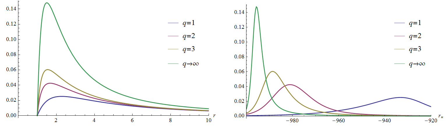
In Fig. 3 we plot the reduced eikonal part of the effective potential () as a function of the radial coordinate (left panel) and the tortoise coordinate (right panel).
As can be seen from examples presented in figure for special fixed values of and , the maximum of the effective potential is largest for case and smallest for case. The case with is in the middle. At large distances the effective potential tends to zero, as expected.
The second derivative with respect to the tortoise coordinate in the point of extremum is given by
| (5.22) | |||||
where , see (5.7). The calculation of second derivative gives us
| (5.23) |
where is defined in (5.19). We get
| (5.24) |
The last two terms in this relation may be simplified by using the relation for the third term in (5.19). We obtain
| (5.25) |
The square of the cyclic frequency in the eikonal approximation reads as following [10, 11]
| (5.28) |
where and . Here is the overtone number. By choosing an appropriate sign for we get the asymptotic relations (as ) on real and imaginary parts of complex in the eikonal approximation
| (5.29) | |||||
| (5.30) |
where (see (5.9)), , and is solution to master equation (5.20) and , where is defined in (5.27).
We note that the parameters of the unstable circular null geodesics around stationary spherically symmetric and asymptotically flat black holes are in correspondence with the eikonal part of quasinormal modes of these black holes. See [20, 21, 22] and references therein. Due to Ref. [23] this correspondence is valid if certain restrictions on perturbations are imposed.
6 Special cases and the limiting case
In this section we consider eikonal QNM for three cases when the master equation (5.20) may be solved in radicals for all values of and also in the limiting case .
6.1 The case
Let us consider the case (. In this case the master equation (5.20) is just a quadratic one with two roots:
| (6.1) |
Here
| (6.2) |
is belonging to interval , while is irrelevant for our consideration. We have
| (6.3) |
We get that the fuction is monotonically increasing and have the following limits: as and as . For all values we have
| (6.4) |
In this case the eikonal QNM (see (5.29) and (5.30)) read
| (6.5) | |||||
| (6.6) |
where , and is defined in (6.2).
| (6.7) | |||||
| (6.8) | |||||
where , and
| (6.9) |
Here corresponds to the position of the unstable, circular photon orbit in the Reissner-Nordström spacetime with the metric
| (6.10) |
where , with given by (6.9). Our AF (anisotropic fluid) metric (2.5) for is coinciding with the Reissner-Nordström one (6.10) when the following relation for radial coordinates is imposed.
6.2 The case
Now we put (). The master equation (5.20) in this case is just cubic one. It has a unique (real) solution for any belonging to interval
| (6.11) |
where
| (6.12) |
The function is monotonically decreasing from to and has the
asymptotics:
as
and as which imply
as and as .
It may be verified that the function
is monotonically inreasing from to .
6.3 The case
Let us consider the last case , when the master equation (5.20) of fourth power has a solution in radicals (which was obtained by Mathematica):
| (6.15) | |||
| (6.16) | |||
| (6.17) | |||
| (6.18) |
It may be verified that , given by relations (6.15)-(6.18), is real for all and obey . This property is graphically illustrated on Fig. 4.

6.4 The case
| (6.21) | |||||
| (6.22) |
where corresponds the position where the black hole effective potential attains its maximum. We note that is the radius of the photon sphere for the Schwarzschild black hole with the metric
| (6.23) |
which is coinciding with limiting case of our AF metric (2.5) when .
Remark. Here we restrict our choice of a test field by a massless (spin-zero, non-charged) scalar field which is the simplest “perturbation” to study. It may be shown that the consideration of a test Maxwell field on our black hole background will lead us to two equations on functions: and , which are certain combinations of coefficients (and their derivatives) coming from decomposing of vector potential in (vector) spherical harmonics. These equations (one of them is just an integrability condition) look like eq. (5.14) but with another potential , instead of (5.15)( in this case). Thus, we will obtain the same spectrum of QNM in eikonal approximation for a test Maxwell field as for a massless scalar field considered here.
7 Hod conjecture
Here we verify the conjecture by Hod [16] on the existence of quasi-normal modes obeying the inequality
| (7.1) |
where is Hawking temperature.
We note the Hod conjecture has been tested in theories with higher curvature corrections such as the Einstein-Dilaton-Gauss-Bonnet and Einstein-Weyl for the Dirac field (with positive result) [25]. (For negative result see Ref. [26].) Recently, we have also verified the Hod conjecture (with positive result) for a solution with dyon-like dilatonic black hole [27] for certain values of dimensionless parameter .
Here we verify this conjecture by using the obtained eikonal relations (5.30) for and the relation for the Hawking temperature (4.11). For our purpose it is sufficient to check the validity of the inequality
| (7.2) |
for all , , where is unique solution to master equation (5.20), which obeys , see Lemma in Appendix.
In (7.2) we use the limiting “eikonal value” given by the first term in (5.30) for the lowest overtone number .
Proposition 2. The dimensionless parameter from (7.2) obeys the inequality: for all and .
Proof. First we consider the case . In what follows we use the relation
| (7.3) |
for all and . Indeed, it follows from relations (A.16), (A.17) and (A.18) given at Appendix that
| (7.4) |
for all and . Thus, relation (7.3) is correct.
In what follows we use the following splitting
| (7.5) | |||||
| (7.6) |
where .
For we obtain from (7.3)
| (7.7) |
for all and . Now, we use the following fact about the function
| (7.8) |
where and . Namely, the function is monotonicall decreasing in . This follows from the relation
| (7.9) |
where and . This fact imlies for the following bound
| (7.10) |
for all and . Hence, we get
| (7.11) |
for all and .
The last bound
| (7.13) |
is also valid for all and . It follows from monotonical decreasing of the function in and . Here for and , are defined in Appendix.
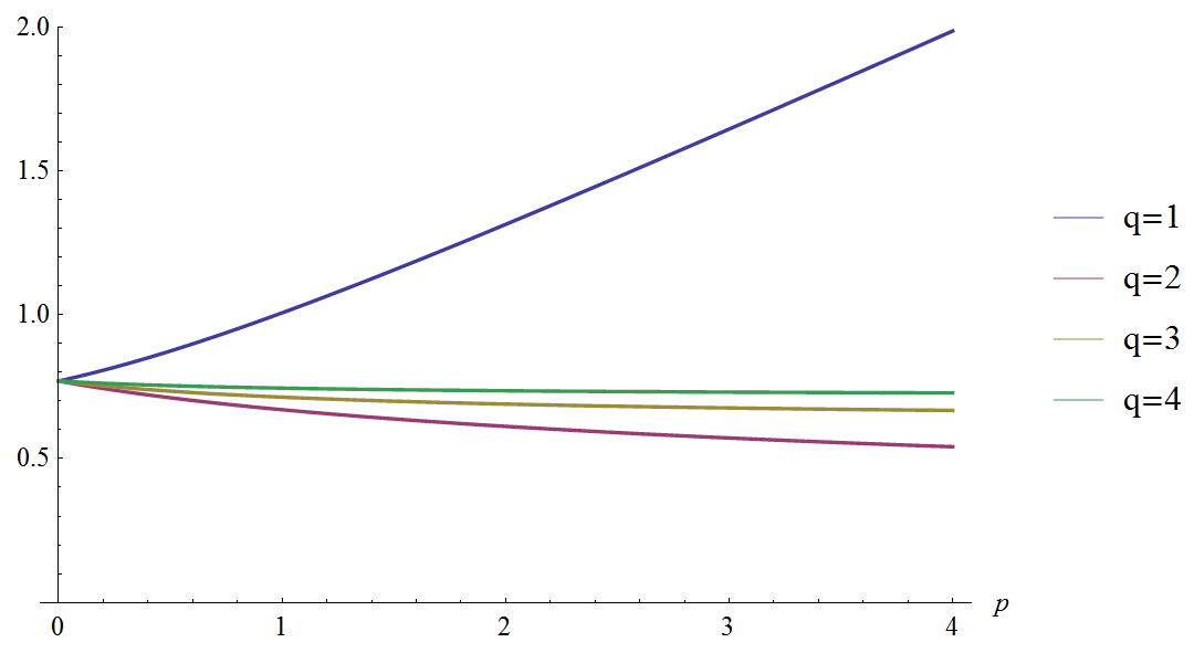
This result can be illustrated by a numerical plot of the function for a particular set of values of , depicted on Fig. 5. For the validity of Proposition 2 was verified numerically.
We note that recently, some examples of the violation of the Hod conjecture have been discussed for certain black hole solutions in supergravity and other theories [21].
Remark. Let us comment also on the case which gives us the Reissner-Nordström metric. It may be readily verified that in this case the inequality (7.2) is not satisfied for all values of : it is valid only for , where is some critical value of parameter [27]. As it was pointed out in [27] the violation of the Hod inequality in the eikonal regime for certain (and ) does not close the possibility for the obeying this relation for exact values of QNM for certain and all values of parameter .
8 Conclusion
Here we have studied a non-extremal black hole solutions in a 4-dimensional gravitational model with anisotropic fluid proposed in Ref. [1]. The equations of state for the fluid (1.4) contains a parameter which is natural number . We have outlined the global structure of solutions under consideration: for odd the Carter-Penrose diagram is coinciding with that of Reissner-Nordström metric (the case of time-like singularity hidden by two horizons) while for even it is coinciding with that of Schwarzschild metric (the case of space-like singularity hidden by one horizon). For the metric of the solution [1] coincides with the metric of the Reissner-Nordström solution while in the limit , we get the metric of the Schwarzschild solution. We have also presented certain physical parameters corresponding to BH solutions: gravitational mass , Hawking temperature, black hole area entropy.
We have examined the solutions to massless Klein-Fock-Gordon equation in the background of our static BH metric for given . . By using the tortoise coordinate we have reduced this equation to radial one governed by certain effective potential. This potential contains the parameters of solution such as , , natural parameter and also which is the multipole quantum number, .
Here we have studied the eikonal part of the effective potential for large and have found a master equation for the value , where is the value of the radial coordinate (radius) corresponding to the maximum of the eikonal part of the effective potential. By using the maximum value of (the eikonal part) of the effective potential and , we have calculated the cyclic frequencies of the QNMs in the eikonal approximation up to solution of the master equation in . Since the master equation is an algebraic equation of order in we were able to find analytical exact solutions for . For obtained values of eikonal QNMs we have also considered special cases and a limiting cases . For our (eikonal) relations are compatible with the well-known result for Reissner-Nordström solution [24] (for ), while for they in an agreement with the well-known result for the Schwarzschild solution [5].
We have also tested the validity of the Hod conjecture for our solutions by considering QNMs (eikonal) frequences with the lowest value of the overtone number . We have shown that the Hod conjecture is valid in the range of . This assumption is valid for these values of since it is supported by examples of states with large enough values of the multipole number .
We note, that the results obtained here for eikonal QMN modes of test massless (non-charged) scalar field are also valid for some other test fields, e.g. for electromagnetic one. This may be considered (by product) in a separate publication. (The results of Refs. [28, 29] may be also used in future work.)
A Appendix
Here we prove the Proposition 1. Since the extremality condition (5.18) for the effective potential () is equivalent to the master equation (5.20) (), and the second derivative at the point of extremum is given by relation (5.26) with (see (5.21)), the Proposition 1 is equivalent to the following Lemma.
Lemma. For any and , the master equation
| (A.1) |
has only one solution , belonging to interval . This solution obeys the inequality
| (A.2) |
for all and .
Proof. Since is not a solution to eq. (A.1) we present the master equation in the following form
| (A.3) |
. The functions , , are presented at Fig. 6. It follows from the definition (A.3) that
| (A.4) |
for , and
| (A.5) |
| (A.6) |
for all . Hence the seminterval should be excluded in our search the solution to Eq. (A.3).
Let us analyze behavior of the function for and fixed . The first derivative reads
| (A.7) |
For , we have for and hence the function is monotonically increasing from to , when . By applying the Intermediate Value Theorem to our continuous monotonically increasing function , , we get that for any there exist unique , with , which obeys eq. (A.1). 11footnotetext: We remind that the Intermediate Value Theorem states that if is a continuous function defined on the interval , then it takes on any given value between and at some point of this interval. Inequality (A.2) is obviously satisfied for . That means that the Lemma is valid for .
Now we consider the case . From (A.7) we obtain that the there exists a unique point of extremum of the function in the interval
| (A.8) |
, which is the first root of the quadratic equation . The second root is irrelevant for our consideration.
The calculations give us: , , and , , . We note that
| (A.9) |
for all . This follows from monotonical decreasing of the function for , since and
| (A.10) |
is monotically increasing in for .

The function (for ) is monotonically increasing in the interval , since in this interval, see (A.7), while it is monotonically decreasing in the interval due to inequality which is valid there. Hence we get
| (A.14) |
for all and . This implies that the semi-interval should be excluded in our search of solution to equation (A.3) for a given . Thus, we restrict our consideration to .
Let us define , which obeys the following equation
| (A.15) |
. By applying the Intermediate Value Theorem for a continuos monotonically increasing function defined on and using (A.5) and (A.14) one can readily prove that such point does exist and is unique for any .
The calculations give us
| (A.16) |
It may be proved that
| (A.17) |
for any natural . Indeed, if we suppose that for some we get from monotonical increasing of the function in and obvious inequality for that
and hence we come to a contradiction. Thus, the chain of inequalities (A.17) is correct.
Now we return to our original equation (A.3). From monotonical increasing of the function in we get that for and hence the semi-interval should be excluded for our consideration of (A.3). By applying once more the Intermediate Value Theorem for a continuos monotonically increasing function defined on and using (A.5) and (A.15) we can find that the point which obeys the equation (A.3) does exist, belongs to and is unique for any and . We denote this point as . Thus, we have
| (A.18) |
for all and . It follows from (A.11) and (A.18)
| (A.19) |
as uniformly in .
We note that one can present the solution as
| (A.20) |
where is the function which is inverse to the function , defined as . The function is a continuos and monotonically increasing one (due to a proper theorem on inverse function). It may be readily verified that
| (A.21) |
and
| (A.22) |
Thus, the first part of the Lemma is proved for all . Now, we should prove the second part of the Lemma for (for it was checked above). Let us consider the function
| (A.23) |
for and . We get
| (A.24) |
where and are defined by relations (A.8) and (A.10), respectively. We find that for all and hence for with and . We remind that for all and . Thus, the inequality (A.2) is satisfied. The Lemma is proved.
Acknowledgments
This paper has been supported by the RUDN University Strategic Academic Leadership Program (recipients: V.D.I. - mathematical model development and S.V.B. - simulation model development). The reported study was partially funded by RFBR, project number 19-02-00346 (recipients S.V.B. and V.D.I. - physical model development).
References
- [1] H. Dehnen, V. D. Ivashchuk and V. N. Melnikov, On black hole solutions in model with anisotropic fluid, Grav. Cosmol. 9, 153 (2003); arXiv:gr-qc/0211049.
- [2] C.V. Vishveshwara, Nature 227(5261), 936 (1970). DOI 10.1038/227936a0
- [3] W.H. Press, Astrophys. J. Lett. 170, L105 (1971). DOI 10.1086/180849
- [4] S. Chandrasekhar, S. Detweiler, Proceedings of the Royal Society of London Series A 344(1639), 441 (1975). DOI 10.1098/rspa.1975.0112
- [5] H.J. Blome, B. Mashhoon, Physics Letters A 100(5), 231 (1984). DOI 10.1016/0375-9601(84)90769-2
- [6] V. Ferrari, B. Mashhoon, Phys. Rev. Lett.52(16), 1361 (1984). DOI 10.1103/PhysRevLett.52.1361
- [7] V. Ferrari, B. Mashhoon, Phys. Rev. D30(2), 295 (1984). DOI 10.1103/PhysRevD.30.295
- [8] K.D. Kokkotas, B.G. Schmidt, Living Reviews in Relativity 2(1), 2 (1999). DOI 10.12942/lrr-1999-2
- [9] H.P. Nollert, Classical and Quantum Gravity 16(12), R159 (1999). DOI 10.1088/0264-9381/16/12/201
- [10] E. Berti, V. Cardoso, A.O. Starinets, Classical and Quantum Gravity 26(16), 163001 (2009). DOI 10.1088/0264-9381/26/16/163001
- [11] R.A. Konoplya, A. Zhidenko, Reviews of Modern Physics 83(3), 793 (2011). DOI 10.1103/RevModPhys.83.793
- [12] Y. Hatsuda, Phys. Rev. D101(2), 024008 (2020). DOI 10.1103/PhysRevD.101.024008
- [13] B.P. Abbott et al, Phys. Rev. Lett. 116(6), 061102 (2016). DOI 10.1103/PhysRevLett.116.061102
- [14] B.P. Abbott et al, Physical Review X 9(3), 031040 (2019). DOI 10.1103/PhysRevX.9.031040
- [15] B.P. Abbott et al, Astrophys. J. Lett. 892(1), L3 (2020). DOI 10.3847/2041-8213/ab75f5
- [16] S. Hod, Phys. Rev. D75(6), 064013 (2007). DOI 10.1103/PhysRevD.75.064013
- [17] K. A. Bronnikov and S. G. Rubin, Black Holes, Cosmology, and Extra Dimensions (World Scientic, Singapore, 2008).
- [18] S. V. Bolokhov, V. D. Ivashchuk. In: Proc. of the Twelfth Asia-Pacific International Conference on Gravitation, Astrophysics, and Cosmology. pp. 327-331 (World Scientific, Singapore, 2016).
- [19] J.W. York, Phys. Rev. D 31, 775 (1985).
- [20] V. Cardoso, A.S. Miranda, E. Berti, H. Witek, V.T. Zanchin, Phys. Rev. D79(6), 064016 (2009). DOI 10.1103/PhysRevD.79.064016
- [21] M. Cvetič, G.W. Gibbons, C.N. Pope, Phys. Rev. D94(10), 106005 (2016). DOI 10.1103/PhysRevD.94.106005
- [22] K.S. Virbhadra, G.F.R. Ellis, Phys. Rev. D62(8), 084003 (2000). DOI 10.1103/PhysRevD.62.084003
- [23] R.A. Konoplya, Z. Stuchlik, Physics Letters B 771, 597 (2017). DOI 10.1016/j.physletb.2017.06.015
- [24] N. Andersson, H. Onozawa, Phys. Rev. D54(12), 7470 (1996). DOI 10.1103/PhysRevD.54.7470
- [25] A.F. Zinhailo, European Physical Journal C 79(11), 912 (2019). DOI 10.1140/epjc/s10052-019-7425-9
- [26] M.A. Cuyubamba, R.A. Konoplya, A. Zhidenko, Phys. Rev. D93(10), 104053 (2016). DOI 10.1103/PhysRevD.93.104053
- [27] A.N. Malybayev, K.A. Boshkayev, V.D. Ivashchuk, The European Physical Journal C, 81: 475 (12 pages) (2021). DOI: 10.1140/epjc/s10052-021-09252-z
- [28] M.S. Churilova, European Physical Journal C 79(7), 629 (2019). DOI 10.1140/epjc/s10052-019-7146-0
- [29] R.A. Konoplya, A. Zhidenko, A.F. Zinhailo, Classical and Quantum Gravity 36(15), 155002 (2019). DOI 10. 1088/1361-6382/ab2e25