Influence of the heliospheric current sheet on the evolution of solar wind turbulenceJournal: ApJMatplotlib (Hunter 2007)
Abstract
The effects of the heliospheric current sheet (HCS) on the evolution of Alfvénic turbulence in the solar wind are studied using MHD simulations incorporating the expanding-box-model (EBM). The simulations show that near the HCS, the Alfvénicity of the turbulence decreases as manifested by lower normalized cross helicity and larger excess of magnetic energy. The numerical results are supported by a superposed-epoch analysis using OMNI data, which shows that the normalized cross helicity decreases inside the plasma sheet surrounding HCS, and the excess of magnetic energy is significantly enhanced at the center of HCS. Our simulation results indicate that the decrease of Alfvénicity around the HCS is due to the weakening of radial magnetic field and the effects of the transverse gradient in the background magnetic field. The magnetic energy excess in the turbulence may be a result of the loss of Alfvénic correlation between velocity and magnetic field and the faster decay of transverse kinetic energy with respect to magnetic energy in a spherically expanding solar wind.
Keywords:
Interplanetary turbulence (830), Solar wind (1534), Magnetohydrodynamical simulations (1966)I Introduction
Turbulence is a pervasive phenomenon in fluids and plasmas and has been observed to be a major feature of the solar wind. It is thought to be one of the main processes leading to solar wind heating (Kiyani et al. 2015, e.g.) and contribute to its acceleration from the solar corona (Belcher 1971; Leer et al. 1982, e.g.), while also affecting the acceleration and transport of energetic particles. Thus, understanding the origin and evolution of solar wind turbulence is crucial for fully understanding the heliosphere as a whole.
Coleman 1968, using Mariner 2 data, showed that the power spectra of fluctuations in the solar wind have power-law scaling relations, indicating a well-developed turbulence. Belcher & Davis 1971 found that these fluctuations are mainly outward-propagating Alfvén waves, with nearly-incompressible plasma density and magnetic field. An important question is how the Alfvénic fluctuation, or Alfvénic turbulence, evolves radially. Wentzel-Kramers-Brillouin (WKB) (Alazraki & Couturier 1971; Belcher 1971; Hollweg 1974, e.g.) theory of the radial evolution of the Alfvén wave amplitude was developed. Non-WKB (Heinemann & Olbert 1980; Barkhudarov 1991; Velli 1993, e.g.) theory shows that linear coupling between the outward- and inward-propagating Alfvén waves leads to frequency-dependent reflection of the waves. Magnetohydrodynamic (MHD) models were developed on the evolution of the turbulence spectra and other parameters such as the wave energy densities (Tu et al. 1984; Zhou & Matthaeus 1990; Zank et al. 1996, e.g.).
Elsässer varibles , where and are velocity and magnetic field expressed in Alfvén speed, i.e. with and being the magnetic field and plasma density, are convenient in describing the Alfvénic fluctuations as they represent the inward and outward propagating Alfvén waves respectively. Two quantities have been used as important diagnostics of the Alfvénic turbulence, namely the normalized cross helicity () defined as:
| (1) |
and normalized residual energy () defined as:
| (2) |
measures the relative amount of outward and inward wave energies and measures the relative amount of kinetic and magnetic energies. A large number of works were conducted on the radial evolution of these two quantities in the solar wind (Roberts et al. 1987; Bavassano et al. 1998; Bruno et al. 2007; Chen et al. 2020; Shi et al. 2021, e.g.) but two outstanding problems remain unresolved. First, the normalized cross helicity decreases with radial distance to the Sun, and second, a prevailing negative value of residual energy is observed. It is known that, in a homogeneous medium with a uniform background magnetic field, the Alfvénic turbulence evolves toward a status that only one wave population survives, i.e. . This is the so called “dynamic alignment” (Dobrowolny et al. 1980). In contrast to the theory, in the solar wind, the dominance of the outward Alfvén wave is gradually weakened during the radial propagation as manifested by the decrease of . Besides, in a purely Alfvénic system, the kinetic and magnetic energies should be exactly equi-partitioned, i.e. , while in the solar wind, a magnetic energy excess is typically observed even at distances very close to the Sun, below 30 solar radii (Chen et al. 2020; McManus et al. 2020; Shi et al. 2021).

One possible mechanism that resolves these paradoxes is the large-scale velocity shear in the solar wind. Coleman 1968 proposed that the differential streaming generates Alfvén waves at long wavelengths. These newly-generated waves do not have a preferential propagating direction and thus the initial dominance of the outward wave gradually declines. This shear-driven decrease of cross helicity was confirmed by numerical simulations (Roberts et al. 1992; Shi et al. 2020). Velocity shear is widely adopted in turbulence models as a source for the wave energies and is able to reproduce the observed decrease of in the models. On the contrary, there has been no satisfactory solar wind turbulence model that leads to negative residual energy so far. For example, in the model by (Zank et al. 2017), the source term for the residual energy is attributed to the stream shear but whether this term causes growth or decay of the residual energy is arbitrary. Heliospheric current sheet (HCS) is a good candidate that may influence the evolution of Alfvénic turbulence. It is shown by both simulations and in-situ observations that in the proximity of the HCS, the Alfvénicity of the turbulence decreases in general (Goldstein & Roberts 1999; Chen et al. 2021, e.g.). However, how the HCS modifies the dynamic evolution of and in the spherically expanding solar wind is still unclear.
In this study, we carry out two-dimensional MHD simulations using the expanding-box-model (EBM). Large-scale solar wind structures, including the fast-slow stream interaction regions (SIRs) and the HCS, are constructed and evolve self-consistently in the simulations. We investigate how properties of the Alfvénic turbulence evolve radially and how SIRs and HCS modify its evolution. A superposed-epoch analysis of HCS crossings at 1 AU is carried out using the OMNI dataset and the turbulence properties near the HCS are examined. The paper is organized as follows. In Section II we present the setup of the MHD simulations and the numerical results. In Section III we present the superposed-epoch analysis of the HCS crossings observed at 1 AU. We then discuss our results in Section IV and conclude in Section V.

II Expanding-Box-Model simulation
II.1 Numerical method and 1D test run
The code we use for simulations is a 2D pseudo-spectral MHD code used by Shi et al. 2020 to study the interaction between SIRs and turbulence. EBM module is implemented so that the radial expansion effect of the solar wind is taken into account (Grappin et al. 1993; Grappin & Velli 1996). The expansion effect is not negligible in the solar wind because it induces inhomogeneity of the background streams, which leads to the reflection of the Alfvén waves (Heinemann & Olbert 1980, e.g.), and anisotropic evolution of velocity and magnetic fields in the radial and transverse directions (Dong et al. 2014, e.g.). The EBM has also been employed to reproduce the “magnetic switchbacks” observed in the young solar wind (Squire et al. 2020). In our code, a finite spiral angle of magnetic field and stream interface is allowed so that compression and rarefaction regions are constructed. A detailed description of the numerical method can be found in Shi et al. 2020.
We carried out four simulations with two free parameters, namely whether a non-zero spiral angle is set and whether the expansion effect is included. Here we mainly present results from the run with both a non-zero spiral angle and the expansion effect, i.e. the most realistic run. The parameters for the initial setup are chosen according to solar wind observations as described below. The simulation starts from and ends at where is the solar radius. The initial spiral angle is so that the angle becomes at 1 AU. The size of the simulation domain is where is the corotating coordinate system, i.e. is parallel to the background magnetic field and is the quasi-longitudinal direction (Shi et al. 2020). means that the domain is a full circle in the ecliptic plane. The initial background fields as functions of the quasi-longitudinal direction are plotted in the left column of Figure 1 with normalized units. The quantities for normalization are: cm-3, nT, , km/s, and nT. The wind consists of two fast streams and two slow streams. The transition between fast and slow streams is of the form where . The velocity of the streams is purely radial with the speed ranging from 340 km/s to 700 km/s. We note that in Figure 1 the velocity is in the reference frame of the expanding box, which moves radially with the average speed of the plasma inside the simulation domain km/s. The density is 360 for the slow streams and 140 for the fast streams. Two Harris current sheets with thickness are embedded in the center of the slow streams. The current sheets are force-free, as the in-situ measurement of the HCS usually shows (Smith 2001), and a finite -component is used to make sure that is constant and the magnetic field strength is uniformly nT. The pressure is uniform and equals 5 nPa, i.e. the plasma beta is , so that the temperatures of the fast and slow streams are MK and MK respectively. The adiabatic index is set to be instead of since the solar wind observations show that the cooling rate of the solar wind is slower than a adiabatic cooling (Hellinger et al. 2011, e.g.).

In Figure 1, we show the evolution of the background fields from a 1D run with grid points on -axis, i.e. the quasi-longitude direction. Top row shows density (blue) and temperature (orange), middle row shows the radial component (blue) and transverse component (orange) of the velocity, bottom panel shows the radial component (blue), out-of-plane component (orange), and the magnitude (black) of the magnetic field. From left to right columns are the profiles of the background fields at three locations as labeled on the top. In each column, the green shade shows one of the two compression regions and the vertical dashed line marks one of the polarity reversal points of the radial magnetic field. We can see that, as the simulation proceeds, a compression region with enhanced density, temperature, and magnetic field strength forms between the trailing fast stream and leading slow stream. A divergent transverse flow due to the deflection of the streams is also observed in the compression region. In the rarefaction region, i.e. the trailing edge of the fast slow, the density, temperature, and magnetic field strength decrease. But we note that near the current sheet, a dip is seen in density and temperature but the magnetic field strength shows a peak. This is a result of the differential decay rates of and induced by the expansion of the solar wind. As decays slower than , an initial force-free current sheet cannot maintain a uniform magnetic pressure once the expansion starts and a local peak of magnetic pressure forms at the polarity reversal point. The large magnetic pressure will then push the plasma away from the current sheet, resulting in a local dip in density and temperature and also a divergent transverse flow.

II.2 Results of the 2D runs with waves
Based on the 1D run, 2D simulations are conducted. At initialization, circularly-polarized Alfvénic wave bands comprising 16 modes are added on top of the background streams with wave vectors parallel to and correlated & fluctuations in & directions (see (Shi et al. 2020) for more details). The energy spectrum of the initial waves obeys with where , i.e. the longest and shortest wavelengths are (wave period hr) and (wave period min) respectively. Both outward and inward waves are added with the amplitude of inward waves being of the amplitude of outward waves. The amplitude of the first mode of outward waves is nT. To avoid sharp jumps of perturbation fields across the current sheets, we modulate the wave amplitudes by a hyperbolic tangent function, similar to the -component of the background magnetic field, such that the wave amplitudes are exactly 0 at the center of the current sheets. Note that this requires non-zero wave components along inside the current sheets to ensure . The number of grid points is (we note that the simulation domain size is ) so that the smallest wavelength that is resolved is , corresponding to a wave period s, which is approximately two magnitudes larger than the ion gyro-scale and ion inertial scale. But we note that in the MHD simulations, there are no intrinsic gyro-scales and inertial scales, or in other words these kinetic scale lengths are zero in MHD.
We process the simulation data using the same method as described in (Shi et al. 2020). At each time, or radial distance to the Sun equivalently, we first calculate the -averaged fields, i.e. the background fields. Then we remove the background fields to get the wave fields. We only analyze wave components that are perpendicular to the plane background magnetic field . We note here that in the plane, the background magnetic field is always aligned with as the axis rotates away from the radial direction as the solar wind expands (Shi et al. 2020). The perturbed Elsässer variables are defined by
| (3) |
We then apply Fourier transform along to , , and . As there are 2048 grid points along , 1024 wave modes are resolved with wave-numbers , i.e. mode corresponds to . We divide all the wave modes into 10 wave-number bands which are logarithmically spaced, i.e. band contains modes , or wavelengths between and . We then calculate and for each wave-number band and also for integration of all wave modes.
In Figure 2 we present the profiles color-coded with (top row) and (bottom row) for all wave modes (left column) and for band 03 (right column) which corresponds to wave length , or roughly wave period min. The figure is produced by piling up the profiles of at different moments or equivalently different radial locations . In top-left panel, we mark the boundaries of fast streams, defined as at which the background radial speed equals 650 km/s, by dashed white lines and mark the boundaries of slow streams, defined as at which the background radial speed equals 400 km/s by dashed black lines. The two current sheets are located in the center of the slow streams, around and . We first inspect the left column of Figure 2 which shows and calculated using wave energies integrated over all wave-numbers. As already discussed by Shi et al. 2020, in regions with nearly uniform background fields, i.e. inside fast streams and inside slow streams far from the current sheets, remains almost constant throughout the evolution, indicating that the Alfvénicity remains high in these regions. In the velocity-shear regions (regions between the black and white lines), declines with radial distance. Especially, in the compression region (around and ), drops below 0 beyond . Shi et al. 2020 showed that in shear regions, the damping of the outward Alfvén wave is significantly faster than the inward Alfvén wave, leading to the decrease in . Except for near the current sheets, which will be discussed in detail later, oscillates around 0 in all regions, indicating that the Alfvénicity of the waves is well conserved for the long wavelength modes (we note that the integrated wave energies are dominated by the modes of largest scales). The oscillation in is caused by periodic correlation and de-correlation between the outward and inward waves. From the left column of Figure 2, we also see that the evolution of Alfvén waves is significantly modified by the current sheets. In the neighborhood of the current sheets, decreases quite fast and evolves toward negative values. In the left panel of Figure 3 we plot the radial evolution of and in a band of width around the current sheet initially located at . starts from a high value, i.e. 0.92 determined by the initial condition, drops to around 0.2 within 100 and then remains stable. starts from exactly 0, rises slightly at the beginning due to the increase of kinetic energy caused by the magnetic pressure gradient at the current sheet as discussed in Section II.1, and then starts to drop continuously, reaching a value at 1 AU. For comparison, we plot the time evolution of and from the run without expansion in the right panel of Figure 3. Evolution of does not show much difference between the two runs while remains around 0 in the run without expansion, indicating that expansion effect is important to the decrease of around the current sheet, which will be discussed in more detail in Section IV.
In the right column of Figure 2, we show the profiles of and for wave band 03. Compared with the left column, the drop of in velocity-shear regions is much more significant and the -drop regions around the current sheets are wider. For , the most prominent feature is that inside the compression regions, evolves toward , i.e. kinetic energy becomes dominant in these regions, indicating that the large-scale velocity shear and compression facilitate the transfer of kinetic energy toward small scales.
In Figure 4 we show the -spectra, i.e. the parallel spectra, of various fields calculated at the moment . From left to right columns are spectra averaged in -bands of width inside fast stream, current sheet and compression region respectively. Top row shows the spectra of outward (blue) and inward (orange) Elsässer variables. Middle row shows the spectra of kinetic (blue) and magnetic (orange) perturbations. We multiply these spectra by as the “critical balance” model (Goldreich & Sridhar 1995) predicts a parallel spectrum . We can see from Figure 4 that in general these spectra are steeper than the prediction of the critical balance model except for inside the fast stream. This is because the shears in magnetic field and velocity turn the wave vector from quasi-parallel to quasi-perpendicular and enlarges the perpendicular wavenumber gradually which speeds up the dissipation of the wave energies (Shi et al. 2020). Bottom row shows the spectra of and calculated from the spectra shown in top and middle rows. Inside the fast stream, is close to 1 and is close to 0 for most modes, except for close to the numerical dissipation range, meaning that the waves maintain a high Alfvénicity over a large span of wave numbers. Around the current sheet, decreases to nearly 0 for all wave numbers. is negative for most of the wave numbers, except for an intermediate range () where it is around 0. In the compression region, is overall smaller than the initial condition 0.92 but the curve of shows a decrease with at small wave numbers and rises again. is around 0 for small wave numbers and shows a significant increase with , reaching its maximum value at the same where reaches its local minimum. It indicates that in the compression region the large scale stream structure generates small-scale fluctuations that are kinetic energy dominated, as observed in previous simulations (Roberts et al. 1992, e.g.). The newly-generated fluctuations weaken the dominance of the outward Alfvén waves, consistent with the scenario proposed by Coleman 1968. We note that for large wave-numbers () the spectra are significantly modulated by the explicit numerical filter applied to the simulation, thus spectral breaks can be seen at large wave-numbers.
We do not present the perpendicular power spectra for the following reasons. First, as the simulation coordinate system is non-Cartesian, there is no axis perpendicular to . The axis is perpendicular to initially but the angle between and gradually increases (Shi et al. 2020). Second, because of the elongated simulation domain along and also due to the spherical expansion, the resolution in is much lower than that in . Besides, as we would like to focus on certain longitudinal regions, e.g. around the HCS, instead of the whole range, the number of data points is limited. Because of the above reasons, it is difficult to produce physically meaningful perpendicular spectra.

In Figure 5, we plot the -profiles of the normalized density fluctuation (blue) and the square of Mach number (orange) in the simulation at moment . Here and are the root-mean-squares of density and velocity calculated long . is the sound speed. Yellow and green shades mark the fast and slow streams respectively. The vertical dashed lines are the locations of the current sheets. The normalized density fluctuation is overall small, mostly below 0.2, similar to the solar wind observation (Shi et al. 2021, e.g.). In the compression region and near the current sheet, e.g. from , is highly correlated with , implying a large compressive component in the velocity fluctuations in these regions.
III Superposed-epoch analysis of HCS at 1 AU
Although works have been carried out on turbulence properties around SIRs (Borovsky & Denton 2010, e.g.), literature on how HCS affects the solar wind turbulence is still incomplete. To validate our simulation results, we carry out a superposed-epoch analysis of HCS crossings at 1 AU and study how the properties of turbulence change near HCS.
III.1 Selection and structure of HCS
For the current study, we use the OMNI dataset, which contains magnetic field and plasma data from multiple spacecraft, including ACE and WIND (King & Papitashvili 2005). Time resolution of the data is 1 minute, enough for study of MHD turbulence. We analyze data during two 4-year periods: 2000-2003 which is around solar maximum of solar cycle 23, and 2007-2010 which is around solar minimum between solar cycles 23 & 24, as shown by the shaded regions in Figure 6, which plots monthly sunspot number.
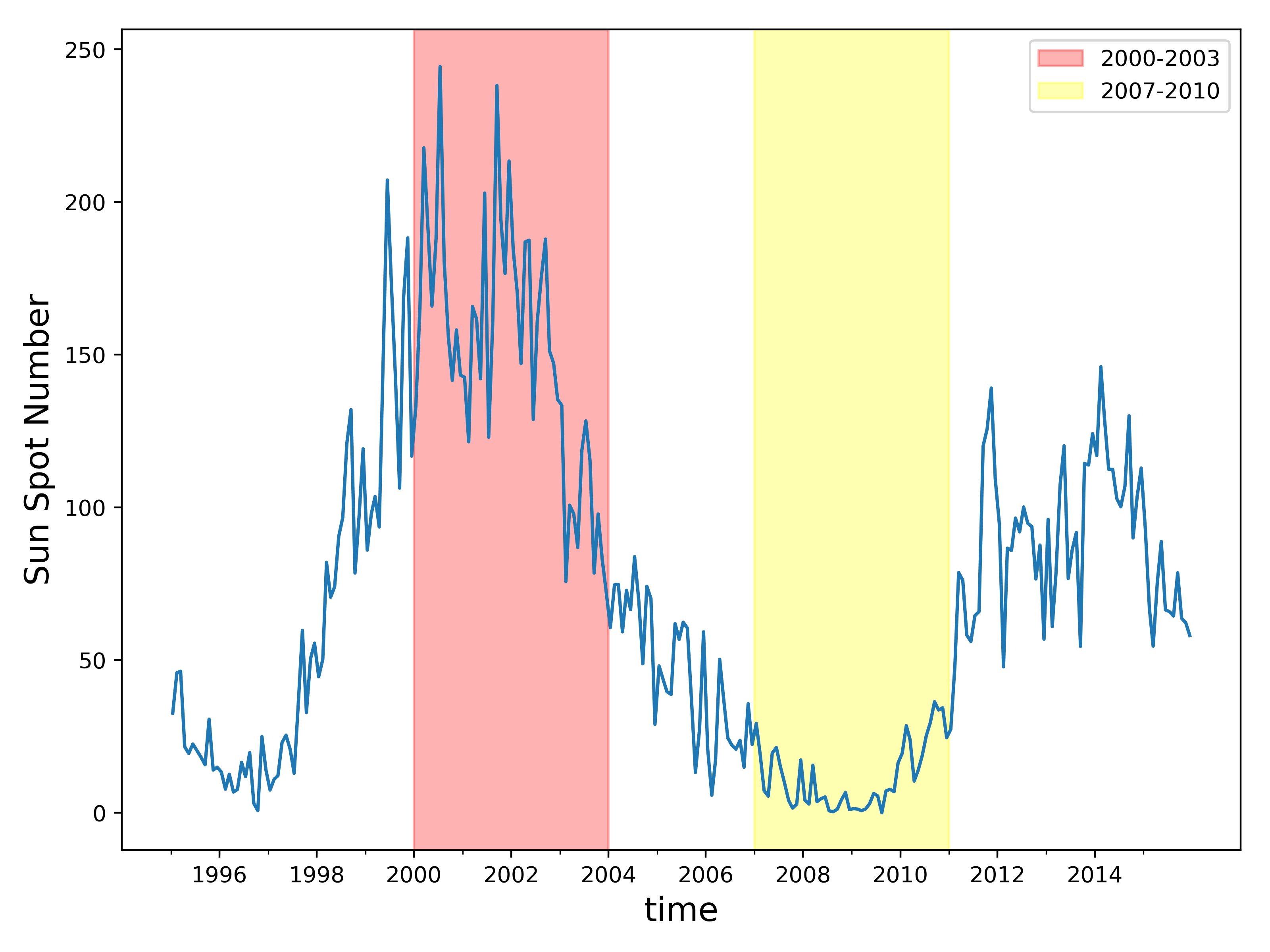

The procedure to select HCS crossings is stated as follows. We first calculate the one-day average of , which is equivalently the opposite of radial component of the solar wind magnetic field. Then we find days when its polarity changes and we require that the polarities before and after each polarity-reversal day maintain at least 4 days. Then we inspect the 1-minute data to determine the exact polarity reversal times. We identify 48 events for solar maximum and 45 events for solar minimum. List of the HCS crossings is shown in Table 1.
Superposed-epoch analysis of the HCS structure is shown in Figure 7. From top to bottom rows are GSE , GSE , , GSE , proton density, and proton temperature respectively. Left column is solar maximum and right column is solar minimum. In each panel, grey curves are individual events and blue curve is the median value of all events. In the top two rows we also plot medians of the magnetic field strength in black curves. We have reversed the time series of certain events such that is always changing from negative to positive. The time scale for HCS crossings is on average 1-2 hours and the HCS is embedded in much thicker (1-2 days) plasma sheets with enhanced proton density and lower proton temperature. The magnetic field strength is quite constant across the HCS, implying a force-free structure. By comparing left and right columns of Figure 7, we see that the strength of magnetic field is larger in solar maximum than solar minimum. Another thing to notice is that there is a negative GSE at the HCS, i.e. the plasma flow is rotating in the same direction with the solar rotation. The reason might be that HCS is usually embedded in slow solar wind ahead of the compression region and are pushed along longitudinal direction in accordance with solar rotation (Eselevich & Filippov 1988; Siscoe 1972).
III.2 Turbulence properties near HCS

We then analyze turbulence properties near the HCS. We use a running time window of width 128-min. A time window with data gap ratio larger than 20% is not considered. Inside each time window, we first apply linear interpolation to velocity, magnetic field, and proton density to fill the data gaps. Then we calculate Elsässer variables after determining the polarity of radial magnetic field by averaging in the time window. Finally, we apply Fourier transform to these fields. Similar to the process of simulation data in the prior section, we divide the frequency into 6 bands such that band contains wave modes , e.g. wave band 6 contains waves whose periods are between 128/=4 min and =2 min. We calculate and for each wave band by integrating wave energies in each band. In addition, we fit the power spectra and get the spectral slopes for velocity, magnetic field, outward and inward Elsässer variables.
In Figure 8, we show superposed-epoch analysis of (top row) and (bottom row). Left column is solar maximum and right column is solar minimum. Colors represent different wave bands such that dark to light colors are bands 1-6. We see that in general decreases with frequency while increases with frequency. Top-left panel shows that in a time window 1 day, approximately the width of the plasma sheet, drops as we approach the center of HCS. In a narrow window of width comparable to the thickness of HCS, i.e. 1-2 hours, drops significantly since the outward and inward waves mix with each other. Bottom-left panel of Figure 8 shows slightly decrease of inside the plasma sheet while a large drop of is observed near HCS. In solar minimum (right column of Figure 8), the above results qualitatively hold but both and are lower compared with solar maximum.
In Figure 9, we show the superposed-epoch analysis of various spectral slopes. Again, left and right columns are solar maximum and solar minimum respectively. In the top row, blue and orange curves are spectral slopes of velocity and magnetic field. In the bottom row, blue and orange curves are spectral slopes of outward and inward Elsässer variables. In each panel, the two horizontal dashed lines mark the values and for reference. Away from the HCS, velocity spectrum has a slope near and magnetic field spectrum has a slope near as typically observed in the solar wind (Chen et al. 2020; Shi et al. 2021, e.g.). Near the center of HCS, both of the two spectra steepen and the steepening is more pronounced in solar maximum. The outward Elsässer variable has a spectral slope near and shows a slight steepening near HCS in solar maximum while no obvious steepening is observed in solar minimum. The variation in spectral slope of inward Elsässer variable is more dramatic compared with the other quantities. spectrum is quite flat far from the HCS, around in solar maximum and in solar minimum. We note that, in our simulation (top-left panel of Figure 4), a flatter spectrum compared with the spectrum is also observed. At the center of HCS, the inward and outward Elsässer variables have the same slope as expected since the two wave populations are not well separated near the polarity-reversal time.

In Figure 10, we plot the superposed-epoch analysis of the normalized density fluctuation (blue) and the square of the velocity fluctuation Mach number (orange). In solar minimum, the two quantities are highly correlated while in solar maximum they are correlated only close to the HCS. We note that our simulation result (Figure 5) also shows high correlation between the two parameters close to the current sheets. However, in the simulation, the density fluctuation is smaller near the HCS compared with the surroundings, in contrast to the observation. The reason is that in the initial condition of the simulation we artificially decrease the perturbation amplitude close to the HCS to avoid discontinuity in the perturbation fields. The increase of the density fluctuation near the HCS from OMNI data might be related to the tearing instability of HCS close to the Sun which ejects bunches of flux ropes from the tip of helmet streamers (Réville et al. 2020).

IV Discussion
We compare the simulation results from Section II and the superposed-epoch analysis from Section III. In the simulation, drops in a wide longitudinal range around the current sheet (Figure 2), which is also observed at 1 AU (Figure 8). Similarly, in both simulation and observation, drops in the neighbourhood of HCS. Grappin et al. 1991 analyzed four-month of Helios 1 data and found that within the neutral sheet, the turbulence properties are close to the “standard”, or fully-developed, MHD turbulence, rather than Alfvénic turbulence. Standard MHD turbulence is characterized by balanced outward/inward Elsässer energies and an excess of magnetic energy, consistent with our results. In this scenario, the background magnetic field dissipates the residual energy (the so-called “Alfvén effect”) which is a correlation between the two Elsässer variables generated by intrinsic nonlinear interaction. In other words, the Alfvén effect is essentially the dissipation of two colliding (correlated) counter-propagating Alfvén wave packets as first described by Kraichnan 1965, and hence it is determined by the background magnetic field strength along the wave propagation direction. Thus, the absolute value of the residual energy, regardless of its sign, is larger inside current sheets where the Alfvén effect is weaker. Grappin et al. 1991 explained the balance between outward/inward Elsässer energies at small scales by the fact that the injected energy at large scales due to velocity shear is balanced in and . This interpretation, however, cannot explain the decrease in around the current sheet in our simulation because there is no such energy source near the current sheet in the simulation. Instead, the decrease of around the HCS in the simulation is likely to be a result of the shear of background magnetic field which deforms the wave fronts and facilitates the dissipation of wave energies, similar to the velocity shear effect. In addition, Grappin et al. 1991 does not answer the question why the residual energy is negative instead of positive in the current sheets. Here we propose a mechanism related to the expansion effect of the solar wind. Near the HCS, the weak background magnetic field allows fluctuations to evolve freely so they are dominated by the spherical expansion effect, which leads to , and consequently . Hence, as the radial distance increases, the transverse magnetic field fluctuation (in Alfvén speed) becomes larger than the transverse velocity fluctuation, leading to a negative . This mechanism is supported by Figure 3 which shows that without expansion no net residual energy is produced. Meanwhile, Figure 3 also shows that the decrease of cannot be explained by expansion effect and must be caused by processes related to the shear of the background magnetic field.
We note that, our simulation cannot explain why in the solar wind is generally negative even far from HCS as can be seen from Figure 8. Recent studies using Parker Solar Probe data show that is already negative at below 30 solar radii while is increasingly high as the satellite moves closer to the Sun (Chen et al. 2020; Shi et al. 2021). Our results show that the presence of a current sheet indeed leads to a dominance of magnetic energy, but it also results in a decrease in . Thus the observed population of the solar wind fluctuations (D’Amicis & Bruno 2015, e.g.) is possibly Alfvénic turbulence evolved under the influence of current sheets, while the prevailing population may be generated in the very young solar wind with other processes taking effect or it may be a natural result of the evolutin of Alfvénic turbulence (Boldyrev et al. 2011, e.g.).
Last, we would like to comment that, the statistical study of Alfvénic turbulence properties near SIRs by Borovsky & Denton 2010 shows results quite different from our simulations. Their Figure 11 and Figure 16 show that, at the fast-slow stream interface, the magnetic energy dominance is enhanced, i.e. decreases, and the Elsässer ratio increases, contradicting our simulation results that declines and increases at SIRs (Figure 2). The reason for this contradiction is unknown and needs further study.
V Conclusion
In this study, we carry out two-dimensional MHD simulations, using expanding-box-model, and a superposed-epoch analysis, using OMNI data, to study the turbulence properties in the solar wind with a focus on the heliospheric current sheet. The simulation results show that both the normalized cross helicity and normalized residual energy drop in the neighborhood of HCS (Figure 2). The observation at 1 AU shows that and decrease sharply at the center of HCS, on a time scale of hours which is the scale of the HCS crossings (Figure 8). The observation also shows that starts to drop gradually in a much wider time range day, inside the plasma sheet bounding the HCS. The power spectra, calculated over frequency range min-1 using OMNI data, of velocity, magnetic field, outward and inward Elsässer variables steepen near the HCS (Figure 9), and steeper parallel power spectra near the HCS are also observed in the simulations (Figure 4), implying a stronger energy cascade of the turbulence. Last, both the simulation (Figure 5) and the satellite observation (Figure 10) show that around the HCS, the density fluctuation is highly correlated with the square of the velocity fluctuation Mach number , implying a significant compressive component in the velocity fluctuations near the HCS (Grappin et al. 1991).
Our results confirm that current sheets significantly influence the evolution of solar wind turbulence in a different way from the velocity shear as discussed by Shi et al. 2020. They may explain the low cross helicity and magnetic-energy-dominated population of fluctuations in the solar wind. But the origin of the prevailing high cross helicity and slightly magnetic-energy-dominated fluctuations needs other mechanisms that play important roles close to the Sun, or at the source region of the Alfvénic fluctuations. Inspection of the Parker Solar Probe data is necessary to fully understand these mechanisms.
Appendix A List of heliospheric current sheet crossings identified using OMNI data
The full list of the HCS-crossings is shown in Table 1.
| # | year | month | day | hour | minute |
|---|---|---|---|---|---|
| 01 | 2000 | 01 | 10 | 00 | 30 |
| 02 | 2000 | 02 | 05 | 17 | 50 |
| 03 | 2000 | 07 | 31 | 19 | 40 |
| 04 | 2000 | 08 | 27 | 17 | 33 |
| 05 | 2000 | 09 | 24 | 15 | 50 |
| 06 | 2000 | 10 | 14 | 18 | 04 |
| 07 | 2000 | 11 | 23 | 19 | 33 |
| 08 | 2000 | 12 | 16 | 21 | 03 |
| 09 | 2000 | 12 | 22 | 21 | 23 |
| 10 | 2001 | 01 | 10 | 21 | 03 |
| 11 | 2001 | 02 | 14 | 07 | 17 |
| 12 | 2001 | 03 | 12 | 14 | 55 |
| 13 | 2001 | 04 | 22 | 00 | 23 |
| 14 | 2001 | 05 | 06 | 10 | 40 |
| 15 | 2001 | 05 | 17 | 21 | 32 |
| 16 | 2001 | 06 | 29 | 06 | 21 |
| 17 | 2001 | 07 | 10 | 16 | 30 |
| 18 | 2001 | 07 | 24 | 15 | 05 |
| 19 | 2001 | 11 | 16 | 11 | 28 |
| 20 | 2002 | 02 | 04 | 21 | 21 |
| 21 | 2002 | 03 | 03 | 22 | 49 |
| 22 | 2002 | 05 | 06 | 09 | 55 |
| 23 | 2002 | 06 | 02 | 02 | 40 |
| 24 | 2002 | 06 | 16 | 06 | 08 |
| 25 | 2002 | 06 | 25 | 16 | 37 |
| 26 | 2002 | 09 | 03 | 06 | 46 |
| 27 | 2002 | 09 | 27 | 05 | 29 |
| 28 | 2002 | 10 | 23 | 17 | 02 |
| 29 | 2002 | 11 | 10 | 02 | 57 |
| 30 | 2002 | 12 | 06 | 11 | 21 |
| 31 | 2002 | 12 | 19 | 07 | 41 |
| 32 | 2003 | 01 | 17 | 14 | 08 |
| 33 | 2003 | 02 | 12 | 22 | 54 |
| 34 | 2003 | 02 | 26 | 19 | 48 |
| 35 | 2003 | 03 | 11 | 17 | 18 |
| 36 | 2003 | 03 | 26 | 09 | 40 |
| 37 | 2003 | 04 | 08 | 02 | 34 |
| 38 | 2003 | 04 | 20 | 19 | 07 |
| 39 | 2003 | 05 | 04 | 16 | 00 |
| 40 | 2003 | 05 | 18 | 16 | 23 |
| 41 | 2003 | 06 | 26 | 12 | 30 |
| 42 | 2003 | 07 | 11 | 15 | 25 |
| 43 | 2003 | 07 | 26 | 12 | 01 |
| 44 | 2003 | 08 | 04 | 06 | 52 |
| 45 | 2003 | 09 | 01 | 06 | 13 |
| 46 | 2003 | 10 | 13 | 09 | 27 |
| 47 | 2003 | 12 | 05 | 01 | 26 |
| 48 | 2003 | 12 | 19 | 19 | 50 |
| # | year | month | day | hour | minute |
|---|---|---|---|---|---|
| 01 | 2007 | 01 | 08 | 02 | 01 |
| 02 | 2007 | 01 | 15 | 08 | 39 |
| 03 | 2007 | 02 | 04 | 01 | 44 |
| 04 | 2007 | 02 | 12 | 15 | 17 |
| 05 | 2007 | 03 | 03 | 08 | 18 |
| 06 | 2007 | 03 | 11 | 18 | 17 |
| 07 | 2007 | 03 | 31 | 23 | 21 |
| 08 | 2007 | 06 | 02 | 15 | 19 |
| 09 | 2007 | 06 | 08 | 01 | 24 |
| 10 | 2007 | 06 | 13 | 18 | 59 |
| 11 | 2007 | 08 | 05 | 16 | 02 |
| 12 | 2007 | 08 | 31 | 20 | 25 |
| 13 | 2007 | 09 | 09 | 23 | 45 |
| 14 | 2007 | 10 | 11 | 06 | 22 |
| 15 | 2007 | 11 | 20 | 09 | 33 |
| 16 | 2007 | 12 | 17 | 06 | 12 |
| 17 | 2008 | 01 | 12 | 13 | 06 |
| 18 | 2008 | 01 | 31 | 15 | 24 |
| 19 | 2008 | 02 | 07 | 17 | 25 |
| 20 | 2008 | 02 | 27 | 17 | 03 |
| 21 | 2008 | 03 | 08 | 08 | 01 |
| 22 | 2008 | 04 | 03 | 03 | 00 |
| 23 | 2008 | 04 | 22 | 15 | 28 |
| 24 | 2008 | 04 | 30 | 16 | 56 |
| 25 | 2008 | 06 | 25 | 16 | 14 |
| 26 | 2008 | 07 | 21 | 03 | 41 |
| 27 | 2008 | 07 | 30 | 10 | 50 |
| 28 | 2008 | 08 | 24 | 23 | 43 |
| 29 | 2008 | 11 | 07 | 03 | 51 |
| 30 | 2008 | 12 | 03 | 15 | 40 |
| 31 | 2008 | 12 | 11 | 00 | 09 |
| 32 | 2009 | 01 | 23 | 13 | 54 |
| 33 | 2009 | 02 | 03 | 00 | 59 |
| 34 | 2009 | 04 | 15 | 08 | 27 |
| 35 | 2009 | 05 | 13 | 19 | 36 |
| 36 | 2009 | 06 | 20 | 19 | 18 |
| 37 | 2009 | 07 | 13 | 13 | 23 |
| 38 | 2009 | 07 | 20 | 10 | 21 |
| 39 | 2010 | 01 | 31 | 02 | 21 |
| 40 | 2010 | 03 | 01 | 06 | 52 |
| 41 | 2010 | 03 | 14 | 23 | 10 |
| 42 | 2010 | 06 | 06 | 23 | 58 |
| 43 | 2010 | 08 | 20 | 10 | 01 |
| 44 | 2010 | 11 | 12 | 11 | 26 |
| 45 | 2010 | 12 | 23 | 16 | 26 |
References
- Alazraki & Couturier (1971) Alazraki, G., & Couturier, P. 1971, A&A, 13, 380
- Barkhudarov (1991) Barkhudarov, M. R. 1991, Sol. Phys., 135, 131, doi: 10.1007/BF00146703
- Bavassano et al. (1998) Bavassano, B., Pietropaolo, E., & Bruno, R. 1998, J. Geophys. Res., 103, 6521, doi: 10.1029/97JA03029
- Belcher (1971) Belcher, J. 1971, The Astrophysical Journal, 168, 509
- Belcher & Davis (1971) Belcher, J. W., & Davis, Leverett, J. 1971, J. Geophys. Res., 76, 3534, doi: 10.1029/JA076i016p03534
- Boldyrev et al. (2011) Boldyrev, S., Perez, J. C., & Zhdankin, V. 2011, arXiv preprint arXiv:1108.6072
- Borovsky & Denton (2010) Borovsky, J. E., & Denton, M. H. 2010, Journal of Geophysical Research: Space Physics, 115
- Bruno et al. (2007) Bruno, R., D’Amicis, R., Bavassano, B., Carbone, V., & Sorriso-Valvo, L. 2007, Ann. Geophys, 25, 1913
- Chen et al. (2020) Chen, C., Bale, S., Bonnell, J., et al. 2020, The Astrophysical Journal Supplement Series, 246, 53
- Chen et al. (2021) Chen, C., Chandran, B., Woodham, L., et al. 2021, arXiv preprint arXiv:2101.00246
- Coleman (1968) Coleman, Paul J., J. 1968, ApJ, 153, 371, doi: 10.1086/149674
- Dobrowolny et al. (1980) Dobrowolny, M., Mangeney, A., & Veltri, P. 1980, in Solar and Interplanetary Dynamics (Springer), 143–146
- Dong et al. (2014) Dong, Y., Verdini, A., & Grappin, R. 2014, The Astrophysical Journal, 793, 118
- D’Amicis & Bruno (2015) D’Amicis, R., & Bruno, R. 2015, The Astrophysical Journal, 805, 84
- Eselevich & Filippov (1988) Eselevich, V., & Filippov, M. 1988, Planetary and space science, 36, 105
- Goldreich & Sridhar (1995) Goldreich, P., & Sridhar, S. 1995, The Astrophysical Journal, 438, 763
- Goldstein & Roberts (1999) Goldstein, M. L., & Roberts, D. A. 1999, Physics of Plasmas, 6, 4154
- Grappin & Velli (1996) Grappin, R., & Velli, M. 1996, Journal of Geophysical Research: Space Physics, 101, 425
- Grappin et al. (1991) Grappin, R., Velli, M., & Mangeney, A. 1991, in Annales Geophysicae, Vol. 9, 416–426
- Grappin et al. (1993) Grappin, R., Velli, M., & Mangeney, A. 1993, Physical review letters, 70, 2190
- Heinemann & Olbert (1980) Heinemann, M., & Olbert, S. 1980, J. Geophys. Res., 85, 1311, doi: 10.1029/JA085iA03p01311
- Hellinger et al. (2011) Hellinger, P., Matteini, L., Štverák, Š., Trávníček, P. M., & Marsch, E. 2011, Journal of Geophysical Research: Space Physics, 116
- Hollweg (1974) Hollweg, J. V. 1974, J. Geophys. Res., 79, 1539, doi: 10.1029/JA079i010p01539
- Hunter (2007) Hunter, J. D. 2007, Computing in Science & Engineering, 9, 90, doi: 10.1109/MCSE.2007.55
- King & Papitashvili (2005) King, J., & Papitashvili, N. 2005, Journal of Geophysical Research: Space Physics, 110
- Kiyani et al. (2015) Kiyani, K. H., Osman, K. T., & Chapman, S. C. 2015, Dissipation and heating in solar wind turbulence: from the macro to the micro and back again, The Royal Society Publishing
- Kraichnan (1965) Kraichnan, R. H. 1965, The Physics of Fluids, 8, 1385
- Leer et al. (1982) Leer, E., Holzer, T. E., & Flå, T. 1982, Space Science Reviews, 33, 161
- McManus et al. (2020) McManus, M. D., Bowen, T. A., Mallet, A., et al. 2020, The Astrophysical Journal Supplement Series, 246, 67
- Réville et al. (2020) Réville, V., Velli, M., Rouillard, A. P., et al. 2020, The Astrophysical Journal Letters, 895, L20
- Roberts et al. (1987) Roberts, D. A., Goldstein, M. L., Klein, L. W., & Matthaeus, W. H. 1987, J. Geophys. Res., 92, 12023, doi: 10.1029/JA092iA11p12023
- Roberts et al. (1992) Roberts, D. A., Goldstein, M. L., Matthaeus, W. H., & Ghosh, S. 1992, Journal of Geophysical Research: Space Physics, 97, 17115
- Shi et al. (2020) Shi, C., Velli, M., Tenerani, A., Rappazzo, F., & Réville, V. 2020, The Astrophysical Journal, 888, 68
- Shi et al. (2021) Shi, C., Velli, M., Panasenco, O., et al. 2021, Astronomy & Astrophysics, 650, A21
- Siscoe (1972) Siscoe, G. 1972, Journal of Geophysical Research, 77, 27
- Smith (2001) Smith, E. J. 2001, Journal of Geophysical Research: Space Physics, 106, 15819
- Squire et al. (2020) Squire, J., Chandran, B. D., & Meyrand, R. 2020, The Astrophysical Journal Letters, 891, L2
- Towns et al. (2014) Towns, J., Cockerill, T., Dahan, M., et al. 2014, Computing in science & engineering, 16, 62
- Tu et al. (1984) Tu, C. Y., Pu, Z. Y., & Wei, F. S. 1984, J. Geophys. Res., 89, 9695, doi: 10.1029/JA089iA11p09695
- Velli (1993) Velli, M. 1993, A&A, 270, 304
- Zank et al. (2017) Zank, G., Adhikari, L., Hunana, P., et al. 2017, The Astrophysical Journal, 835, 147
- Zank et al. (1996) Zank, G. P., Matthaeus, W. H., & Smith, C. W. 1996, J. Geophys. Res., 101, 17093, doi: 10.1029/96JA01275
- Zhou & Matthaeus (1990) Zhou, Y., & Matthaeus, W. H. 1990, J. Geophys. Res., 95, 14881, doi: 10.1029/JA095iA09p14881