Deep Learning for Partial MIMO CSI Feedback by Exploiting Channel Temporal Correlation
Abstract
Accurate estimation of DL CSI is required to achieve high spectrum and energy efficiency in massive MIMO systems. Previous works have developed learning-based CSI feedback framework within FDD systems for efficient CSI encoding and recovery with demonstrated benefits. However, downlink pilots for CSI estimation by receiving terminals may occupy excessively large number of resource elements for massive number of antennas and compromise spectrum efficiency. To overcome this problem, we propose a new learning-based feedback architecture for efficient encoding of partial CSI feedback of interleaved non-overlapped antenna subarrays by exploiting CSI temporal correlation. For ease of encoding, we further design an IFFT approach to decouple partial CSI of antenna subarrays and to preserve partial CSI sparsity. Our results show superior performance in indoor/outdoor scenarios by the proposed model for CSI recovery at significantly reduced computation power and storage needs.
Index Terms:
CSI feedback, temporal correlation, pilot placement, massive MIMO, deep learningI Introduction
Much success in gaining high spectrum and energy efficiency has been demonstrated by massive multiple-input multiple-output (MIMO) transceiver systems in 5G and future generations of wireless systems. Benefits of massive MIMO require accurate downlink (DL) channel state information (CSI) at the gNB (i.e., gNodeB). However, in frequency-division duplexing (FDD) systems, gNB often relies on user equipment (UE) feedback to estimate DL CSI. Since the feedback overhead grows proportionally with the increasing array size at the gNB, CSI feedback reduction is vital to the widespread deployment of FDD MIMO systems.
To improve feedback efficiency, several notable works in [1, 2, 3] proposed a deep autoencoder framework by deploying encoder and decoder at UEs and base stations, respectively, for CSI compression and recovery. They have demonstrated significant performance improvement over traditional compressive sensing approaches. Other recent works have revealed the importance of exploiting correlated channel information from UL CSI [4, 5, 6], past CSI [7], and CSI adjacent UEs [8] to assist DL CSI recovery at base stations. For example, important physical insights regarding limited changes in propagation environment even under vehicular speed underscore the strong temporal correlation among CSI in delay-angle (DA) domain. Since side information from correlated CSI lowers the conditional entropy of the DL CSI for recovery, effective utilization of historical CSI can reduce encoded feedback payload required from UEs [7].
Importantly, the estimation accuracy of DL CSI at UEs depends on several factors such as channel fading properties and reference signal (RS) placement. However, the required resource overhead of RS (i.e. pilot) allocation for CSI estimation grows proportionally with the antenna array size. Too much resource allocated to CSI-RS would degrade spectrum efficiency Although sparser RS placement can mitigate the problem, it also can lead to larger CSI distortion due to higher interpolation error, especially in scenarios of large multipath delay spread. Yet, to the best of our knowledge, the deep learning frameworks that take into account RS placement optimization to address the tradeoff of CSI accuracy versus spectrum efficiency has not been previously investigated for massive MIMO downlink.
In this work, we consider a practical RS placement constraint [9] and develop a deep learning (DL) based partial CSI feedback framework which can conserve RS resource overhead while reducing the interpolation loss for high-quality DL CSI recovery. Addressing the overall performance of DL CSI recovery, our contributions are as follows:
- •
The work develops an efficient deep learning feedback framework of partial CSI by taking RS placement into practical consideration
- •
We exploit CSI temporal correlation in deep learning network design to achieve improved CSI recovery performance in terms of accuracy, computation complexity, and memory use.
- •
We incorporate into the proposed framework an inverse discrete Fourier transform (IDFT) reformulation for sparser partial CSI representation and improve the efficiency of subsequent partial CSI compression.
II System Model
II-A CSI Feedback Framework in FDD system
Without loss of generality, we consider a single-cell MIMO FDD link in which a gNB with antennas communicates with a single antenna UE. The OFDM signal spans DL subcarriers. The DL received signal of the th subcarrier is
| (1) |
where denotes conjugate transpose. Here for the th subcarrier, denotes the CSI vector and denotes the corresponding precoding vector11 1 gNB calculates precoding vectors at subcarriers with DL CSI matrix. whereas and denote the DL source signal and additive noise, respectively.
We rewrite the DL channel vectors as a frequency-spatial CSI (FS-CSI) matrix . Typically in FDD systems, DL CSI is estimated by UE and feedback to gNB. However, the number () of unknowns in occupies substantial feedback spectrum in large or massive MIMO systems. To exploit CSI sparsity to reduce feedback overhead, we apply IDFT and DFT on to generate DA domain CSI matrix
| (2) |
which demonstrates sparsity. Owing to limited multipath delay spread and limited number of scatters, most elements in are found to be near insignificant, except for the first and the last rows. Therefore, we shorten the CSI matrix in DA domain to rows that contain sizable non-zero values and utilize denote the truncated matrices of .
Subsequently, to further reduce the feedback overhead, the DL CSI matrix is encoded at the UE and recovered by the gNB. The recovered DL CSI matrix can be expressed as
| (3) |
where and denote encoding/decoding operations.
II-B RS placement issue and interpolation loss
In FDD wireless system, we assume that UEs estimate CSIs based on RSs, termed as pilot CSIs for simplicity, every time slots which are denoted as super slots. Then, UEs interpolate the corresponding DL CSIs of payloads, termed as payload CSIs, according to pilot CSIs for the subsequent data decoding and CSI feedback. In scenarios with CSI changing smoothly along with frequency domain, the interpolation distortion usually can be neglected. However, typically, the number of RS resources need to be proportional to the number of antennas and thus cause fewer resources for data transmission in large scale MIMO system. To avoid this, a simple way is to reduce the RS placement density for each antenna. Yet, an overly sparse RS placement would cause a frequency-selective fading and hence induce a non-negligible interpolation loss.
Assuming that RSs for each antenna are placed at () different subcarriers and the pilot CSIs can be perfectly estimated, we define the -th element of the raw CSI matrix is given by
| (4) |
where denotes the -th element of a matrix and denotes the subcarrier index set of the -th antenna for RS placement. The interpolation loss can be expressed as follows:
| (5) |
where is the full CSI after interpolation and denotes the interpolation operator. As illustrated in Fig. 1, even if we could obtain accurate pilot CSIs, the interpolation loss would be non-negligible when RS placement density is not high enough in some scenarios.

III Partial CSI feedback Framework with Spatio-Temporal Division Network (STNet)
High temporal correlation exists in consecutive time slots and is proved to be used to effectively enhance the CSI recovery performance in previous work [7]. However, the RS placement issue and the subsequent interpolation loss are still not tackled. To deal with the interpolation loss, instead of reducing the RS placement density, we propose a learning-based partial CSI feedback framework to estimate and feedback partial CSIs so that the required RS placement density for each antenna could be satisfied and thus a nearly-zero interpolation loss could be achieved.
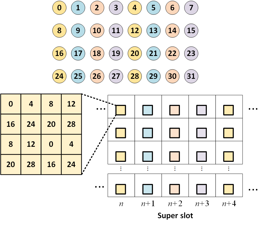
Fig. 2 shows the general architecture of the proposed framework. Firstly, we separate a whole array into , called division factor, non-overlapped and interleaved subarrays as shown in Fig. 3 and let UEs to estimate pilot CSIs of the subarrays and do interpolation for payload CSI acquisition. We term the pilot and payload CSI as partial CSI collectively. Secondly, an IDFT reformulation pre-processing is applied to partial CSIs for representations with higher sparsity and the combination at the gNB. Then, UEs encode them in every super slots and feedback to the gNB for partial CSI recovery. Subsequently, with the aids of high temporal correlation, a combining network is designed to merge the partial CSIs received in the most recent super slots for full CSI recovery. In this section, the above are described in details as follows:

III-A IDFT reformulation pre-processing
To maintain the efficiency to encode CSIs, most of the state-of-the-art works [1, 4, 8] opt to compress DA domain CSIs at UE side since they are with sparser representations. By reformulating the full CSI, we can decompose the DA domain full CSI as the summation of the independent partial DA domain CSIs ,…, as follows:
| (6) |
| (7) |
where denotes the CSI in delay-spatial (DS) domain and we can find that the partial DA domain CSIs are periodic with a constant phase difference and a period of elements along with the angle axis22 2 The details of the derivation is described in Appendix. as shown as follows:
| (8) |
denotes the -th column of a matrix . We denote the truncated matrices of partial CSIs ,…, as ,…, in this paper for brevity. In Eq. 8, given the characteristic of the spatially down-sampled subarrays, we can find that only the first columns of the truncated matrices ,…, are aperiodic and the remaining are simply their copies with constant phase rotations. Hence, UEs only need to encode the non-periodic portion of the matrices, ,…,, with a size of , whose size is reduced by a factor of as compared to the full CSI.
III-B STNet
We now present a new DLN called STNet. For recovering the CSI of the -th super slot, gNB decodes codewords received in the current and the previous super slots as estimated partial CSIs, and combine them as follows:
| (9) |
| (10) |
| (11) |
where , and denote encoding, decoding, and combining networks, respectively. is the non-periodic portion of the partial DL CSI transmitted by the UE in the -th super slot. denotes the remainder of a division of by . Before forwarding to the combining network, due to the periodic features of the partial CSIs, by following Eq. 10, rotation and concatenation operations are applied to the recovered partial CSIs , for initial estimation of the full CSI. Subsequently, it is forwarded to the combining network for the full CSI refinement and estimation.
As for the encoder network, similar to [5], we forward the real and imaginary parts of CSI to the encoder network, including four circular convolutional layers with 16, 8, 4, and 2 channels and activation functions. Given the circular characteristic of CSI matrices, we introduce circular convolutional layers to replace the traditional linear ones. Subsequently, a fully connected (FC) layer with elements is included for dimension reduction after reshaping. CR denotes the compression ratio. The output of the FC layer is then fed into the quantization module, called the sum-of-sigmoid (SSQ) [5] to generate codewords for feedback.
As for the decoder networks, similar to the encoder, we forward the received codewords to a FC layer with elements. Then, four circular convolutional layers with 16, 8, 4, and 2 channels and activation functions are included for partial CSI recovering. Then, the gNB forwards the current recovered partial CSI and the previous estimated partial CSIs to the combining network for final estimation. The combining network adopts the same design of the circular convolutional layers and activation functions as the decoder.
The STNet is optimized by updating the network parameters , and
| (12) |
where is the true DL CSI of the -th super slot.
Owing to the framework design, the required storage and computational complexity can be reduced significantly. In details, given the similar features of partial CSIs, only one encoder network needs to be trained and deployed at UEs. Plus, owing to the small input size for partial CSI compression, with the same compression ratio (CR)33 3 , the model parameters are reduced with a factor of as compared to the vanilla CsiNet Pro [7]. In addition, for recovery of the -th full CSI, although STNet collects the partial CSIs in the most recent super slots, with the locally available previous partial CSIs, only an additional process to encode and decode the partial CSI in the current super slot is required. Thus, the required UE storage and computational complexity can be significantly reduced44 4 Storage utilization is especially vital for UEs, as compared to gNBs. Note that, the selection of the division factor would significantly affect the recovery performance55 5 An excessive may induce recovery performance degradation since the recovered past partial CSIs could be uncorrelated to the current CSI., which will be demonstrated in Section IV.
IV Experimental Evaluations
IV-A Experiment Setup
In our experiments, we let the UL and DL bandwidths be 20 MHz and the subcarrier number be = 1024. We assume that the FDD system would place CSI-RS every time slots (i.e., ms). We consider both indoor and outdoor cases. We place the gNB with a height of 20 m at the center of a circular cell coverage with a radius of 20 m for indoor and 200 m for outdoor. We consider a gNB with a -element uniform linear array (ULA) communicates with UE with a single antenna. A half-wavelength inter-antenna spacing is considered. For each trained model, the number of epochs and batch size were set to 1,000 and 200, respectively. We generate several indoor and outdoor datasets, each containing 100,000 random channels. 60,000 and 20,000 random channels are for training and validation. The remaining 20,000 random channels are test data for performance evaluation.
For indoor data generation, we used the COST 2100 [10] simulator and select the scenario IndoorHall at 5GHz to generate indoor channels at 5.1-GHz UL and 5.3-GHz DL with LOS paths. The antenna and band types are set as MIMO VLA omni and wideband, respectively. As for the outdoor dataset, we utilized QuaDRiGa simulator [11] with the scenario features of 3GPP 38.901 UMa. We considered the UMa LOS and NLOS scenarios at 300 and 330 MHz of UL and DL bands, respectively, with different UE velocities (considering 1, 2 and 4 m/s). The antenna type is set to omni.
The performance metric is the normalized MSE
| (13) |
where the number and subscript denote the total number and index of channel realizations, respectively. Instead of evaluating the estimated DL CSI matrix , we evaluate the estimated SF-CSI matrix that can be obtained by reversing the Fourier processing and padding zero matrix. Note that this NMSE includes both the errors caused by truncation at the encoder and the overall recovery error. Thus, it is practically more meaningful.
In the following section, we evaluate the performance of CSI recovery by adopting the proposed partial CSI feedback framework. To show the efficacy of the framework, we compare the STNet with CsiNet Pro used in [7] which shares the same core layer design of the encoder/decoder networks. Namely, the CsiNet Pro can be regarded as the STNet without multiple super-slot branches and the combing network. As shown in Fig. 4, the only difference between STNet and CsiNet Pro is the IDFT reformulation pre-processing and the additional combining network.
As mentioned in Section III, STNet can obtain the current full CSI by obtaining the current partial CSI. Thus, in each super slot, as compared to CsiNet Pro, the codeword size to be transmitted at the same CR can be reduced by a factor of . Herein we define a new term called effective compression ratio ().

IV-B Different Division Factor
To demonstrate the superiority of the proposed framework, we first applied different division factors in both indoor and outdoor scenarios with low UE mobility (m/s) for different effective compression ratios . Fig. 5 (a), (b) and (c) show the NMSE performance of the proposed framework STNet and vanilla CsiNet Pro under indoor and outdoor scenarios, respectively, at different compression ratios. By adopting the proposed framework, with the aids of the high CSI temporal correlation, STNet performs much better than CsiNet Pro and has the best performance when using a larger division factor . However, for higher recovery accuracy, we still cannot just choose a large division factor in all scenarios, especially in outdoor scenarios since STNet highly depends on the CSI temporal correlation. The reason will be shown in the following section.

IV-C Different UE mobility
To comprehensively assess the robustness of the proposed framework, we tested the same alternatives in outdoor scenarios with different UE mobility (= 1, 2 , 4 m/s66 6 These velocities roughly corresponds to the UE velocities of walking, jogging, and biking, respectively.). Fig. 6 shows the NMSE performance of STNet and CsiNet Pro in the outdoor scenarios with different average UE velocity and at different compression ratios. We can find that STNet performance degrades as the increasing UE velocity and even perform worse than CsiNet Pro when division factor . Namely, the higher UE mobility would induce a lower CSI temporal correlation, causing the performance degradation of STNet. According to the numerical simulations, to strike a trade-off, an intermediate division factor seems to be a plausible solution in outdoor scenarios.

IV-D Assessment of FLOPs and parameter numbers
| FLOPs | Parameters | |||
|---|---|---|---|---|
| Method | ||||
| STNet, | 1.1M | 583K | 555K | 292K |
| STNet, | 583K | 321K | 292K | 160K |
| CsiNet Pro | 2.13M | 1.08M | 1.07M | 0.54M |
Due to the limited storage and computation power of UEs, it is crucial to design a light-weighted and easy-to-implement neural network. Table I shows that, besides the superiority in terms of the NMSE performance, the required computation power and storage for model parameters can also significantly reduced. To explain, with smaller input and output sizes of STNet’s encoder and decoder networks, the required FLOPs and parameters are significantly lower than CsiNet Pro. In addition, since STNet can act in a sliding window fashion, the encoder and decoder networks are conducted only once instead of times. Thus, even considering the implementation of the combing network, the STNet’s FLOPs and parameters are still obviously less than the ones of CsiNet Pro.
V Conclusions
This work presents a new deep learning framework for large scale CSI estimation that utilizes partial CSI feedback compression and leverages CSI temporal correlation in FDD systems. To control time-frequency resources needed for CSI-RS in the proposed IDFT reformulation, our proposed STNet allows UE to transmit partial CSI feedbacks associated with interleaved non-overlapped subarrays in super slots. Subsequently, the gNB estimates the full CSI based on aggregated partial feedbacks by utilizing CSI temporal correlation. Our test results demonstrate significant improvement of recovery performance at reduced computation complexity and storage usage in comparison with the existing benchmark model of CsiNet Pro.
Appendix
Proof of Eq. (8):
Since the array is divided into non-overlapped and interleaved subarrays, the CSI matrix in DS and DA domains for the -th subarray are expressed respectively as follows:
| (A.1) |
| (A.2) | ||||
By substituting the column index by , we can find that the CSI matrix in DA domain is periodic with a constant phase difference and a period of elements along with the angle axis as follows:
| (A.3) | ||||
where
| (A.4) |
| (A.5) |
References
- [1] C. Wen, W. Shih, and S. Jin, “Deep Learning for Massive MIMO CSI Feedback,” IEEE Wirel. Commun. Lett., vol. 7, no. 5, pp. 748–751, 2018.
- [2] J. Guo et al., “Convolutional Neural Network-Based Multiple-Rate Compressive Sensing for Massive MIMO CSI Feedback: Design, Simulation, and Analysis,” IEEE Trans. Wirel. Commun., vol. 19, no. 4, pp. 2827–2840, 2020.
- [3] Z. Qin et al., “Deep Learning in Physical Layer Communications,” IEEE Wirel. Commun., vol. 26, no. 2, pp. 93–99, 2019.
- [4] Z. Liu, L. Zhang, and Z. Ding, “Exploiting Bi-Directional Channel Reciprocity in Deep Learning for Low Rate Massive MIMO CSI Feedback,” IEEE Wirel. Commun. Lett., vol. 8, no. 3, pp. 889–892, 2019.
- [5] ——, “An Efficient Deep Learning Framework for Low Rate Massive MIMO CSI Reporting,” IEEE Trans. Commun., vol. 68, no. 8, pp. 4761–4772, 2020.
- [6] Y.-C. Lin, Z. Liu, T.-S. Lee, and Z. Ding, “Deep Learning Phase Compression for MIMO CSI Feedback by Exploiting FDD Channel Reciprocity,” IEEE Wireless Commun. Lett., pp. 1–1, 2021, early access.
- [7] Z. Liu, M. Rosario, and Z. Ding, “A Markovian Model-Driven Deep Learning Framework for Massive MIMO CSI Feedback,” arXiv preprint arXiv:2009.09468, 2020.
- [8] J. Guo et al., “DL-based CSI Feedback and Cooperative Recovery in Massive MIMO,” arXiv preprint arXiv:2003.03303, 2020.
- [9] 3GPP, “NR; Physical Channels and Modulation,” 3rd Generation Partnership Project (3GPP), Technical Specification (TS) 38.211, June 2020, version 16.6.0.
- [10] L. Liu et al., “The COST 2100 MIMO Channel Model,” IEEE Wirel. Commun., vol. 19, no. 6, pp. 92–99, 2012.
- [11] S. Jaeckel et al., “QuaDRiGa: A 3-D Multi-Cell Channel Model with Time Evolution for Enabling Virtual Field Trials,” IEEE Trans. Antennas and Propag., vol. 62, no. 6, pp. 3242–3256, 2014.