Bifurcations of a neural network model with symmetry

Today experimental techniques allow an increasingly detailed view of the physical architecture of biological neural networks. However, drawing a clear line from physical connectivity to dynamic neural activity is still a challenge. The networks in question are massive in scale and high dimensional (with billions of neurons and possibly trillions of synapse). Neural networks also show great diversity in structure at every level, from the morphology and excitability properties of a single cell to large scale connections between brain regions.

One common experimental finding is that neural dynamics are surprisingly low-dimensional when compared to the overall dimensionality of the neural system [17, 8, 19, 42, 30] (see Fig. 1 of [21] for a summary of earlier studies). The low-dimensional manifold may even shift slowly over time, as the underlying components of the network (cells and synapses) die and are replaced [20]. Thus, a major challenge for modern mathematical neuroscience is to understand how low-dimensional dynamics emerges from the observed connectivity of the brain.

Real neural networks are partially structured but also partially random. Intuitively, it’s clear that not every connection in the brain must be tuned precisely (after all, every person reading this sentence will respond to these black markings in the same way, despite significant differences between our individual brains). This has motivated the use of analytical tools of random network theory, in which one seeks to draw conclusions about an ensemble of networks. An early example is the work by Sompolinsky et al. [40] which applies dynamic mean field theory to single-population firing-rate networks in which connections are chosen from a mean-zero Gaussian distribution: in the limit of large network size, the authors find that the network transitions from quiescence to chaos as a global coupling parameter passes a bifurcation value. This value coincides with the point at which the spectrum of the connectivity matrix exits the unit circle [23, 3] thus making the connection to random matrix theory very concrete. Later authors have sought to extend these results to correlated or block-structured matrices [31, 2], and many others have studied the spectral characteristics of partially structured connection matrices [43, 1, 35] with neural networks as a primary motivation.

However, the results of spectral theory and nonlinear dynamics have not always neatly aligned. One network setting that has caused persistent difficulty is excitatory-inhibitory networks with strong average connections [36]. The predictions of random matrix theory suggest chaotic, asynchronous fluctuations, whereas large-scale coherent fluctuations have been observed instead. Why? The answer may be found in the nature of the deterministic perturbation. Several authors have examined how low-rank, asymmetric perturbations create an effectively feed-forward structure that allows coherent dynamics to co-exist with random fluctuations in an orthogonal subspace [14, 13, 33, 32]; the dimensionality of the dynamical subspace can be related to the dimension of the low-rank perturbation in the connectivity matrix [39, 5].

In an earlier work, we found an alternative possibility [4]. In examining balanced E-I networks without self-coupling, we persistently observed periodic solutions which could not be explained by random matrix theory. Instead, they arose as a consequence of underlying symmetries in the connection matrix and could be predicted through the machinery of equivariant bifurcation theory. However, some pieces of our analysis remained uncompleted: we were unable at that time to give a complete stability analysis. This is important because the stable solution is what one can expect to observe in a perturbed (random) network.

Here, we complete this analysis for all-to-all excitatory-inhibitory networks. We then extend this analysis to a biologically significant block-structured case, in which the excitatory cells are clustered, but inhibition is global. We find that the dynamics are strikingly different: instead of limit cycles, we predict fixed points. In both cases, the structures can be understood by considering the symmetries of the deterministic connection matrix.

We consider a network in which each node represents the firing rate of a single neuron. The individual neurons are connected by sigmoidal activation functions through a connectivity matrix, which specifies both the network of neuronal connections and the weight of each connection, including whether a given neuron is excitatory (E) or inhibitory (I). With noise in the connectivity matrix, this is an idealized model in neuroscience [22, 36, 31]. Here, we will consider the system without noise, but where the connection weights have important symmetries. Specifically, we study:

for $\mathbf{x}\in\mathbb{R}^{N}$, where the global coupling strength, $g$, is used a bifurcation parameter. The network comprises a total of $N$ neurons, of which $n_{E}$ are excitatory and $n_{I}$ are inhibitory. $H$ is the $N\times N$ connectivity matrix; the diagonal entries of $H$ are all 0 to exclude self-interactions of neurons (see [4, Sec. 2.1] for a discussion on why self-coupling of neurons is removed). We will use the parameter $f=n_{E}/N$ to identify the fraction of neurons that are excitatory: for the remainder of this paper we will use $f=0.8$ for a 4-to-1 excitatory-to-inhibitory ratio, which is typical for cortical networks [7]. We note that $F$ is an odd function of $\mathbf{x}$, i.e. $F(-\mathbf{x})=-F(\mathbf{x})$. This implies that if $\mathbf{x}(t)$ is a solution to eq. 1, so is $-\mathbf{x}(t)$, and that $\mathbf{x}=\mathbf{0}$ is a fixed point of eq. 1 for all $g$.

We consider here networks in which the excitatory neurons are grouped into $n_{C}$ clusters, each containing $p$ neurons, and the inhibitory neurons are grouped into $n_{C_{I}}$ clusters, each containing $p_{I}$ neurons. For simplicity, we only consider the case where the excitatory clusters are the same size, and the inhibitory clusters are the same size. This restriction introduces additional symmetries into the model, which are explained below. In addition, all connections of any given type (e.g. $E\rightarrow E$ or $E\rightarrow I$) will have the same strength. The matrix $H$ then takes the general form

where $\mathbf{1}_{m\times n}$ is the $m\times n$ matrix of ones, and $\mathbf{K}_{n}$ is the $n\times n$ matrix with all ones off the diagonal, i.e. $\mathbf{K}_{n}=\mathbf{1}_{n\times 1}\left(\mathbf{1}_{n\times 1}\right)^{T}-\mathbf{I}_{n}$, with $\mathbf{I}_{n}$ the $n\times n$ identity matrix. The connection weights $\mu$ are defined “matrix-style”, e.g. $\mu_{EI}$ will denote the connection from I to E, while $\mu_{IE}$ will denote the connection from E to I. The weights are also signed, so that $\mu_{EE},\mu_{IE}>0$ and $\mu_{EI},\mu_{II}<0$: this reflects the neurobiological heuristic of Dale’s Law, which states that each neuron makes excitatory or inhibitory connections onto its postsynaptic targets.

The model eq. 1, eq. 2 is equivariant under the subgroup $\Gamma_{H}$ of $S_{N}$, defined by

where $S_{n}$ is the group of permutations on $n$ objects (see section 3 for the definition of equivariance). Essentially, this says that labels of the neurons within each cluster can be freely permuted. Since the clusters are of equal sizes, there are two additional symmetries in the model. The labels of the excitatory clusters and the labels of the inhibitory clusters can be freely permuted, yielding symmetry groups isomorphic to $S_{n_{C}}$ and $S_{n_{C_{I}}}$, respectively.

The linearization of eq. 1 about $\mathbf{x}=0$ is the matrix

where $I_{N}$ is the $N\times N$ identity matrix. The eigenvalues of $DF(0)$ are then given by $\lambda^{*}(g)=\frac{g}{\sqrt{N}}\lambda-1$ for all eigenvalues $\lambda$ of $H$. As a consequence, the dynamics of the system can be understood in terms of the eigenvalues of $H$. For an eigenvalue $\lambda$ of $H$ with negative real part, the corresponding eigenvalue $\lambda^{*}(g)$ of $DF(0)$ will always have negative real part, irrespective of $g$. On the other hand, for an eigenvalue $\lambda$ of $H$ with positive real part, the sign of the real part of the corresponding eigenvalue $\lambda^{*}(g)$ of $DF(0)$ will depend on the bifurcation parameter $g$. Thus, the only bifurcations of $\mathbf{x}=0$ involve the eigenvalues of $H$ which have positive real part. Furthermore, the multiplicities of the eigenvalues of $H$ are determined by symmetries in the underlying model eq. 1 and the matrix $H$. These lead to symmetric bifurcations as $g$ is varied; we address this in §3.

The dynamics near a nonzero fixed point $\mathbf{x}^{*}=(x_{1}^{*},\dots,x_{N}^{*})^{T}$ of eq. 1 also depend on the matrix $H$. The linearization of eq. 1 about $\mathbf{x}^{*}$ is the matrix

where

is obtained from the matrix $H$ by multiplying column $j$ of $H$ by $\sech^{2}(gx_{j}^{*})$. We note that the diagonal entries of $H(\mathbf{x}^{*})$ are 0, thus $\text{Trace }H(\mathbf{x}^{*})=0$. This implies that the eigenvalues of $H(\mathbf{x}^{*})$ sum to 0.

We first studied this system in [4], where we analyzed all-to-all connected, balanced excitatory-inhibitory networks ($n_{C}=1$ and $n_{C_{I}}=1$). In this paper, we first flesh out some details about that system: we derive leading order expressions for bifurcation points in the system, for the equilibria near those bifurcation points, and for the Hopf bifurcations that spawn the clustered limit cycles we observed in [4] (section 5). We then extend the analysis to networks in which the excitatory population is split up into clusters ($n_{C}>1$ and $n_{C_{I}}=1$; section 6). We briefly compare with networks in which the inhibitory neurons are clustered instead ($n_{C}=1,n_{C_{I}}>1$; section 7).

In this section, we outline the tools of equivariant bifurcation theory, and explain how they apply to the model in question. Our main tool for analyzing the solutions to eq. 1, eq. 2 which arise at bifurcation points when symmetries are present is the Equivariant Branching Lemma [24, 10, 25, 28]. Before stating the result, we introduce some terminology.

Let $\Gamma$ be a finite group acting on $\mathbb{R}^{N}$; then we say that a mapping $F:\mathbb{R}^{N}\rightarrow\mathbb{R}^{N}$ is $\Gamma$-equivariant if $F(\gamma\mathbf{x})=\gamma F(\mathbf{x})$, for all $\mathbf{x}\in\mathbb{R}^{N}$ and $\gamma\in\Gamma$. A one-parameter family of mappings $F:\mathbb{R}^{N}\times\mathbb{R}\rightarrow\mathbb{R}^{N}$ is $\Gamma$-equivariant, if it is $\Gamma$-equivariant for each value of its second argument. We say that $V$, a subspace of $\mathbb{R}^{N}$, is $\Gamma$-invariant if $\gamma\mathbf{v}\in V$, for any $\mathbf{v}\in V$ and $\gamma\in\Gamma$. We furthermore say that the action of $\Gamma$ on $V$ is irreducible if $V$ has no proper invariant subspaces, i.e. the only $\Gamma$-invariant subspaces of $V$ are $\{0\}$ and $V$ itself.

For a group $\Gamma$ and a vector space $V$, we define the fixed-point subspace for $\Gamma$, denoted ${\rm Fix}_{V}(\Gamma)$, to be all points in $V$ that are unchanged under any of the members of $\Gamma$, i.e. ${\rm Fix}_{V}(\Gamma)=\{\mathbf{x}\in V:\gamma\mathbf{x}=\mathbf{x},\forall\gamma\in\Gamma\}$. The isotropy subgroup of $\mathbf{x}\in V$, denoted $\Sigma_{x}$, is the set of all members of $\Gamma$ under which $\mathbf{x}$ is fixed, i.e. $\Sigma_{x}=\{\gamma\in\Gamma:\gamma\mathbf{x}=\mathbf{x}\}$. We then say that a subgroup $\Sigma$ is an isotropy subgroup of $\Gamma$, if it is the isotropy subgroup, $\Sigma_{x}$, for some $\mathbf{x}\in V$.

Suppose we have a one-parameter family of mappings, $F(\mathbf{x},g)$, and we wish to solve $F(\mathbf{x},g)=0$. For any $(\mathbf{x},g)\in\mathbb{R}^{n}\times\mathbb{R}$, let $(DF)_{\mathbf{x},g}$ denote the $N\times N$ Jacobian matrix

A bifurcation will occur when the Jacobian ceases to be invertible, i.e. when $(DF)_{\mathbf{x},g}$ has a nontrivial kernel. For a $\Gamma$-equivariant mapping — i.e. $F(\mathbf{x},g)$ is $\Gamma$-equivariant for any value of the parameter $g$ — we may have multiple eigenvalues go through zero at once, because of symmetries; however, some of the structural changes that occur are qualitatively the same as those that occur in a non-symmetric system in which a single eigenvalue crosses through zero. But there is a catch: we will have multiple such solution branches, each corresponding to a subgroup of the original symmetries. This is formalized in the following theorem:

As we have noted, eq. 1, eq. 2 is $\Gamma_{H}$-equivariant, where

and $S_{n}$ is the group of permutations on $n$ objects. Essentially, this says that labels of the neurons within each cluster can be freely permuted. In addition, the labels of the excitatory clusters and the labels of the inhibitory clusters can be freely permuted, yielding symmetry groups isomorphic to $S_{n_{C}}$ and $S_{n_{C_{I}}}$, respectively.

The origin, $\mathbf{x}=\mathbf{0}$ is a fixed point for all values of $g$. As we increase $g$ from 0, we will encounter a sequence of bifurcation points, i.e. points $(\mathbf{x}_{0},g_{0})$ for which $DF$ has a nontrivial kernel. At each such point, we will identify the kernel $V$ and the subgroups $\Sigma$ for which a solution is guaranteed by the Equivariant Branching Lemma.

We can simplify the model using the fact that all cells within each excitatory cluster must be synchronized at a fixed point or periodic orbit. In the case where there is a single excitatory cluster ($n_{C}=1$), if $x_{1}$ and $x_{2}$ are the activities of two excitatory cells, then a straightforward calculation (see Lemma 3 from [4]) shows that

The only way this can be true for a fixed point (for which $\frac{d}{dt}|x_{1}-x_{2}|^{2}=0$) or for a periodic orbit (for which $x_{1}(t)-x_{2}(t)=x_{1}(t+T)-x_{2}(t+T)$ for some period $T$) is if $x_{1}(t)=x_{2}(t)$ for all $t$. If $n_{C}>1$, and $x_{1}$ and $x_{2}$ are the activities of two cells in the same excitatory cluster, equation eq. 7 holds by the same argument as in [4], since both neurons receive the same incoming connections with the same weights.

We are primarily interested in the case where there is a single cluster of inhibitory cells, i.e. $n_{C_{I}}=1$. (We will briefly consider the case of multiple inhibitory clusters in section 7). If there are $n_{C}$ excitatory clusters containing $p$ cells each, and $n_{I}$ inhibitory cells (for $N=pn_{C}+n_{I}$ total cells), equation eq. 1 reduces to the system of $n_{C}+n_{I}$ equations

where $x_{E_{j}}$ is the activity for the $j$th excitatory cluster, and $x_{I_{j}}$ is activity for the $j$th inhibitory cell. In matrix form, the equations eq. 8 can be written

where $\mathbf{x}=(x_{E_{1}},\dots,x_{E_{n_{C}}},x_{I_{1}},\dots,x_{I_{n_{I}}})^{T}$, and $\tilde{H}$ is the $(n_{C}+n_{I})\times(n_{C}+n_{I})$ reduced matrix

The system of equations eq. 9, eq. 10 is the restriction of the original system eq. 1, eq. 2 with $n_{C_{I}}=1$ to the fixed-point subspace ${\rm Fix}(\Gamma_{C})$ corresponding to the subgroup

of $\Gamma_{H}$, where $E_{n_{I}}$ is the trivial subgroup of $S_{n_{I}}$ consisting only of the identity permutation. The reduced model eq. 9, eq. 10 is then equivariant under the subgroup

of $S_{n_{C}+n_{I}}$. The special case of $n_{C}=1$ (a single excitatory cluster), for which $\Gamma=S_{1}\times S_{n_{I}}$, is considered in section 5. We note that in this case, one of the symmetries is effectively lost, since the activity of the lone excitatory cluster is represented by a single variable. The general case ($n_{C}>1$) is considered in section 6. We will only consider the reduced system eq. 9, eq. 10 in section 5 and section 6.

Next, we show that no stability information is lost by only studying the reduced system. Suppose $\mathbf{x}^{*}=(x_{E_{1}}^{*},\dots,x_{E_{n_{C}}}^{*},x_{I_{1}}^{*},\dots,x_{I_{n_{I}}}^{*})^{T}$ is a fixed point of eq. 9. (We will discuss the existence of such fixed points in section 5 and section 6). The linearization of eq. 9 about $\mathbf{x}^{*}$ is the matrix

where

The original system eq. 1 has a corresponding fixed point $\mathbf{x}_{0}^{*}$, in which each $x_{E_{j}}^{*}$ in $\mathbf{x}^{*}$ is repeated $p$ times. The following proposition shows that to analyze the stability of the fixed point $\mathbf{x}_{0}^{*}$ in the full system eq. 1, it suffices to determine the eigenvalues of the reduced matrix $\tilde{H}(\mathbf{x}^{*})$, since the additional eigenvalues of $H(\mathbf{x}_{0}^{*})$ are negative, and thus will not affect stability.

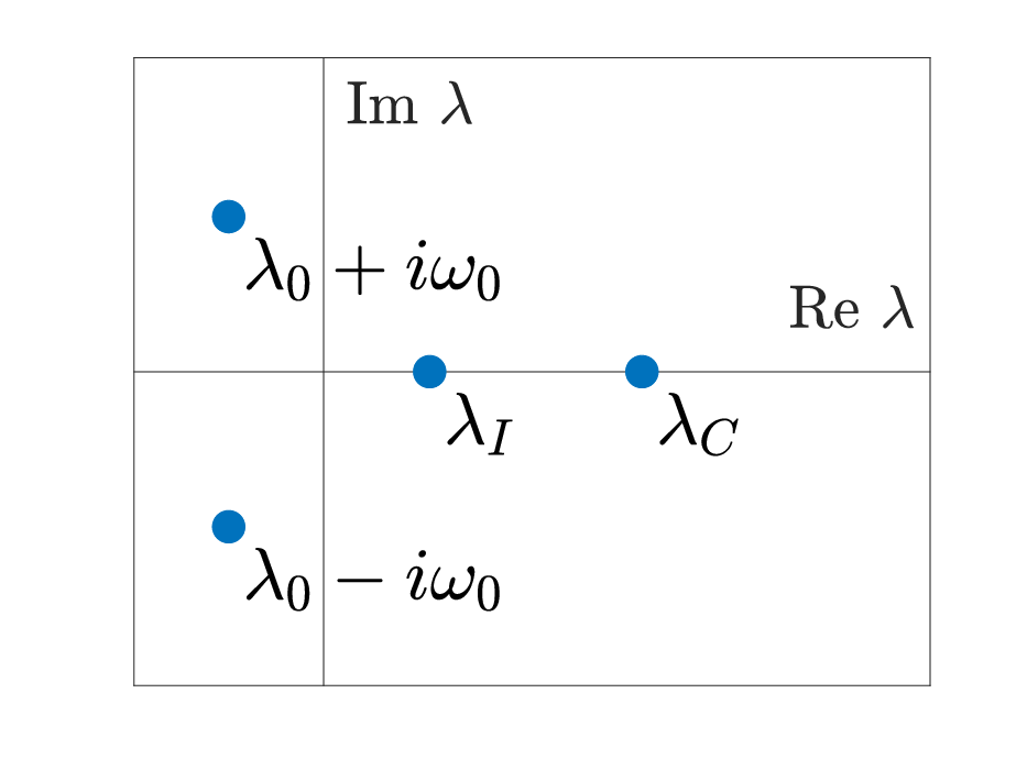
The dynamics of the full system can therefore be explained by the dynamics of the reduced system, and, in particular, in terms of the eigenvalues of the reduced matrix $\tilde{H}$ (fig. 1). Although these patterns will be explained in detail in the corresponding sections below, we point out two crucial differences between the model with a single excitatory cluster (fig. 1, left) and the model with multiple excitatory clusters (fig. 1, right). For the model with multiple excitatory clusters, there is an additional positive, real eigenvalue $\lambda_{C}$, and the complex pair $\lambda_{0}+i\omega_{0}$ has negative real part.

The simplest case (considered in [4]) involves a single excitatory cluster ($n_{C}=1$ and $p=n_{E}$) and a single inhibitory cluster, in which case the matrix $\tilde{H}$ in eq. 9 reduces to the $(1+n_{I})\times(1+n_{I})$ matrix

We choose the connection weights so that the network is balanced; that is, the excitatory and inhibitory currents coming into each cell should approximately cancel [36]. To achieve this balance, we set $\mu_{EI}=-\alpha\mu_{EE}$ and $\mu_{II}=-\alpha\mu_{IE}$, where $\alpha=\frac{f}{1-f}$. For simplicity, we also take $\mu_{IE}=\mu_{EE}$. The spectrum of $\tilde{H}$ is now easy to compute (see [4], noting that the full matrix $H$ is considered in that work). The eigenvalues of $\tilde{H}$ (left panel of fig. 1) are

• •

  $\lambda_{I}:=\alpha\mu_{EE}>0$ with multiplicity $n_{I}-1$.

• •

  One complex pair of eigenvalues $\lambda_{0}\pm i\omega_{0}$, with

  $$\lambda_{0}:=\mu_{EE}\frac{\alpha-1}{2},\quad\omega_{0}:=\mu_{EE}\sqrt{\alpha+1}\sqrt{n_{E}-\frac{\alpha+1}{4}}.$$

It is straightforward to check that $0<\lambda_{0}<\lambda_{I}$. Since both of these are positive, there will be a bifurcation of $\mathbf{x}=0$ involving each of these eigenvalues.

In the following sections, we will determine the bifurcations which occur as $g$ is increased, together with the structures which emerge at these bifurcation points. First, the origin loses stability in a symmetric pitchfork bifurcation, after which point there is a branch of equilibria for every possible division of the inhibitory cells into two groups. We will derive leading order formulas for these branches, as well as show which of them are initially stable. As $g$ is further increased, there is a Hopf bifurcation on each of these branches, which gives rise to a limit cycle with the same grouping pattern as the corresponding branch. Finally, at a critical value of $g$, these limit cycles coalesce into a symmetric pitchfork bifurcation of limit cycles. After this point, there is a single stable limit cycle in which there is one group of inhibitory cells and one group of excitatory cells.

References

- [1] Y. Ahmadian, F. Fumarola, and K. D. Miller, Properties of networks with partially structured and partially random connectivity, Physical Review E, 91 (2015), p. 012820.
- [2] J. Aljadeff, M. Stern, and T. Sharpee, Transition to chaos in random networks with cell-type-specific connectivity, Physical Review Letters, 114 (2015), p. 088101.
- [3] Z. Bai, Circular law, Annals of Probability, 25 (1997), pp. 494–529.
- [4] A. K. Barreiro, Kutz, J. Nathan, and Shlizerman, Eli, Symmetries Constrain Dynamics in a Family of Balanced Neural Networks, Journal of Mathematical Neuroscience, 7 (2017), p. 28, https://doi.org/10.1186/s13408-017-0052-6.
- [5] M. Beiran, A. Dubreuil, A. Valente, F. Mastrogiuseppe, and S. Ostojic, Shaping dynamics with multiple populations in low-rank recurrent networks, Neural Computation, 33 (2021), pp. 1572–1615.
- [6] N. Brunal and V. Hakim, Fast global oscillations in networks of integrate-and-fire neurons with low firing rates, Neural Computation, 11 (1999), pp. 1621–1671.
- [7] D. Buxhoeveden and M. Casanova, The minicolumn hypothesis in neuroscience, Brain, 125 (2002), pp. 935–951.
- [8] W. Chaisangmongkon, S. K. Swaminathan, D. J. Freedman, and X. J. Wang, Computing by robust transience: How the fronto-parietal network performs sequential, category-based decisions, Neuron, 93 (2017), pp. 1504–1517.
- [9] C. C. Chow and Y. Karimipanah, Before and beyond the wilson-cowan equations, Journal of neurophysiology, 123 (2020), pp. 1645–1656, https://doi.org/10.1152/jn.00404.2019.
- [10] G. Cicogna, Symmetry breakdown from bifurcation, Lett. Nuovo Cimento (2), 31 (1981), pp. 600–602.
- [11] E. A. Coddington and N. Levinson, Theory of ordinary differential equations, McGraw-Hill New York, 1955.
- [12] D. Dahmen, S. Recanatesi, X. Jia, G. K. Ocker, L. Campagnola, T. Jarsky, S. Seeman, M. Helias, and E. Shea-Brown, Strong and localized coupling controls dimensionality of neural activity across brain areas, bioRxiv, (2021), pp. 2020–11.
- [13] R. Darshan, C. V. Vreeswijk, and D. Hansel, Strength of correlations in strongly recurrent neuronal networks, Phys. Rev. X, 8 (2018).
- [14] L. G. del Molino, K. Pakdaman, J. Touboul, and G. Wainrib, Synchronization in random balanced networks, Physical Review E, 88 (2013), p. 042824.
- [15] E. J. Doedel, T. F. Fairgrieve, B. Sandstede, A. R. Champneys, Y. A. Kuznetsov, and X. Wang, AUTO-07P: Continuation and bifurcation software for ordinary differential equations, tech. report, 2007.
- [16] C. Ebsch and R. Rosenbaum, Imbalanced amplification: A mechanism of amplification and suppression from local imbalance of excitation and inhibition in cortical circuits, PLoS computational biology, 14 (2018), p. e1006048.
- [17] A. Ecker, P. Berens, R. J. Cotton, M. Subramaniyan, G. H. Denfield, C. R. Cadwell, S. M. Smirnakis, M. Bethge, and A. S. Tolias, State dependence of noise correlations in macaque primary visual cortex, Neuron, 82 (2014), pp. 235–248.
- [18] G. Ermentrout and D. Terman, Foundations of Mathematical Neuroscience, Springer, 2010.
- [19] J. A. Gallego, P. M. G., S. N. Naufel, C. Ethier, S. A. Solla, and L. E. Miller, Cortical population activity within a preserved neural manifold underlies multiple motor behaviors, Nature Communications, 9 (2018), pp. 1–13.
- [20] J. A. Gallego, M. G. Perich, R. H. Chowdhury, S. A. Solla, and L. E. Miller, Long-term stability of cortical population dynamics underlying consistent behavior, Nature neuroscience, 23 (2020), pp. 260–270.
- [21] P. Gao, S. Ganguli, F. P. Battaglia, and M. J. Schnitzer, On simplicity and complexity in the brave new world of large-scale neuroscience, Current Opinion in Neurobiology, 32 (2015), pp. 148–155.
- [22] I. Ginzburg and H. Sompolinsky, Theory of correlations in stochastic neural networks, Physical Review E, 50 (1994), pp. 3171–3191.
- [23] V. Girko, Circular law, Theory Probab. Appl., 29 (1985), pp. 694–706.
- [24] M. Golubitsky and I. Stewart, The Symmetry Perspective, Birkhäuser Basel, 2002, https://doi.org/10.1007/978-3-0348-8167-8, https://doi.org/10.1007%2F978-3-0348-8167-8.
- [25] M. Golubitsky, I. Stewart, and D. Schaeffer, Singularities and Groups in Bifurcation Theory, Vol II, Springer-Verlag, 1988.
- [26] G. Hermann and J. Touboul, Heterogeneous connections induce oscillations in large-scale networks, Physical Review Letters, 109 (2012), p. 018702.
- [27] M. H. Holmes, Introduction to Perturbation Methods, Texts in Applied Mathematics, Springer, 2nd ed. 2013 ed., 2012.
- [28] R. B. Hoyle, Pattern formation : an introduction to methods, Cambridge texts in applied mathematics, Cambridge University, Cambridge, 2006.
- [29] Y. Hu, J. Trousdale, K. Josić, and E. Shea-Brown, Local paths to global coherence: Cutting networks down to size, Physical Review E, 89 (2014), p. 032802.
- [30] C. Huang, D. A. Ruff, R. Pyle, R. Rosenbaum, M. R. Cohen, and B. Doiron, Circuit models of low-dimensional shared variability in cortical networks, Neuron, 101 (2019), pp. 337–348.
- [31] J. Kadmon and H. Sompolinsky, Transition to chaos in random neuronal networks, Physical Review X, 5 (2015), p. 041030.
- [32] I. Landau and H. Sompolinsky, Macroscopic fluctuations emerge in balanced networks with incomplete recurrent alignment, Physical Review Research, 3 (2021).
- [33] I. D. Landau and H. Sompolinsky, Coherent chaos in a recurrent neural network with structured connectivity, PLoS Comput. Biol., 14 (2018).
- [34] D. Martí, N. Brunel, and S. Ostojic, Correlations between synapses in pairs of neurons slow down dynamics in randomly connected neural networks, Physical Review E, 97 (2018), p. 062314.
- [35] D. Muir and T. Mrsic-Flogel, Eigenspectrum bounds for semirandom matrices with modular and spatial structure for neural networks, Physical Review E, 91 (2015), p. 042808.
- [36] K. Rajan and L. Abbott, Eigenvalue spectra of random matrices for neural networks, Physical Review Letters, 97 (2006), p. 188104.
- [37] S. Recanatesi, G. K. Ocker, M. A. Buice, and E. Shea-Brown, Dimensionality in recurrent spiking networks: Global trends in activity and local origins in connectivity, PLoS computational biology, 15 (2019), p. e1006446.
- [38] R. Rosenbaum, M. A. Smith, A. Kohn, J. E. Rubin, and B. Doiron, The spatial structure of correlated neuronal variability, Nature Neuroscience, 20 (2017), pp. 107–114.
- [39] F. Schuessler, A. Dubreuil, F. Mastrogiuseppe, S. Ostojic, and O. Barak, Dynamics of random recurrent networks with correlated low-rank structure, Phys. Rev. Research, 2 (2020).
- [40] H. Sompolinsky, A. Crisanti, and H. Sommers, Chaos in random neural networks, Physical Review Letters, 61 (1988), pp. 259–262.
- [41] M. Stern, H. Sompolinsky, and L. F. Abbott, Dynamics of random neural networks with bistable units, Physical Review E, 90 (2014), p. 062710.
- [42] J. Wang, D. Narain, E. A. Hosseini, and M. Jazayeri, Flexible timing by temporal scaling of cortical responses, Nature Neuroscience, 21 (2018), pp. 102–112.
- [43] Y. Wei, Eigenvalue spectra of asymmetric random matrices for multicomponent neural networks, Physical Review E, 85 (2012), p. 066116.