Sensor Applications
Anomalous sensor detection, Principal component analysis, -kernel, multiplication-free method.
Detecting Anomaly in Chemical Sensors via L1-Kernel based Principal Component Analysis
Abstract
We propose a kernel-PCA based method to detect anomaly in chemical sensors. We use temporal signals produced by chemical sensors to form vectors to perform the Principal Component Analysis (PCA). We estimate the kernel-covariance matrix of the sensor data and compute the eigenvector corresponding to the largest eigenvalue of the covariance matrix. The anomaly can be detected by comparing the difference between the actual sensor data and the reconstructed data from the dominant eigenvector. In this paper, we introduce a new multiplication-free kernel, which is related to the -norm for the anomaly detection task. The -kernel PCA is not only computationally efficient but also energy-efficient because it does not require any actual multiplications during the kernel covariance matrix computation. Our experimental results show that our kernel-PCA method achieves a higher area under curvature (AUC) score (0.7483) than the baseline regular PCA method (0.7366).
1 Introduction
Chemical sensors are widely used to detect ammonia, methane, and other Volatile Organic Compounds (VOCs) [1, 2, 3]. The life and performance of chemical gas detection sensors can be affected by various factors, including temperature, humidity, other interfering chemical gases, physical factors etc. Anomalous sensors can produce drifting waveforms and it is a fatal problem for reliable gas identification and concentration estimation [4, 5]. In this work, we determine anomalous sensors and sensor measurements in an array of uncalibrated sensors by using robust -Principal Component Analysis (PCA) without using a reference time-series data.
PCA is used in anomalous sensor and sensor signal detection [6, 7, 8]. In this approach, the covariance matrix is constructed from a set of data vectors and the anomalous items (outliers) or vectors are found by using the reconstruction difference [9, 10]. The principal components of the data covariance matrix is computed and the original data vectors are reconstructed using only the first few principal components. In general, the reconstructed data vector is similar to the original data vectors, and the reconstructed data items that are different from the corresponding original items are considered to be anomalous.
In this paper, we propose to use -kernel PCA based on a multiplication-free kernel to detect anomaly in chemical sensors. Although the conventional PCA, which is based on the -norm has successfully solved many problems it is sensitive to outliers in the data because the effects of the outliers are over-amplified by the -norm. Recently, it has been shown that -norm based methods produce better results in practical problems compared to the -norm-based methods in several real-world signal, image, and video processing problems. In particular, -kernel PCA usually is more robust against outliers in data compared to the -PCA [11]. In the ordinary -PCA, the principal vector is calculated as the dominant eigenvector of the data covariance matrix, which itself is calculated using the standard outer products. In this paper, we propose the eigen-decomposition of the -kernel covariance matrix obtained using a new vector product, which induces the -norm without performing any multiplications. Because of low computational complexity, the -kernel PCA can be implemented in edge devices directly connected to the chemical sensors.
Related work includes the regular -PCA, kernel-PCA methods [12], the recursive -PCA [13] and the efficient -PCA via bit flipping [14]. The recursive -PCA [13] and the efficient -PCA via bit flipping [14] returns the same result, while the former takes the exponential time and the latter takes the polynomial time. Both -PCA methods [13, 14] require some parameters to be properly adjusted and rely on recursive methods. On the contrary, the proposed -kernel PCA approach does not need any hyper-parameters adjustments. Its implementation is as straightforward as the regular PCA because we construct a sample kernel-covariance matrix using the proposed -kernel and obtain the eigenvalues and eigenvectors of the kernel covariance matrix to define the linear transformation instead of solving an optimization problem.
The rest of the paper is organized as follows: In Section 2, we formally introduce the -kernel PCA and describe its application in an anomalous chemical sensor detection task. In Section 3, we compare our method with the regular PCA, the recursive -PCA [13] and the efficient -PCA via bit flipping [14]. Finally, in Section 4, we draw our main conclusions.
2 -Kernel PCA
In our recent work [15, 11], we proposed a set of kernel-based PCA methods related with the -norm. These Mercer-type kernels are obtained from multiplication-free (MF) dot products.
Let and be two -dimensional column vectors. Similar to the regular dot product of vectors we defined the multiplication-free (MF) vector product [11]. In vector data correlation operations, we use the following vector product:
| (1) |
which turns out to be a Mercer type kernel: . In Eq. (1), can be computed without performing any actual multiplications and operation can be implemented by subtraction and checking the sign of the result of the subtraction. For this reason, we call Eq. (1) a Multiplication-Free (MF) dot product. The dot product defined in Eq. (1) induces the -norm as and it induces a Mercer-type kernel [11].
Suppose that we collect vectors of sensor data and form a dataset . The well-known -PCA (regular PCA) method relies on the eigendecomposition of the sample covariance matrix . Similarly, we estimate the kernel covariance matrix as follows:
| (2) |
where the matrix is constructed using the dot products of the form . As a result, the construction of the kernel-covariance matrix is straightforward. We name the kernel-PCA based on the vector product in Eq. (1) as the -kernel PCA.
2.1 Anomaly Detection Using -Kernel PCA
We first assume that there are sensors and some of them are anomalous. Sensors are assumed to be close to each other and they produce correlated output waveforms as shown in Fig. 1. We have the measurement data . The measurement data is generated by normalizing the raw sensor measurement values to and subtracting the mean. We construct the covariance matrix and calculate its eigenvectors. Let be the dominant principal component vector. Finally, we reconstruct the data segment using the vector : and compute the error vector . The sensor measurement in the -th segment is assumed to be anomalous if the Cumulative Squared Difference (CSD) between and is larger than a threshold. The threshold can be set as , where and are the mean and standard deviation of CSD values learned from a training data set. The parameter is usually selected as 3 with the Gaussianity assumption of the CSD values. If a sensor produces successive anomalous measurement vectors it is considered to be anomalous.
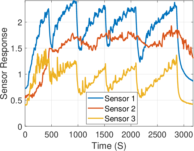

In the second case, we assume that we only have a single sensor. For example, the sensor 3 produces impulsive spikes between 0 and 1200 as shown in Fig.1a (in orange). Similar to the PCA-based denoising methods [12, 16] we form data vectors from neighboring temporal data windows and form the measurement data matrix where is the number of data windows and we have samples in each window. We form the kernel covariance matrix and compute its eigenvalues and eigenvectors . We reconstruct the data matrix using the first eigenvectors where is the eigenvector corresponding to the largest eigenvalue. After this step we compare the actual data vectors with the reconstructed ones . The vectors significantly different from the reconstructed vectors are considered to be anomalous. We let and observed that it is sufficient for anomaly detection.
Complexity Analysis: To calculate the covariance matrix , we perform multiplications and additions because we perform multiplications in each dot product. On the other hand, to calculate the -kernel covariance matrix , we perform sign operations, min operations and additions. According to Table I in [17], a multiplication operation consumes about 4 times more energy compared to the MF-operations in compute-in-memory (CIM) implementation at 1 GHz operating frequency. In this letter, we have three sensors and we used an Arduino to collect data so energy efficiency will not be significant but it will be significant in a large network with its own hardware. Since the value of or is much smaller than the vector length or , the eigenvector computation is negligible compared to the covariance matrix construction in this task. As a result, the -kernel PCA is about 4 times more energy efficient in CIM implementation. It is also more energy efficient in many other processors because multiplications consume more energy than additions and subtractions. [18].
Contribution: In our recent work [11] we introduced the -kernel PCA, while this paper introduces a novel method to employ the -kernel PCA into the anomaly detection problem. Our experiments show that in the anomaly detection task, the -kernel PCA produces better results than the regular PCA, the recursive -PCA [13] and the efficient -PCA via bit flipping [14] in our data set obtained from chemical sensors.
| Regular PCA | -PCA via Bit Flipping [14] | -Kernel PCA | |||||||
|---|---|---|---|---|---|---|---|---|---|
| Segment (Time/S) | Sensor 1 | Sensor 2 | Sensor 3 | Sensor 1 | Sensor 2 | Sensor 3 | Sensor 1 | Sensor 2 | Sensor 3 |
| 0–249 | 7.54 | 9.44 | 2.20 | 8.12 | 9.01 | 2.37 | 8.01 | 9.08 | 2.21 |
| 250–499 | 25.61 | 18.48 | 9.23 | 21.82 | 23.66 | 8.71 | 19.54 | 27.64 | 7.24 |
| 500–749 | 11.81 | 12.19 | 17.13 | 16.46 | 9.23 | 16.57 | 14.06 | 10.96 | 16.59 |
| 750–999 | 0.71 | 24.75 | 1.08 | 0.76 | 25.86 | 0.85 | 0.75 | 25.26 | 0.90 |
| 1000–1249 | 3.03 | 9.11 | 11.88 | 2.93 | 9.04 | 12.08 | 3.14 | 8.70 | 12.35 |
| 1250–1499 | 4.57 | 7.02 | 1.30 | 6.03 | 6.48 | 1.89 | 4.64 | 6.92 | 1.38 |
| 1500–1749 | 5.71 | 31.50 | 2.79 | 10.60 | 30.41 | 1.16 | 7.84 | 30.97 | 1.73 |
| 1750–1999 | 3.77 | 28.11 | 3.52 | 1.31 | 40.71 | 0.87 | 3.32 | 29.27 | 3.01 |
| 2000–2249 | 1.29 | 14.74 | 2.04 | 1.13 | 15.34 | 1.83 | 1.46 | 14.61 | 2.13 |
| 2250–2499 | 2.09 | 26.11 | 3.55 | 1.94 | 25.57 | 5.40 | 1.98 | 25.95 | 3.88 |
| 2500–2749 | 5.08 | 6.08 | 7.39 | 5.13 | 5.53 | 8.61 | 4.95 | 6.32 | 7.37 |
| 2750–2999 | 1.09 | 10.67 | 1.87 | 1.05 | 10.91 | 1.77 | 1.17 | 10.66 | 1.86 |
| 3000–3249 | 0.98 | 12.89 | 3.51 | 0.92 | 13.22 | 3.30 | 0.99 | 12.94 | 3.51 |
| Regular PCA | -PCA via Bit Flipping [14] | -Kernel PCA | |||||||
|---|---|---|---|---|---|---|---|---|---|
| Segment (Time/S) | Sensor 1 | Sensor 2 | Sensor 3 | Sensor 1 | Sensor 2 | Sensor 3 | Sensor 1 | Sensor 2 | Sensor 3 |
| 0–249 | 1.82 | 11.52 | 1.32 | 2.04 | 11.31 | 1.43 | 2.09 | 11.29 | 1.45 |
| 250–499 | 2.55 | 1.30 | 1.06 | 2.52 | 1.35 | 1.10 | 2.52 | 1.35 | 1.06 |
| 500–749 | 13.63 | 11.07 | 6.61 | 13.97 | 11.38 | 6.19 | 13.55 | 10.91 | 6.93 |
| 750–999 | 4.62 | 6.93 | 1.36 | 4.63 | 6.90 | 1.41 | 4.37 | 7.42 | 1.25 |
| 1000–1249 | 3.28 | 1.76 | 1.85 | 3.22 | 1.77 | 2.01 | 3.25 | 1.81 | 1.86 |
| 1250–1499 | 4.76 | 50.56 | 1.51 | 3.67 | 52.57 | 1.21 | 5.12 | 50.12 | 1.92 |
| 1500–1749 | 1.68 | 28.23 | 0.92 | 2.03 | 27.83 | 1.08 | 2.10 | 27.71 | 1.20 |
| 1750–1999 | 0.98 | 21.09 | 3.91 | 0.98 | 21.09 | 3.92 | 1.22 | 20.74 | 4.20 |
| 2000–2249 | 2.65 | 18.01 | 18.88 | 2.83 | 17.34 | 19.43 | 2.41 | 20.60 | 17.05 |
| 2250–2499 | 5.67 | 4.72 | 1.41 | 5.67 | 4.73 | 1.40 | 5.52 | 4.95 | 1.39 |
| 2500–2749 | 3.62 | 1.58 | 0.61 | 3.58 | 1.63 | 0.63 | 3.57 | 1.65 | 0.62 |
| 2750–2999 | 1.97 | 1.55 | 1.81 | 1.96 | 1.58 | 1.79 | 1.98 | 1.61 | 1.78 |
| 3000–3249 | 5.54 | 50.49 | 1.79 | 3.67 | 54.51 | 0.92 | 5.72 | 50.23 | 1.99 |
| 3250–3499 | 3.58 | 37.25 | 1.29 | 4.62 | 35.78 | 1.93 | 3.13 | 38.00 | 1.06 |
| 3500–3749 | 2.53 | 35.25 | 4.93 | 1.23 | 40.35 | 3.07 | 2.42 | 35.53 | 4.78 |
3 Experimental Results
We collected data using three ammonia MQ137 Tin oxide (SnO2) based sensors [19]. Sensors are connected to an Arduino Uno board, and the sampling rate is 2 samples per second. Sensors and a cylindrical ammonia source are placed in an airtight chamber. Sensors are pre-heated for 48 hours before collecting the data. When SnO2 is heated and exposed to the air, it reacts with the oxygen present in the air and form a layer of negative ion on the surface and reduce the surface conductivity [19]. When ammonia vapor comes in contact with the surface, it combines with the oxide ion layer on the top and releases electrons for conduction. As a result, the conductivity of the surface increases. This change in surface resistance can be measured in the form of voltage. Our experimental setup is shown in Fig. 2.

Multiple Sensor Anomaly Detection: The three sensors are placed close to each other and one of the sensors (sensor 2) is obstructed with a cylindrical cover with multiple holes. The cover causes the sensor to react more slowly than the other sensors to the ammonia build-up and release. The obstruction level of the outlier sensor is adjusted in each trial to avoid over-fitting to one condition. Moreover, to generate a more realistic environment with varying levels of ammonia concentration, the chamber lid is opened at random intervals and with random duration. Opening and closing the lid is repeated multiple times to create different rise and fall responses. Sensor waveforms from two experiments are shown in Fig. 1.
We apply the -kernel PCA based anomaly detection method described in Section 2.1 to the data obtained from the three sensors. We compared the proposed method with the regular -PCA, the recursive -PCA [13] and the efficient -PCA via bit flipping [14]. The later two compute . Tolerance parameter of the recursive -PCA method is set as as suggested by the authors [13]. We plot the Receiver Operating Characteristic (ROC) curve in Fig. 3 and compute the Area Under Curve (AUC) scores for each method. As shown in Table 3 states, the -kernel PCA provides the highest AUC score, and the recursive -PCA [13] provides the lowest AUC score in this case. This is probably due to the non-convex optimization method that they use to compute the principle vector, and the method requires a suitable tolerance parameter. On the other hand, the -kernel PCA does not need any tolerance parameters and the eigenvector computations are equivalent to the computational load of the regular PCA.

| Method | AUC score | AUC Increment |
|---|---|---|
| Regular PCA (baseline) | 0.7366 | - |
| Recursive -PCA [13] | 0.7203 | -0.0163 |
| -PCA via bit flipping [14] | 0.7203 | -0.0163 |
| -kernel PCA | 0.7483 | 0.0117 |
CSD values of the sensors’ response in Fig. 1a using different PCAs are listed in Table 1, and CSD values of the sensors’ response in Fig. 1b are listed in Table 2, respectively. The threshold values 21.63 for the regular PCA, 21.64 for the -PCA via bit flipping [14] and 21.61 for the -kernel PCA are computed from the normal cases obtained from other experiments. We have different threshold values for the regular PCA and the -kernel PCA because they have different principle eigenvectors. Even if we use the same threshold (21.60) the classification results in Tables 1 and 2 will not change.
Sensor 2 does not always exhibit anomalous behavior. In general, its response increases due to ammonia gas exposure but not decrease as fast as the other sensors when there is no gas as shown in Fig. 1. The regular PCA detects the anomalous behavior of Sensor 2 in 9 out of 28 data segments. On the other hand, the -PCA via bit flipping and our -kernel PCA detect the anomalous behavior of Sensor 2 in 10 out of 28 data segments. Moreover, the regular PCA and the -PCA via bit flipping produce a false alarm in the second data segment (250 - 499 seconds) of Sensor 1 as shown in Table 2, while our -kernel PCA avoids this false alarm case. In conclusion, -kernel PCA produces better results than the regular PCA, the recursive -PCA [13] and -PCA via bit flipping [14].
Anomaly Detection Using a Single Sensor: During the first three ammonia gas exposures, the sensor 3 positively responds but it also produces spikes up to 1200s as shown in Fig. 1a. Multisensor PCA-based anomaly detection cannot detect this behavior because only the sensor 1 works properly before 1200s. However, we compare the current sensor window of Sensor 2 with its neighboring data windows we can identify the anomalous behavior. We used data segments to construct the covariance and -kernel covariance matrices. In each data segment we have measurement. We used only the dominant eigenvector to estimate the data segments.
The regular PCA, the -PCA via bit flipping, and the -kernel PCA reconstructed waveforms do not have spikes and that is how we can identify the anomaly in sensor readings as shown in Fig. 4. Table 4 shows the CSD values of these methods and they correctly identified the anomolous segments.
| Segment | Regular PCA | -PCA via Bit Flipping | -Kernel PCA |
|---|---|---|---|
| 1 | 9.62 | 9.51 | 9.79 |
| 2 | 13.59 | 13.64 | 13.55 |
| 3 | 7.21 | 7.30 | 7.26 |
| 4 | 4.35 | 4.58 | 4.38 |
| 5 | 3.48 | 3.62 | 3.65 |


4 Conclusion
In this paper, we presented a framework for detecting anomalous sensors and sensor measurements in a chemical sensory system using the -kernel PCA. We collected data from three commercial Tin Oxide (SnO2) sensors by exposing them to ammonia in an environment-controlled experiment. The proposed -kernel PCA is more robust than the regular PCA in our experiments. This is due to the fact that -kernel PCA is related with the -norm and it gives less emphasis to anomalous spikes in sensor measurements while computing the correlation matrix. The computational energy cost of the -kernel PCA is much lower than the regular PCA on many processors. Because of low energy complexity, the -kernel PCA can be implemented in low-cost edge devices directly connected to the chemical sensors.
References
- [1] Alexander Vergara, Shankar Vembu, Tuba Ayhan, Margaret A Ryan, Margie L Homer, and Ramón Huerta. Chemical gas sensor drift compensation using classifier ensembles. Sensors and Actuators B: Chemical, 166:320–329, 2012.
- [2] Fatih Erden, E Birey Soyer, B Ugur Toreyin, and A Enis Cetin. Voc gas leak detection using pyro-electric infrared sensors. In 2010 IEEE International Conference on Acoustics, Speech and Signal Processing, pages 1682–1685. IEEE, 2010.
- [3] Diaa Badawi, Hongyi Pan, Sinan Cem Cetin, and A Enis Çetin. Computationally efficient spatio-temporal dynamic texture recognition for volatile organic compound (voc) leakage detection in industrial plants. IEEE Journal of Selected Topics in Signal Processing, 14(4):676–687, 2020.
- [4] U Mittal, Jitender Kumar, AT Nimal, MU Sharma, et al. Single chip readout electronics for saw based gas sensor systems. In 2017 IEEE SENSORS, pages 1–3. IEEE, 2017.
- [5] Hilmi E Egilmez and Antonio Ortega. Spectral anomaly detection using graph-based filtering for wireless sensor networks. In 2014 IEEE International Conf. on Acoustics, Speech and Signal Processing, pages 1085–1089. IEEE, 2014.
- [6] Ling Huang, XuanLong Nguyen, Minos Garofalakis, Michael I Jordan, Anthony Joseph, and Nina Taft. In-network pca and anomaly detection. In NIPS, volume 2006, pages 617–624, 2006.
- [7] Vassilis Chatzigiannakis and Symeon Papavassiliou. Diagnosing anomalies and identifying faulty nodes in sensor networks. IEEE Sensors Journal, 7(5):637–645, 2007.
- [8] Laura Erhan, M Ndubuaku, Mario Di Mauro, Wei Song, Min Chen, Giancarlo Fortino, Ovidiu Bagdasar, and Antonio Liotta. Smart anomaly detection in sensor systems: A multi-perspective review. Information Fusion, 67:64–79, 2021.
- [9] Yuan Yao, Abhishek Sharma, Leana Golubchik, and Ramesh Govindan. Online anomaly detection for sensor systems: A simple and efficient approach. Performance Evaluation, 67(11):1059–1075, 2010.
- [10] A Sree and K Venkata. Anomaly detection using principal component analysis. Journal of Computer Science and Technology, 5 (4), pages 124–126, 2014.
- [11] Hongyi Pan, Diaa Badawi, Erdem Koyuncu, and A. Enis Cetin. Robust principal component analysis using a novel kernel related with the -norm. In 2021 29th European Signal Processing Conference (EUSIPCO), pages 2189–2193, 2021.
- [12] B. Schölkopf, A. Smola, and K. Müller. Kernel principal component analysis. In Artificial Neural Networks — ICANN’97, Lecture Notes in Computer Science, vol 1327, Heidelberg, Berlin, Germany, 1997.
- [13] Panos P Markopoulos, George N Karystinos, and Dimitris A Pados. Optimal algorithms for -subspace signal processing. IEEE Transactions on Signal Processing, 62(19):5046–5058, 2014.
- [14] Panos P Markopoulos, Sandipan Kundu, Shubham Chamadia, and Dimitris A Pados. Efficient l1-norm principal-component analysis via bit flipping. IEEE Transactions on Signal Processing, 65(16):4252–4264, 2017.
- [15] Cem Emre Akbaş, Osman Günay, Kasım Taşdemir, and A Enis Çetin. Energy efficient cosine similarity measures according to a convex cost function. Signal, Image and Video Processing, 11(2):349–356, 2017.
- [16] SB Mike, B Scholkopf, and AJ Smola. Kernel pca and denoising in feature space. Advances in Neural Information Processing System, pages 524–536, 1999.
- [17] Shamma Nasrin, Ahish Shylendra, Yuti Kadakia, Nick Iliev, Wilfred Gomes, Theja Tulabandhula, and Amit Ranjan Trivedi. Enos: Energy-aware network operator search for hybrid digital and compute-in-memory dnn accelerators. arXiv preprint arXiv:2104.05217, 2021.
- [18] Shamma Nasrin, Diaa Badawi, Ahmet Enis Cetin, Wilfred Gomes, and Amit Ranjan Trivedi. Mf-net: Compute-in-memory sram for multibit precision inference using memory-immersed data conversion and multiplication-free operators. IEEE Trans. Circuits and Systems, 2021.
- [19] Joseph Watson, Kousuke Ihokura, and Gary SV Coles. The tin dioxide gas sensor. Measurement Science and Technology, 4(7):711, 1993.