Standard Young Tableaux and Lattice Paths

In this short paper, we use lattice path counting arguments to develop a generating function for the number of standard Young tableaux of shape $\lambda$, which we denote $f^{\lambda}$. From there, a well-known formula for $f^{\lambda}$ can be derived. The formula is not new, and neither do we claim to have discovered a new generating function. What is new (as far as can be determined) is the connection between lattice paths and $f^{\lambda}$. Moreover, the Fourier methods of Kicey and the author [1] provide an interesting (albeit not necessarily useful) formula for $f^{\lambda}$ where the height of $\lambda$ is no greater than 3.

We assume that the reader is familiar enough with the basic ideas of Young tableaux. No deep representation theory is required. The following definitions are fairly standard in the literature (e.g. [7, 8, 10]). Fix $r\in\mathbb{N}$. A partition $\lambda=(\lambda_{1},\lambda_{2},\ldots,\lambda_{r})$ will have the property that $\lambda_{i}\geq\lambda_{j}$ as long as $i\leq j$. For convenience, we allow $\lambda_{i}=0$. Necessarily, all zero parts will occur at the end of the sequence. If $\lambda_{r}>0$, then we say that $\lambda$ has height $r$. Denote the size of $\lambda$ by $|\lambda|=\lambda_{1}+\lambda_{2}+\cdots+\lambda_{r}$. The number of standard tableaux of shape $\lambda$ will be denoted by $f^{\lambda}$. Denote by $\Sigma_{r}$ the symmetric group on the $r$ letters, which acts on $r$-tuples $\mathbf{x}=(x_{1},x_{2},\ldots,x_{r})$ by permuting entries:

For any $r\in\mathbb{N}$, let $\mathbf{r}=(0,1,2,\ldots,r-1)$, and denote by $\mathbf{r}^{\ast}$ the reversed $r$-tuple, $(r-1,r-2,\ldots,1,0)$. Let $x_{1},x_{2},\ldots,x_{r}$ be formal commuting variables, and let $\mathbf{x}=(x_{1},x_{2},\ldots x_{r})$. Furthermore, if $\mathbf{m}=(m_{1},m_{2},\ldots,m_{r})$, then let $\mathbf{x}^{\mathbf{m}}=x_{1}^{m_{1}}x_{2}^{m_{2}}\cdots x_{r}^{m_{r}}$. Let $V_{r}$ be the Vandermonde polynomial,

Finally, let $t_{r}=\sum_{i=1}^{r}x_{i}$. We will be working with Laurent polynomials in the variables $\{x_{1},x_{2},\ldots x_{r}\}$. For such a function $f$, let $[f]_{\mathbf{m}}$ be the coefficient of the term $\mathbf{x}^{\mathbf{m}}$. The following theorem is already present (at least implicitly) in the literature. For example, Fulton and Harris develop the tools in §4 of [7].

Theorem 1 implies that $F_{n,r}=\frac{t_{r}^{n}V_{r}}{\mathbf{x}^{\mathbf{\mathbf{r}^{*}}}}$ is a generating function for the numbers $f^{\lambda}$ where $\lambda$ is a partition of $n$ having up to $r$ components. Theorem 1 directly implies the following formula, which is well-known in the literature [7].

where $\mu_{k}=\lambda_{k}+r-k$.

Fix $r\in\mathbb{N}$ and consider the set,

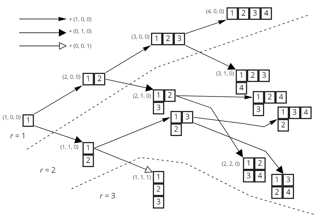
We may consider elements $\lambda\in\Lambda^{r}\subseteq\mathbb{N}_{0}^{r}$ to be partitions, points, or vectors as necessary. Each $\lambda\in\Lambda^{r}$ fits into a directed graph determined by the order in which the number labels are inserted into the Ferrers diagram of the Young tableau. For example, for $\lambda=(3,1)$ there are $f^{\lambda}=3$ ways to fill in the Young tableau, as suggested by Figure 1. (Note, the shape $(3,1)$ is equivalent to $(3,1,0)$). Each step in the directed graph adds 1 to one of the components of the vector, as long as the vector components remain non-increasing after the addition. Thus, if $\lambda=(1,1)$, then $\lambda+(1,0)=(2,1)$ is legal, but $\lambda+(0,1)=(1,2)$ is not.

Let

There is a recursive formula,

where $f^{\mu}=0$ whenever $\mu$ is not a legal partition – that is, whenever $\mu\notin\Lambda^{r}$. We take the convention that there is exactly one trivial Young tableau, corresponding to $\lambda=\mathbf{0}=(0,0,\ldots,0)$, so we have $f^{\mathbf{0}}=1$.

The key to our argument is to interpret partitions $\lambda$ as points in the lattice $\mathbb{N}_{0}^{r}$ with move set $\{\delta_{i}\;|\;1\leq i\leq r\}$, where a move in the direction $\delta_{i}$ is viewed as appending and labeling a new square to the tableau at row $i$. Thus each path that remains entirely within $\Lambda^{r}$ (the legal partitions) beginning at the origin and ending at the point $\lambda$ represents a distinct way to fill in the Ferrers digram of shape $\lambda$, and conversely every standard Young tableau has an associated lattice path within $\Lambda^{r}$ determined by its numberic labels. Therefore, the count of all such lattice paths from $\mathbf{0}$ to $\lambda$ is equal to $f^{\lambda}$. See Figure 2 for examples of the lattice $\Lambda^{r}$ for $r=2$ and $r=3$.

Counting paths in $\Lambda^{r}$ is complicated by the restrictions on legal partitions $\lambda$. A simple shift of the lattice by $\mathbf{r}^{*}$ suffices to make things easier. Indeed, this shift will also allow Eqn. (4) to be defined more explicitly in terms of identifying exactly when $\lambda-\delta_{i}$ is a legal partition. Let

Observe, if $\lambda\in\Lambda^{r}$ and $\lambda-\delta_{i}\notin\Lambda^{r}$, then it must necessarily be the case that $\lambda-\delta_{i}+\mathbf{r}*$ has either an entry equal to $-1$ or a repeated entry.

Inspired by methods found in Ault and Kicey [2, 1], consider functions $v:\widetilde{\Lambda}^{r}\to\mathbb{Z}$, which may be extended to $v:\mathbb{N}_{0}^{r}\to\mathbb{Z}$ in a manner to be explained presently.

For convenience, we assume all $\Sigma$-admissible functions $v$ take the value $v({\bf{x}})=0$ if any component of ${\bf{x}}$ is negative. Thus, if $v:\widehat{\Lambda}^{r}\to\mathbb{Z}$, then there is a unique, well-defined extension of $v$ to a function (also called $v$) such that $v:\mathbb{Z}^{r}\to\mathbb{Z}$ and $v$ is $\Sigma$-admissble; namely, set $v({\bf{x}})=0$ whenever ${\bf{x}}$ has negative or repeated entries and $v(\sigma{\bf{x}})=\mathrm{sgn}(\sigma)v({\bf{x}})$ whenever ${\bf{x}}\notin\widehat{\Lambda}^{r}$ has distinct non-negative entries.

For each $1\leq i\leq r$, let $R_{i}$ “right-shift” operator defined on functions $v:\mathbb{Z}^{r}\to\mathbb{Z}$ by

Let $T_{r}=\sum_{i=1}^{r}R_{i}$.

Define $v_{0}:\widetilde{\Lambda}^{r}\to\mathbb{Z}$ such that $v_{0}(\mathbf{r}^{*})=1$ and $v_{0}({\bf{x}})=0$ for ${\bf{x}}\neq\mathbf{r}^{*}$, and extend $v_{0}$ to a $\Sigma$-admissible function. For each $n\in\mathbb{N}$, let $v_{n}=T_{r}^{n}[v_{0}]$, which by Lemma 5 is $\Sigma$-admissible.

Finally, we make the connection to Eqn. (2). Recall $V_{r}$ from Eqn. (1). There are exactly $r!$ nonzero terms, including ${\bf{x}}^{\mathrm{r}^{*}}$, whose coefficient is 1. It should be clear from its form as a sum of terms of the form $\mathrm{sgn}(\sigma){\bf{x}}^{\sigma(\mathbf{r^{*}})}$ that $V_{r}$ is the (ordinary) generating function corresponding to $v_{0}$. Moreover, the transition operator $T_{r}$ corresponds to multiplication by $t_{r}=x_{1}+\cdots+x_{r}$. Thus, the generating function that counts the number of $n$-length paths in $\widetilde{\Lambda}^{r}$ from $\mathbf{r}^{*}$ to ${\bf{x}}$ is precisely $t_{r}^{n}V_{r}$. That is, $t_{r}^{n}V_{r}$ is the generating function for $v_{n}$. Lemma 7 then implies that a shift of exponents is needed to get the generating function for $f^{\lambda}$; namely, reduction of all multi-exponents by $\mathbf{r}^{*}$, which corresponds to division by ${\bf{x}}^{\mathbf{r}^{*}}$ in the generating function. This completes the argument and proves Theorem 1.

The functions $v_{n}({\bf{x}})$ defined above may be interpreted in a different way – as walks in Weyl alcoves. For $n\in\mathbb{N}_{0}$, let $\Lambda^{r}_{n}=\{\lambda\in\Lambda\;|\;|\lambda|=n\}$, which we call the $n$th slice of $\Lambda^{r}$. Observe that $\Lambda^{r}_{n}$ is a subset of the plane $x_{1}+x_{2}+\cdots+x_{r}=n$. This plane can be viewed as an affine lattice $A_{n-1}$, whose move set is determined by the simple roots $\alpha_{i}=\delta_{i}-\delta_{i+1}$. Then $\Lambda_{n}^{r}$, with an appropriate shift, exists within the interior points of an alcove in $A_{n-1}$.

We shall focus on the case $r=3$, that is, we shall develop a formula to count $f^{\lambda}$ where $\lambda=(a,b,c)$, as this is precisely the case for which methods of Ault-Kicey [1] will be useful and interesting. (Unfortunately, the Fourier methods of Ault-Kicey do not easily scale beyond $A_{2}$ lattices. For more about walks in arbitrary Weyl alcoves and related structures, see [4, 5, 6, 9].) Let $A_{2}$ be defined in the usual way as a lattice in the plane generated by roots $\alpha=(1,0)$ and $\beta=(-1/2,\sqrt{3}/2)$, as shown in Figure 3. Thus, all points of $A_{2}$ take the form $\langle u,v\rangle=u\alpha+v\beta$ for $u,v\in\mathbb{Z}$.

Consider the affine transformation,

With $u=x-z+2$ and $v=y-z+1$ as defined by Eqn. (6), we have $u>v$ and $v>0$. This implies that $P(x,y,z)$ lies in the interior of the region bounded by the $\alpha$-axis and $\alpha+\beta$-axis. We also find that since $x\leq n$, then $u=x-z+2\leq n+2$. That is, $P(\Lambda_{n}^{3})$ lies entirely within the triangular region determined by $u>v$, $v>0$, and $u<n+3$ in $A_{2}$.

Moreover, the three moves, $\delta_{1}=(1,0,0)$, $\delta_{2}=(0,1,0)$, and $\delta_{3}=(0,0,1)$, in $\Lambda^{3}$ transform to the following moves in $A_{2}$:

Thus, counting paths in $\Lambda^{3}$ is equivalent to counting paths in a triangular lattice of sufficiently large size, say $a+1$ points along a side (where $\lambda=(a,b,c)$ is the shape for which we wish to count $f^{(a,b,c)}$, where $a+b+c=n$) with move set $\{\alpha,\beta,-\alpha-\beta\}$. Refering to the notation and methods established in Appendix B of [1], the relevant transition operator is $T^{+}=R^{\alpha}+R^{\beta}+R^{-\alpha-\beta}$, and so we have on the Fourier side,

The Fourier-transformed initial state is defined by

Now, according to Theorem B.1 of [1], $v_{n}=\mathcal{F}^{-1}\left[\widehat{T^{+}}^{n}V_{0}\right]$ is the vertex function that counts the paths in the wedge that we are interested in. Here $\mathcal{F}$ is a discrete Fourier transform, and $\mathcal{F}^{-1}$ is its inverse. Adjusting the input by the affine transformation Eqn. (6), we have produced an interesting formula for height-3 standard Young tableaux.

The author concedes that Eqn. (8) may be of very little practical use to those who actually wish to count $f^{\lambda}$, except perhaps as a curiosity. However, the formula is fairly easy to code into a computer algebra system such as Sage [11], and has been verified to produce correct counts of $f^{\lambda}$.

The investigation into partitions and Young tableaux was inpired by a recent talk by Robert (Bob) Donley [3]. Bob¹¹ 1 Bob Donley teaches as the Queensborough Community College (New York, NY) and is an organizer of the Representation Theory Seminar at the CUNY Graduate Center. provided many insightful suggestions that helped to shape the direction of this paper. I am also grateful to Cyril Banderier and the other organizers of the virtual conference, “Lattice Paths, Combinatorics and Interactions,” hosted by the Centre International de Rencontres Mathématiques (June 2021) for accepting my poster presentation, “From Lattice Paths to Standard Young Tableaux.”

References

• [1] S. Ault and C. Kicey. Counting Lattice Paths Using Fourier Methods. Applied and Numerical Harmonic Analysis. Springer International Publishing, 2019.
• [2] S. V. Ault and C. Kicey. Counting paths in corridors using circular Pascal arrays. Discrete Mathematics, 332(6):45–54, October 2014.
• [3] Robert Donley. “Vandermonde convolution for ranked posets.” New York Number Theory Seminar: Combinatorial and Additive Number Theory (CANT 2021).
• [4] I. M. Gessel and C. Krattenthaler. Cyclic partitions. Transactions of the American Mathematical Society, 349:429–479, 1997.
• [5] I. M. Gessel and D. Zeilberger. Random walk in a Weyl chamber. Proceedings of the American Mathematical Society, 115:27–31, 1992.
• [6] D. Grabiner. Random walk in an alcove of an affine Weyl group, and non-colliding random walks on an interval. Journal of Combinatorial Theory, Series A, 97(2):285–306, Feb. 2002.
• [7] W.F.J. Harris, W. Fulton, and J. Harris. Representation Theory: A First Course. Graduate Texts in Mathematics. Springer New York, 1991.
• [8] I.G. Macdonald. Symmetric Functions and Hall Polynomials. Oxford classic texts in the physical sciences. Clarendon Press, 1998.
• [9] Paul R. G. Mortimer and T. Prellberg. On the number of walks in a triangular domain. Preprint.
• [10] R. P. Stanley. Algebraic Combinatorics: Walks, Trees, Tableaux, and More. Springer-Verlag, New York, 2013.
• [11] W. Stein. Sagemath. http://www.sagemath.org. last accessed April, 2017.