A three-dimensional (3D) topological insulator has gapless surface states with a conical dispersion [1, 2]. This Dirac cone is protected by Kramers degeneracy, no perturbation that preserves time-reversal symmetry can gap it out — provided that the top and bottom surfaces remain uncoupled, to prevent Dirac cones from annihilating pairwise [3].

To study the dynamics of Dirac fermions on a computer, one needs to discretize the Dirac equation

for the two-component spinor $\Psi(\bm{r},t)$ (with velocity $v$ and Pauli spin matrices $\sigma_{\alpha}$). The electrostatic potential $V$ preserves time-reversal symmetry, so one would expect the Dirac cone to remain gapless for any time-reversally invariant discretization scheme that avoids fermion doubling [4] (only zero-energy states at momentum $\bm{k}=0$).

The objective of our paper is, firstly, to demonstrate that this expectation is incorrect, it does not apply to the split-operator technique [5] for the discretization of the time-evolution operator, which is commonly used [6, 7, 8] because of its computational efficiency. Then, secondly, we will show how a “drop-in” modification of the algorithm can restore a gapless Dirac cone — without reducing the computational efficiency (scaling as $N\ln N$ in the number of lattice sites).

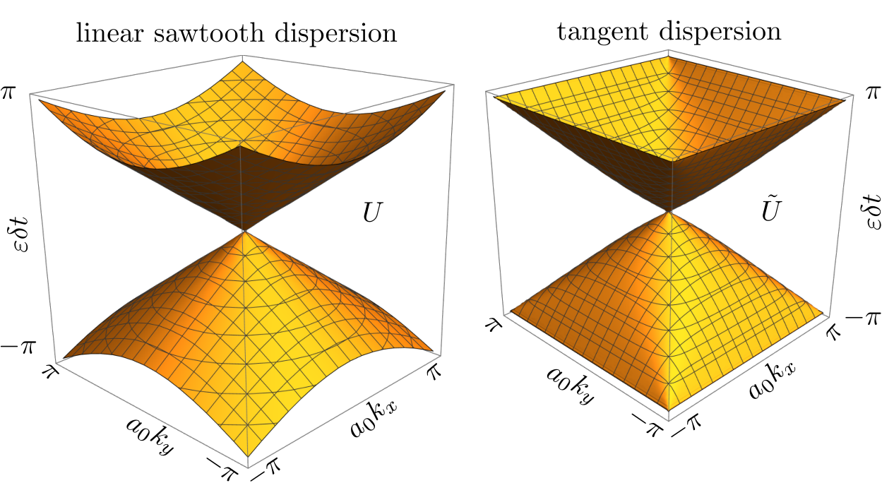
We consider a 2+1-dimensional space-time lattice with lattice constants $a_{0}$ in space and $\delta t$ in time. In the split-operator technique the derivative operator $d/dx$ is evaluated in momentum representation as the linear function $k$ in the first Brillouin zone $|k|<\pi/a_{0}$ — periodically repeated as a sawtooth for larger momenta. The drop-in modification that we propose is to replace $k$ by $(2/a_{0})\tan(a_{0}k/2)$. The computational efficiency of the algorithm is not compromised, but the effect on the quasi-energy–momentum band structure is crucially important: While the linear sawtooth dispersion introduces discontinuous derivatives at Brillouin zone boundaries, the tangent dispersion produces a smooth band structure, see Fig. 1. As we will show, a potential that varies rapidly on the scale of $a_{0}$ is able to gap out the Dirac cone in the former case but not in the latter case.

By way of introduction, before we embark on the space-time discretization, we first discuss the simpler time-independent problem, when only space is discretized.

Consider a one-dimensional (1D) lattice along the $x$-axis, and first take $V\equiv 0$. Different ways to discretize the derivative $d/dx$ will produce different energy-momentum dispersion relations $\pm E(k)$. (The $\pm$ sign distinguishes the chirality of the massless Dirac fermions, left-movers versus right-movers.) What all dispersions have in common is that they are periodic with period $2\pi/a_{0}$ and vanish linearly at $k=0$. We compare three alternatives, see Fig. 2.

The local discretization $df/dx\mapsto[f(x+a_{0})-f(x-a_{0})]/(2a_{0})$ gives a sine dispersion

which vanishes also at the boundary $|k|=\pi/a_{0}$ of the first Brillouin zone (fermion doubling). A nonlocal discretization, which couples $f(x)$ to distant lattice points, can remove the spurious Dirac cone at nonzero momentum. The socalled “slac discretization” [9, 10] produces a dispersion relation that is strictly linear within the first Brillouin zone $|k|<\pi/a_{0}$. The dispersion has the $2\pi$-periodic sawtooth form¹¹ 1 The function $\text{mod}\,(q,2\pi,-\pi)\equiv q-2\pi\left\lfloor\frac{q+\pi}{2\pi}\right\rfloor\in[-\pi,\pi)$ gives $q$ modulo $2\pi$ with an offset $-\pi$. (The floor function $\lfloor x\rfloor$ returns the greatest integer $\leq x$.) The mod function is discontinuous at $q=\pi$, jumping from $-\pi$ to $\pi$, we arbitrarily assign to $\text{mod}\,(\pi,2\pi,-\pi)$ the value of $-\pi$. The choice $\text{mod}\,(\pi,2\pi,-\pi)\equiv 0$ would produce in Fig. 3 an isolated doubly degenerate state at $E=0=k$, disconnected from the slac bands.

Now apply the staggered potential $V(x)=V\cos(\pi x/a_{0})$, switching from $+V$ to $-V$ between even and odd-numbered lattice sites. This potential couples the states at $k$ and $k+\pi/a_{0}$, as described by the Hamiltonian

The Brillouin zone is halved to $|k|<\pi/2a_{0}$, with the band structure

A gap opens in the Dirac cone for both the local and slac discretizations, of size

What we learn from this simple calculation is that removing the second cone at $|k|=\pi/a_{0}$ is not enough to protect the Dirac cone at $k=0$ from becoming gapped if the potential varies rapidly on the scale of the lattice constant. What happens is that the large gap $\Delta$ in the dispersion at $k=\pi/a_{0}$ is folded onto $k=0$ by the staggered potential, resulting in a minigap $\delta E=V^{2}/\Delta$ for $V\ll\Delta$. To avoid the gap opening we thus need a pole $\Delta\rightarrow\infty$ in the dispersion at the Brillouin zone boundary.

An alternative discretization due to Stacey [11] gives the dispersion

with a pole at $k=\pi/a_{0}$. And indeed, substitution of Eq. (1.7) into Eq. (1.5) shows that no gap opens at $k=0$ (see Fig. 3).

The merits of the Stacey discretization for the time-independent problem were studied in Refs. [12] (at the level of the scattering matrix) and in Ref. [13] (at the level of the Hamiltonian). It was shown that the eigenvalue equation $H\Psi=E\Psi$ can be discretized into a generalized eigenvalue problem ${\cal H}\Psi=E{\cal P}\Psi$ with local Hermitian tight-binding operators on both sides of the equation.²² 2 The Stacey discretization is local in the sense that the operators ${\cal H}$ and ${\cal P}$ in the generalized eigenvalue problem ${\cal H}\Psi=E{\cal P}\Psi$ can be represented by sparse Hermitian matrices. If we would write this as a strict (non-generalized) eigenvalue problem, ${\cal P}^{-1}{\cal H}\Psi=E\Psi$, we would find that the operator ${\cal P}^{-1}{\cal H}$ is nonlocal (it is not sparse). There is therefore no violation of the Nielsen-Ninomiya no-go theorem [4], which only applies to strict eigenvalue problems. Basically, a local formulation of the generalized eigenvalue problem is possible because tangent is the ratio of sine and cosine, which represent local tight-binding operators on a lattice. If all one would care about would be the presence of a pole in the dispersion at $k=\pi/a_{0}$, one could work with other functions than the tangent, but the tangent dispersion combines this property with the possibility of a local algorithm.

So much for the introduction to the time-independent discretization. In what follows we turn to the dynamical problem, by generalizing the approach of Refs. [11, 12, 13] to the discretization of space and time. In the next section 2 we show that the time discretization removes the pole in the tangent dispersion, which becomes a smooth function of momentum $\bm{k}$ and quasi-energy $\varepsilon$ (yellow bands in Fig. 1). In Sec. 3 we then prove that the Dirac point remains gapless for any perturbation that preserves either time-reversal symmetry or chiral symmetry — even if it varies rapidly on the scale of the lattice constant.

In contrast, the quasi-energy bandstructure of the linear sawtooth dispersion has discontinuous derivatives at the Brillouin zone boundaries (red bands in Fig. 1). These spoil the protection of the Dirac cone, which is gapped by a staggered potential.

A key feature of the approach presented in Sec. 2 is that it requires only a small modification of the usual split-operator technique, involving the replacement of the linear momentum operator appearing in the time-evolution operator by its tangent. Since this operator is evaluated in momentum representation, the replacement is immediate. It does not degrade the computational efficiency of the algorithm, which retains the favorable $N\ln N$ scaling in the number of lattice sites (limited only by the efficiency of the fast Fourier transform).

An alternative implementation which is fully in real space is possible, taking the form of an implicit finite-difference equation $A\Psi(t+\delta)=B\Psi(t)$ with sparse matrices $A$ and $B$. This formulation is a bit more cumbersome to explain, we present it an appendix.

The Dirac Hamiltonian

is the sum of a kinetic term that depends on momentum $\bm{k}$ and a potential term that depends on position $\bm{r}$. (We set $\hbar$ to unity.) The split-operator technique [5] separates these two terms in the time-evolution operator,

with an error term that is of third order in the time slice $\delta t$ [14].

Space is discretized on a square or cubic lattice (lattice constant $a_{0}$ in each direction). The periodicity of the Brillouin zone is enforced by the substitution

In 1D this is the linear sawtooth dispersion of Fig. 2, red curve. A discrete fast Fourier transform is inserted between the kinetic and potential terms, so that each is evaluated in the basis where the operators $\bm{k}$ and $\bm{r}$ are diagonal. The computational cost scales as $N\ln N$ for $N$ lattice sites.

The eigenvalues $e^{i\varepsilon\delta t}$ of the unitary operator $U$ define the quasi-energies $\varepsilon$ modulo $2\pi/\delta t$. For free motion, $V=0$, these are given by

The 2+1 dimensional band structure in the first Brillouin zone

is plotted in Fig. 4 for $v=a_{0}/\delta t$, when the dispersion is strictly linear along the $k_{x}$ and $k_{y}$-axes. (Alternatively, for $v=2^{-1/2}\,a_{0}/\delta t$ the dispersion is strictly linear along the diagonal lines $k_{x}=\pm k_{y}$, the corresponding plots are in App. A.)

The band structure repeats periodically upon translation by $\pm 2\pi/a_{0}$ in the $k_{x},k_{y}$ directions and by $\pm 2\pi/\delta t$ in the $\varepsilon$ direction. Upon crossing a zone boundary the dispersion has a discontinuous derivative, see Fig. 5.

To remove the discontinuity at the Brillouin zone boundary we modify the kinetic term in the evolution operator (2.2) in two ways: Firstly we approximate the exponent by a rational function (Cayley transform [15, 16]),

The error of third order in the time slice is of the same order as the error in the operator splitting, Eq. (2.2).

Secondly we replace $k_{\alpha}$ by $(2/a_{0})\tan(a_{0}k_{\alpha}/2)$, defining the modified evolution operator

We abbreviated $\chi(k)=(v\delta t/a_{0})\tan(a_{0}k/2)$ and $\sigma_{0}$ is the $2\times 2$ unit matrix. This looks more complicated than Eq. (2.2), but it can be computed equally efficiently since in both equations each operator is evaluated in the basis where it is diagonal.

The required periodicity when $k_{\alpha}\mapsto k_{\alpha}+2\pi/a_{0}$ is automatically ensured by the replacement of the linear momentum by the tangent, it does not need to be enforced by hand as in Eq. (2.3). Although $\tan(a_{0}k_{\alpha}/2)$ has a pole when $k_{\alpha}=\pi/a_{0}$, this pole is removed in the evolution operator (2.7) — which has no singularity at the Brillouin zone boundaries.

The eigenvalues $e^{i\varepsilon\delta t}$ of $\tilde{U}$ for free motion, $V=0$, are given by

plotted in Figs. 6 and 7. Comparison with Figs. 4 and 5 shows that the zone boundaries are now joined smoothly. The dispersion is approximately linear near $\bm{k}=0$ and exactly linear along the lines $k_{x}=0$ and $k_{y}=0$ if we choose the discretization units such that $v=a_{0}/\delta t$. (See App. A for the case $v=2^{-1/2}\,a_{0}/\delta t$, when the linear dispersion is along $k_{x}=\pm k_{y}$.)

The condition of time-reversal symmetry for the unitary evolution operator $U$ reads

where the complex conjugation should be taken in the real space representation, when $\bm{k}=-i\nabla$ changes sign. The time-reversal operator, $\sigma_{y}\times\text{complex conjugation}$, squares to $-1$, so Kramers theorem applies: In the presence of a periodic potential $V$, when momentum $\bm{k}$ remains a good quantum number, the eigenvalues at $\bm{k}=0$ should be at least doubly degenerate.³³ 3 Kramers theorem may be more familiar for a Hermitian operator, the proof for a unitary operator proceeds similarly: If $U\psi=e^{i\phi}\psi$ with $\phi\in\mathbb{R}$, and $\sigma_{y}U^{\ast}\sigma_{y}=U^{-1}$, then $U\sigma_{y}\psi^{\ast}=\sigma_{y}(\sigma_{y}U^{\ast}\sigma_{y}\psi)^{\ast}=\sigma_{y}(U^{-1}\psi)^{\ast}=e^{i\phi}\sigma_{y}\psi^{\ast}$, thus $\psi$ and $\sigma_{y}\psi^{\ast}$ are eigenstates of $U$ with the same eigenvalue. They cannot be linearly related, because if $\psi=\lambda\sigma_{y}\psi^{\ast}$ for some $\lambda\in\mathbb{C}$, then $\sigma_{y}\psi^{\ast}=-\lambda^{\ast}\psi=-|\lambda|^{2}\sigma_{y}\psi^{\ast}$, which is impossible for $\psi\neq 0$. Hence the eigenvalue $e^{i\phi}$ is at least doubly degenerate.

Kramers degeneracy implies a band crossing at $\bm{k}=0$ — provided that the bands depend smoothly on $\bm{k}$ — hence this applies to the evolution operator $\tilde{U}$ for the tangent dispersion, but not to the operator ${U}$ for the linear sawtooth dispersion. We conclude that the Dirac point of $\tilde{U}$ is protected by time-reversal symmetry, while the Dirac point of $U$ is not.

We demonstrate this difference for the checkerboard potential

(The calculation is described in App. B.) In Fig. 8 we show the three ways in which this potential can affect the Dirac point. The evolution operator $\tilde{U}$ shows the modification $T_{0}$, while $U$ shows $T_{-}$, see Fig. 9. The other option $T_{+}$ appears in Fig. 3 and in App. A.

Chiral symmetry of the evolution operator is expressed by

Since $U^{-1}=U^{\dagger}$, this implies that $U$ can be decomposed in the block form

We consider a 2D periodic potential, so that momentum $\bm{k}=(k_{x},k_{y})$ is a good quantum number. The band structure has winding number [17]

along a contour $\Gamma$ in the Brillouin zone on which $\det B$ does not vanish.⁴⁴ 4 One has $\det B\neq 0$ on $\Gamma$ if the quasi-energy $\varepsilon(\bm{k})$ does not cross 0 or $\pi$ on that contour [17]. This prevents us from extending the contour along the entire first Brillouin zone, when the winding number should vanish. This is a topological invariant, it cannot change in response to a continuous perturbation [18]. A Dirac point within the contour is signaled by $W=\pm 1$. While pairs of Dirac points of opposite winding number can annihilate, a single Dirac point is protected by chiral symmetry — provided that the evolution operator is continuous.

The 2D Dirac Hamiltonian has chiral symmetry when $V\equiv 0$. An in-plane magnetization

preserves the chiral symmetry. We are thus led to compare the two evolution operators

Both satisfy the chiral symmetry relation (3.3), $\tilde{U}$ is a continous function of $\bm{k}$ while $U$ is not.

The implication for the stability of the Dirac point is shown in Fig. 10, where we compare the bandstructure in the presence of the checkerboard magnetization

(see App. B). A gap opens for $U$ (linear sawtooth dispersion), while the Dirac point for $\tilde{U}$ (tangent dispersion) remains unaffected.

References

- [1] M. Z. Hasan and C. L. Kane, Topological insulators, Rev. Mod. Phys. 82, 3045 (2010) doi:10.1103/RevModPhys.82.3045.
- [2] X.-L. Qi and S.-C. Zhang, Topological insulators and superconductors, Rev. Mod. Phys. 83, 1057 (2011) doi:10.1103/RevModPhys.83.1057.
- [3] C. L. Kane, Topological band theory and the invariant, Contemporary Concepts of Condensed Matter Science 6, 3 (2013) doi:10.1016/B978-0-444-63314-9.00001-9.
- [4] H. B. Nielsen and M. Ninomiya, A no-go theorem for regularizing chiral fermions, Phys. Lett. B 105, 219 (1981) doi:10.1016%2F0370-2693%2881%2991026-1.
- [5] J. W. Braun, Q. Su, and R. Grobe, Numerical approach to solve the time-dependent Dirac equation, Phys. Rev. A 59, 604 (1999) doi:10.1103/PhysRevA.59.604.
- [6] P. Krekora, Q. Su, and R. Grobe, Klein paradox in spatial and temporal resolution, Phys. Rev. Lett. 92, 040406 (2004) doi:10.1103/PhysRevLett.92.040406.
- [7] G. R. Mocken and C. H. Keitel, FFT-split-operator code for solving the Dirac equation in 2+1 dimensions, Comput. Phys. Commun. 178, 868 (2008) doi:10.1016/j.cpc.2008.01.042.
- [8] F. Fillion-Gourdeau, E. Lorin, and A. D. Bandrauk, Numerical solution of the time-dependent Dirac equation in coordinate space without fermion-doubling, Comput. Phys. Commun. 183, 1403 (2012) doi:10.1016/j.cpc.2012.02.012.
- [9] S. D. Drell, M. Weinstein, and S. Yankielowicz, Strong-coupling field theories. II. Fermions and gauge fields on a lattice, Phys. Rev. D 14, 1627 (1976) doi:10.1103/PhysRevD.14.1627.
- [10] J. P. Costella, A new proposal for the fermion doubling problem, arXiv:hep-lat/0207008. https://arxiv.org/abs/hep-lat/0207008
- [11] R. Stacey, Eliminating lattice fermion doubling, Phys. Rev. D 26, 468 (1982) doi:10.1103/PhysRevD.26.468.
- [12] J. Tworzydło, C. W. Groth, and C. W. J. Beenakker, Finite difference method for transport properties of massless Dirac fermions, Phys. Rev. B 78, 235438 (2008) doi:10.1103/PhysRevB.78.235438.
- [13] M. J. Pacholski, G. Lemut, J. Tworzydło, and C. W. J. Beenakker, Generalized eigenproblem without fermion doubling for Dirac fermions on a lattice, SciPost Phys. 11, 105 (2021) doi:10.21468/SciPostPhys.11.6.105.
- [14] M. Suzuki, Fractal decomposition of exponential operators with applications to many-body theories and Monte Carlo simulations, Phys. Lett. A 146, 319 (1990) doi:10.1016/0375-9601(90)90962-N.
- [15] N. Watanabe and M. Tsukada, Fast and stable method for simulating quantum electron dynamics, Phys. Rev. E 62, 2914 (2000) doi:10.1103/PhysRevE.62.2914.
- [16] A. Chaves, L. Covaci, Kh. Yu. Rakhimov, G. A. Farias, and F. M. Peeters, Wave-packet dynamics and valley filter in strained graphene, Phys. Rev. B 82, 205430 (2010) doi:10.1103/PhysRevB.82.205430.
- [17] K. Mochizuki, T. Bessho, M. Sato, and H. Obuse, Topological quantum walk with discrete time-glide symmetry, Phys. Rev. B 102, 035418 (2020) doi:10.1103/PhysRevB.102.035418.
- [18] S. Ryu, A. P. Schnyder, A. Furusaki, and A. W. W. Ludwig, Topological insulators and superconductors: Tenfold way and dimensional hierarchy, New J. Phys. 12, 065010 (2010) doi:10.1088/1367-2630/12/6/065010.
- [19] C. Roiesnel, Definition of the covariant lattice Dirac operator, Phys. Rev. D 87, 074505 (2013) doi:10.1103/PhysRevD.87.074505.
- [20] A. Donís Vela, G. Lemut, M. J. Pacholski, J. Tworzydło, and C. W. J. Beenakker, Reflectionless Klein tunneling of Dirac fermions: Comparison of split-operator and staggered-lattice discretization of the Dirac equation, J. Phys. Cond. Matt. 34, 364003 (2022) doi:10.1088/1361-648X/ac7d2d.
- [21] A. George, Nested dissection of a regular finite element mesh, SIAM J. Numer. Anal. 10, 345 (1983) doi:10.1137/0710032.
- [22] A. George and E. Ng, On the complexity of sparse QR and LU factorization of finite-element matrices, SIAM J. Sci. Stat. Comput. 9, 849 (1988) doi:10.1137/0909057.
- [23] X. S. Li and J. W. Demmel, SuperLU_DIST: A scalable distributed-memory sparse direct solver for unsymmetric linear systems, ACM Trans. Math. Softw. 29, 110 (2003) doi:10.1145/779359.779361.
- [24] The computer code used in Sec. C.2 to test the efficiency of the split-operator and finite-difference algorithms will be made available at the Zenodo repository: https://dx.doi.org/10.5281/zenodo.7057254