Spectral and Energy Efficient User Pairing for RIS-assisted Uplink NOMA Systems with Imperfect Phase Compensation
Abstract
Non-orthogonal multiple access (NOMA) is considered a key technology for improving the spectral efficiency of fifth-generation (5G) and beyond 5G cellular networks. NOMA is beneficial when the channel vectors of the users are in the same direction, which is not always possible in conventional wireless systems. With the help of a reconfigurable intelligent surface (RIS), the base station can control the directions of the channel vectors of the users. Thus, by combining both technologies, the RIS-assisted NOMA systems are expected to achieve greater improvements in the network throughput. However, ideal phase control at the RIS is unrealizable in practice because of the imperfections in the channel estimations and the hardware limitations. This imperfection in phase control can have a significant impact on the system performance. Motivated by this, in this paper, we consider an RIS-assisted uplink NOMA system in the presence of imperfect phase compensation. We formulate the criterion for pairing the users that achieves minimum required data rates. We propose adaptive user pairing algorithms that maximize spectral or energy efficiency. We then derive various bounds on power allocation factors for the paired users. Through extensive simulation results, we show that the proposed algorithms significantly outperform the state-of-the-art algorithms in terms of spectral and energy efficiency.
Index Terms:
Energy efficiency, non-orthogonal multiple access, power allocation, reconfigurable intelligent surface, spectral efficiency, uplink, user pairing.I Introduction
In the fifth-generation (5G)and beyond 5Gcommunication systems, significant improvements are expected in terms of spectral efficiency, energy conservation, massive connectivity, and latency requirements. Non-orthogonal multiple access (NOMA)is considered as a key multiple access technique to enhance the spectral efficiency of future cellular networks [1]. Various NOMAtransmission schemes have been evaluated for possible consideration of NOMAin 5Guplink scenario [2]. In NOMA, multiple users are allocated with the same time and frequency resources to achieve multi-fold improvement in the network throughputs. However, the users are multiplexed in either power domain (power-domain NOMA) or code domain (code-domain NOMA), which requires the receiver to employ a successive interference cancellation (SIC)and decode the data [3]. Similar to NOMA, RISis considered as a key technology to improve the spectral efficiency of the cellular networks [4]. An RISis a two-dimensional planar array consisting of low-cost reflecting antenna elements that can modify the amplitude and phase of the signal. Thus, by using RIS, the BScan perform beamforming and transmit the signal in the desired direction.
Unlike the spatial multiplexing in orthogonal multiple access (OMA), NOMA is beneficial in situations where the channel vectors of users are in the same direction [4]. This is not always possible in conventional wireless systems, whereas, in the case of RIS-assisted systems, the BScan control the direction of the user channel vectors by tuning the RIS [4, 5]. For these reasons, RIS-assisted NOMAsystems have been widely considered to achieve significant improvements in the network performance [4, 6]. However, the ideal phase control is difficult to achieve in practice for various reasons like hardware impairments, channel estimation errors, etc. These imperfections in the phase control degrade the achievable spectral and energy efficiencies in the network. Further, in NOMAsystems, the achievable data rates are significantly dependent on the user pairing, and hence, while pairing the users in RIS-assisted NOMAsystems, the network operator has to consider the imperfections in the phase compensation. Otherwise, the expected improvements in the network throughputs will not be realized in practice. For the aforementioned reasons, investigating the effect of imperfection in phase at the RISis crucial to achieve optimum system performance.
In [7, 8], the authors have proposed various channel estimation techniques for RIS-assisted wireless systems. In [9, 10], the authors have formulated the sum-rate maximization as an optimization problem, and then, derived a near-optimal solution for RIS-assisted uplink NOMAsystems. However, limited works in the literature have considered the imperfection in phase for the downlink OMAand NOMAsystems [6, 11, 12]. To the best of our knowledge, none of the existing works considered the imperfections in the phase compensation while pairing the users in RIS-assisted uplink NOMAsystems. Motivated by this, we present the following key contributions in this paper.
- •
For RIS-assisted uplink NOMAsystems, we derive bounds on imperfection in the phase compensation to achieve minimum required data rates.
- •
We propose user pairing algorithms that maximize spectral efficiency and energy efficiency, respectively.
- •
We derive bounds and define the power allocation factors for the paired users.
- •
Through extensive simulation results, we show that the proposed algorithms significantly outperform the state-of-the-art algorithms.
The rest of the paper is organized as follows. The system model is presented in Section II. In Section III, we propose the adaptive user pairing algorithms, derive the bounds on the power allocation factors, and formulate the criterion for pairing the users to maximize spectral and energy efficiencies. In Section IV, we present the simulation results for various scenarios. Section V presents some concluding remarks and possible future works.
II System Model
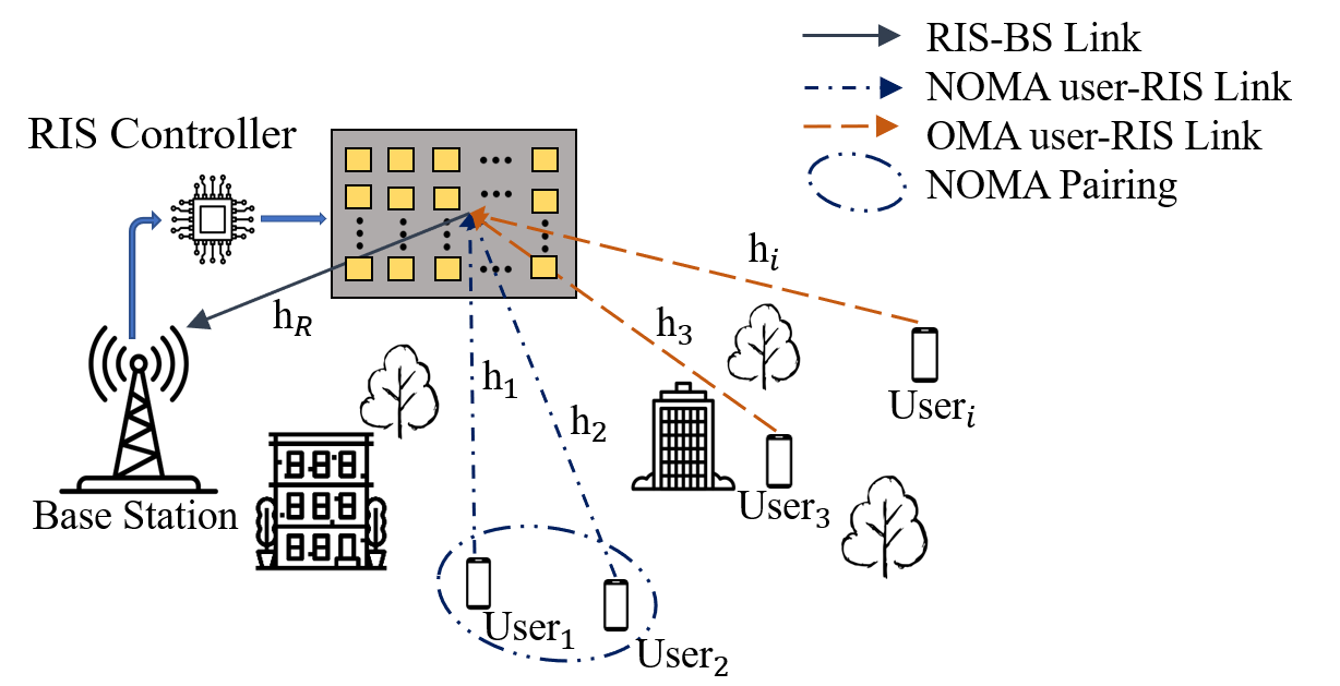
We consider an uplink scenario with antennae at the BS, reflective antenna elements at the RIS, and a single antenna at each user as shown in Fig. 1. The direct link between the BSand user is assumed to be blocked by the obstacles such as buildings, trees, or human body which is a likely scenario in case of mmwave communications [11]. Further, the channel coefficients from user to RISand RISto BSare defined as and , respectively and are formulated as follows [11]
| (1) | ||||
| (2) |
where and denote the channel gains from user to RISand RISto BS, respectively, and represent the angle of departure (AoD)in azimuth and elevation at the RIS, respectively, and represent angle of arrival (AoA)in azimuth and elevation at the BS, respectively, and represent the AoAin azimuth and elevation at the RIS, respectively, and represents the array response vector. A uniform square planar array (USPA)with antenna elements, has elements in both horizontal and vertical directions, and thus, the array response vector is defined as
where, is the equispaced elemental distance, is the signal wavelength, are the indices of the USPAelements in the horizontal and vertical directions, respectively.
We denote the reflection matrix at the RISas and define it as follows [4].
where, is the phase shift introduced by reflecting element at the RIS. However, note that the ideal phase control is difficult to achieve in practice because of various reasons like hardware limitations, imperfect channel state information, etc. For this reason, we consider imperfections in the phase control and define the practical reflection matrix as follows.
where, with being the error in phase control at antenna element. Further, we assume to be uniformly distributed over , . Thus, in the case of OMAtransmission, the signal received from the user at the BSis formulated as
where denotes the Hermitian of a matrix, is the available transmit power at each user, is the data symbol transmitted by the user, and denotes the thermal noise. The signal to interference plus noise ratio (SINR)of an user in an RIS-assisted OMAsystem is formulated as
| (3) |
where is the interference power and is the noise variance. In the case of RISassisted NOMA, we consider two users multiplexed in power domain, with channel coefficients and . Additionally, we assume the following
Thus, the BSreceives (+), where and are the data symbols transmitted by the strong and weak user, respectively. Further, we consider a fractional power control scenario, where represent the fraction of the total available transmit power used by the strong and weak users, respectively. Thus, the signal received from the user in an RIS-assisted NOMAsystem is formulated as follows
| (4) |
From (4), we define the SINRof the users in RIS-assisted NOMAas follows
| (5) | ||||
| (6) |
From (1)-(2), we define the following [6]:
| (7) |
We adopt the following approximation from [11]:
| (8) |
where follows the strong law of large numbers [11], in , the expectation of odd function vanishes over the interval , and is obtained by using the probability density function , where . Substituting (8) in (7)
Using these approximations, we define the channel state information (CSI)of user as
| (9) |
Using (9) in (3), (5), and (6), we formulate the received SINRs as follows
Given a logarithmic rate model, the normalized achievable data rates by the users in OMAand NOMAare formulated as [12]
| (10) | ||||
| (11) | ||||
| (12) |
Next, we propose various adaptive user pairing algorithms.
III Proposed Algorithms
In this section, we propose MPAand EEPAalgorithms to maximize the sum rate and energy efficiency, respectively. Additionally, in both the algorithms, we derive a criterion for pairing the users in NOMAwhich ensures the minimum required data rates are achieved for each user. We denote and as the minimum required data rates by the strong and weak users, respectively. Thus, both MPAand EEPAalgorithms should satisfy the following constraints
| (13) | |||
| (14) |
III-A MPA
In MPA, apart from satisfying (13)-(14), we allocate the transmit powers (and ) that maximize the ASRof the paired users, where, ASRis defined as
We formulate the desired optimization as follows.
| (15) | ||||
| s.t. | ||||
| (16) | ||||
| (17) |
III-A1 Bounds on and
| (18) |
Thus, ASRis an increasing function with respect to and . However, from (11), an increase in will decrease the achievable data rate for the strong user, whereas, there is no such impact with an increase in . Hence, to maximize the ASR, we assign . Thus, we get,
| (19) |
| (20) |
| (21) |

III-A2 Criterion for pairing the users
Using (20)-(21), and assuming , we obtain the pairing criterion for the MPAalgorithm as follows.
| (22) |
We define and as the achievable OMArates, and then, pair the users in NOMAiff (22) is satisfied. Otherwise, we consider transmitting the information for the users in an OMAscenario as shown in Fig. 2. This way, the proposed algorithm ensures that a minimum of OMArates are achieved in a worst-case scenario and it maximizes the ASRby switching to NOMAwhenever feasible.
III-A3 Power allocation
For the paired users, we define the power allocation factors as follows.
| (23) | ||||
| (24) |
Note that in (23), the strong user transmits at maximum power to maximize the spectral efficiency, whereas, in (24), the weak user transmits at a maximum possible power that does not degrade the strong user’s data rate beyond the OMArate. Further, to avoid transmit power violations, we limit the maximum value of to 1 in (24).
Lemma 1.
Proof.
For the ease of understanding, we define
| (25) | ||||
| (26) |
Thus, we reformulate (15) as follows
| (27) | ||||
| s.t. | (28) | |||
| (29) | ||||
| (30) |
where, (27) is obtained by using the fact that logarithmic function is a monotonically increasing function and substituting (18) in (15). The constraint (28) is obtained by substituting (25)-(26) in (13) and the constraint (29) is obtained by further solving the (14). Additionally, since , are non negative, we get , and thus, we consider the constraint (16) is already captured in (28)-(29). Next, the Lagrangian for (27) is formulated as
Solving stationarity conditions , we get
| (31) | ||||
| (32) |
The complementary slackness conditions are formulated as
| (33) | ||||
| (34) | ||||
| (35) | ||||
| (36) |
The dual feasibility conditions are formulated as
| (37) |
Solving (31)-(37), we find that the possible optimal values of are and . From (27), larger the values of and , larger will be the ASR. Since, has no impact on any of the desired constraints, we consider only the solutions with which are , and . Note that considering will violate the constraint (28). Hence, by substituting , the optimal values of (,) are either or . Since, , we conclude as the optimal solution. This completes the proof of the Lemma 1. ∎
Next, we present the EEPAalgorithm.


III-B EEPA
In EEPA, apart from satisfying (13)-(14), we allocate the powers (and ) that maximize the energy efficiency (EE)of the paired users, where, EEis defined as
Thus, we formulate the optimisation problem as follows.
| (38) | ||||
| s.t. |
III-B1 Criterion for pairing the users
Solving (28) for a worst case scenario of , we get,
| (39) |
Thus, we define the upper bound on the phase imperfection in EEPAas
| (40) |
We define and as the achievable OMArates, and then, pair the users in NOMAiff the imperfection in the phase compensation is less than . Otherwise, we consider transmitting the information for the users in an OMAscenario as shown in Fig. 2.
III-B2 Power allocation
IV Numerical Results


For the simulations, we have considered , , and . We have then dropped the BSs and users from Poisson point distribution with densities of 25 BS/km2 and 2000 users/km2, respectively. For each user, we have calculated the path loss and the received signal power from each BSby considering the urban cellular path loss model presented in [15]. The users are then associated to the BSfrom which they receive the maximum signal power, and the rest of the BSs are considered as interfering BSs. Given this simulation set-up, we have calculated various performance metrics with the proposed and the existing state-of-the-art algorithms which are summarised as follows.
In Fig. 3, we present the achievable data rates for varying . For the evaluation, we consider two configurations of user pairs with , , and two configurations of imperfection in phase compensation, . As shown in Fig. 3, with increasing , the data rates for weak user increases. This increase in also increases interference for the strong user, and thus, the achievable data rate for the strong user decreases. Note that for a fixed , the achievable data rates and sum rate are better in Fig. 3(a) as compared to Fig. 3(c) because of the better SINRconditions. Further, with an increase in the , the achievable data rates and sum rate are smaller in Fig. 3(b) when compared to Fig. 3(a). As shown in Fig. 3, the ASRis a non-decreasing function of which aligns with our formulation in the Section III-A. Further, beyond the proposed , the individual data rates are not better than the OMAcounterparts. Thus, we validate the proposed bounds on power allocation factors in the presence of imperfect phase compensation.
In Fig. 4, we present the comparison of the achievable data rates for varying . For the evaluation, we consider two configurations of user pairs with dB and dB in Fig. 4(a) and Fig. 4(b), respectively. Further, we consider and while calculating the achievable data rates. With an increase in , the achievable rates decrease. Additionally, whenever , the achievable data rates and sum-rates are always better than the OMAcounterparts. Thus, we validate the proposed bound on the imperfection in the phase compensation. Note that a similar analysis is extendable for the EEPAscenario.


In Fig. 5, we present the performance comparison of mean of achievable data rates with various algorithms. As shown in Fig. 5, for both strong and weak user, the performance of sum rate maximisation (SRM) [9] declines gradually with increase in and the data rates fall below OMAfor larger . In case of the proposed algorithms, both MPAand EEPAconsider the imperfections in the phase compensation, and hence, the data rates gradually converge to OMAthe rates with an increase in . Further, as shown in Fig. 5(b), the SRMalgorithm tries to maximize the ASRand in the process significantly decreases the weak user data rates beyond the required OMArates. However, the MPAalgorithm maximizes the strong user rate to achieve maximum ASRand yet ensures both strong and weak user achieve minimum of OMArates. The EEPAalgorithm allocates minimum power to each user to ensure the minimum required OMArates are achieved, and hence, the data rates with EEPAare significantly lower than MPArates and slightly higher than the OMArates.

In Fig. 6, we present the comparison of the mean ASRwith the proposed algorithms against the SRMand OMAin the presence of imperfect phase compensation. As shown in Fig. 6, SRMachieves highest ASRas compared to all the algorithms. However, as shown in Fig. 5, the SRMdoes not achieve minimum required rates for the weak user, whereas, the proposed MPAmaximizes ASRwhile ensuring a minimum of OMArates for both strong and weak users. Further, note that with EEPA, the achievable sum rate is slightly higher than the OMArates.
In Fig. 7, we present the comparison of the mean achievable sum rate and energy efficiency with various algorithms. As shown in Fig. 7(a) and 7(b), the SRMhas highest mean ASRand EEat the lower . However, note that SRMalgorithm does not ensure that individual users achieve a minimum of OMArates. Further, with increasing , the mean ASRand EEof the both the proposed algorithms converge to the OMArates, whereas, the performance of the SRMdegrades significantly as compared to the OMArates. Hence, it is not always beneficial to pair the users in NOMA. Thus, we conclude that, the proposed algorithms outperform the existing algorithms in presence of imperfection in phase compensation. Additionally, they also maximize the data rates or energy efficiency while ensuring minimum required data rates for each user.


V Conclusion
We have proposed adaptive user pairing algorithms for RIS-assisted uplink NOMAsystems that maximize the achievable sum-rate or energy efficiency. We have formulated the criterion for user pairing based on the derived bounds on imperfection in the phase compensation. Through numerical results, we have validated the derived bounds and the proposed pairing criterion. Further, we have proposed novel power allocation procedures for the paired users. We have performed extensive system-level simulations and have shown that the proposed algorithms achieve significant improvement over the state-of-the-art algorithms with increase in phase imperfection. In the future, we plan to validate the proposed algorithms on the hardware test-beds.
References
- [1] A. Kassir et al., “Power Domain Non Orthogonal Multiple Access: A Review,” in Proc. TAFGEN, 2018, pp. 66–71.
- [2] 3GPP, “Study on Non-Orthogonal Multiple Access (NOMA) for NR,” Technical Report 38.812, v 16.0.0, Dec. 2018.
- [3] M. S. Ali et al., “Dynamic User Clustering and Power Allocation for Uplink and Downlink Non-Orthogonal Multiple Access (NOMA) Systems,” IEEE Access, vol. 4, pp. 6325–6343, 2016.
- [4] Z. Ding and H. V Poor, “A Simple Design of IRS-NOMA Transmission,” IEEE Commun. Lett., vol. 24, no. 5, pp. 1119–1123, 2020.
- [5] J.-C. Chen, “Machine Learning-Inspired Algorithmic Framework for Intelligent Reflecting Surface-Assisted Wireless Systems,” IEEE Trans. on Veh. Technol., pp. 1–1, 2021.
- [6] Pavan Reddy M. and A. Kumar, “User Pairing and Power Allocation for IRS-Assisted NOMA Systems with Imperfect Phase Compensation,” arXiv, cs.IT 2106.07938, 2021.
- [7] S. Xia and Y. Shi, “Intelligent Reflecting Surface for Massive Device Connectivity: Joint Activity Detection and Channel Estimation,” in Proc. IEEE ICASSP, 2020, pp. 5175–5179.
- [8] Z. Wang et al., “Channel Estimation for IRS-Assisted Multiuser Communications,” in Proc. IEEE WCNC, 2020, pp. 1–6.
- [9] M. Zeng et al., “Sum Rate Maximization for IRS-Assisted Uplink NOMA,” IEEE Commun. Lett., vol. 25, no. 1, p. 234–238, Jan 2021.
- [10] G. Yang et al., “Intelligent Reflecting Surface Assisted Non-Orthogonal Multiple Access,” in Proc. IEEE WCNC, 2020, pp. 1–6.
- [11] S. Zhou et al., “Spectral and Energy Efficiency of IRS-Assisted MISO Communication With Hardware Impairments,” IEEE Wireless Commun. Lett., vol. 9, no. 9, pp. 1366–1369, 2020.
- [12] N. S. Mouni et al., “Adaptive User Pairing for NOMA Systems With Imperfect SIC,” IEEE Wireless Commun. Lett., vol. 10, no. 7, pp. 1547–1551, 2021.
- [13] A. Zappone et al., “Energy Efficiency in Secure Multi-Antenna Systems,” arXiv, cs.IT 1505.02385, 2015.
- [14] M. Zeng et al., “Energy-Efficient Power Allocation for Uplink NOMA,” in Proc. IEEE GLOBECOM, 2018, pp. 1–6.
- [15] 3GPP, “Study on channel model for frequencies from 0.5 to 100 GHz,,” Technical Report 38.901, v 16.0.0, Jan. 2020.