Aerial Scene Parsing: From Tile-level Scene Classification to Pixel-wise Semantic Labeling*
Abstract
Given an aerial image, aerial scene parsing (ASP) targets to interpret the semantic structure of the image content, e.g., by assigning a semantic label to every pixel of the image. With the popularization of data-driven methods, the past decades have witnessed promising progress on ASP by approaching the problem with the schemes of tile-level scene classification or segmentation-based image analysis, when using high-resolution aerial images. However, the former scheme often produces results with tile-wise boundaries, while the latter one needs to handle the complex modeling process from pixels to semantics, which often requires large-scale and well-annotated image samples with pixel-wise semantic labels. In this paper, we address these issues in aerial scene parsing, with perspectives from tile-level scene classification to pixel-wise semantic labeling. Specifically, we first revisit aerial image interpretation by a literature review. We then present a large-scale scene classification dataset that contains one million aerial images termed Million-AID. With the presented dataset, we also report benchmarking experiments using classical convolutional neural networks (CNNs). Finally, we perform ASP by unifying the tile-level scene classification and object-based image analysis to achieve pixel-wise semantic labeling. Intensive experiments show that Million-AID is a challenging yet useful dataset, which can serve as a benchmark for evaluating newly developed algorithms. When transferring knowledge from Million-AID, fine-tuning CNN models pretrained on Million-AID perform consistently better than those pretrained ImageNet for aerial scene classification, demonstrating the strong generalization ability of the proposed dataset. Moreover, our designed hierarchical multi-task learning method achieves the state-of-the-art pixel-wise classification on the challenging GID, which is a profitable attempt to bridge the tile-level scene classification toward pixel-wise semantic labeling for aerial image interpretation. We hope that our work could serve as a baseline for aerial scene classification and inspire a rethinking of the scene parsing of high-resolution aerial images.
Index Terms:
Aerial image interpretation, Million-AID, scene classification, semantic segmentation, transfer learningI Introduction
Aerial image understanding is a task of primary importance for a wide range of applications such as precision agriculture [1], urban planning [2], and environmental monitoring [3]. An essential way toward understanding an aerial image is to perform a full-scene semantic structure interpretation, also denoted as aerial scene parsing (ASP), which aims to label each pixel in the image with a semantic category to which it belongs. With more and more aerial images being available, ASP has been a momentous but active topic in the field of remote sensing [4, 5, 6, 7]. Besides, pixel-wise semantics acquired by ASP is usually demanded as the imperative prerequisite in practical applications like land use/land cover investigation [8, 9, 10]. However, aerial images taken from the bird’s view with large imaging angles are always characterized with large scale, which implies that conventional computational method with pixel-wise analysis is hard to fulfill a full aerial scene parsing. Moreover, the highly complex content and image structure further increase the difficulty of identifying the semantics of pixels in an aerial image.

Faced with this situation, aerial scene parsing has been simplified as tile-level scene classification which integrates the complicated image features and content as a whole for semantic classification [11, 12, 13, 14, 15, 16, 17, 18, 19, 20]. However, the tile-level scene classification focuses on summarizing the thematic content within a local area while accurate semantics of individual pixels cannot be identified. To remedy this defect, the scene image can be divided into different regions for semantic identification. A feasible way is to split the scene image into regular grids, on which the patch-based classification can be performed for aerial scene parsing [21, 22, 23, 24]. Nevertheless, it usually produces coarse maps with blurred object edges. Moreover, object-based image analysis (OBIA) that extracts homogeneous entities by over-segmentation has been widely employed to achieve pixel-wise semantic labeling [25, 26, 27, 28, 29]. Even with great success, aerial scene parsing relies on OBIA suffers from parameter optimization [30, 31], feature selection [32], and modeling the complex relationship among different objects when reasoning their semantic meaning [4]. Recently, semantic segmentation based on fully convolutional networks (FCNs) [33, 34, 35, 36] provides an end-to-end aerial scene parsing framework that has been intensively approached [37, 38, 39, 5, 6, 7, 40]. Still, the optimization of FCN methods requires a large amount of pixel-wise annotation which is extremely labor-intensive and time-consuming to produce. Figure 1(a)(d) illustrate the conventional methods for aerial scene parsing by human annotation, tile-level classification, object-based analysis, and end-to-end semantic segmentation, respectively. From an overall perspective, the above methods for aerial scene parsing are typically performed in a separate way, of which advantages cannot be integrated. To change this situation, a great deal of effort must be paid by addressing the following critical issues:
- •
The divergence of aerial scene parsing prototypes in tile-level and pixel-wise classification. Pixel-wise classification has been intensively approached to produce fine-grained labeling result [41, 42, 43] while tile-level classification can only provides coarse semantic description of regions [11, 14, 17, 16, 19]. Currently, the continuous improvement of image resolution has brought us aerial images of large scale and rich detail. As a result, aerial scene parsing by pixel-wise classification becomes a challenging task because of the variant attributes of pixels and the high computational cost. From the perspective of image expression, the improvement of image resolution also greatly enhances the semantic homogeneity of pixels in local regions. Thus, the semantics of individual pixels in an aerial image is closely related to their contextual information rather than relying solely on their own. In this context, it is reasonable to consider the pixel as a unit centered by tile-level scene and bridge its gap to pixel-wise semantic labeling.
- •
The scarcity on exploring the transferability of semantic scene knowledge of aerial images. Currently, the lack of large-scale benchmark datasets has become a bottleneck that hampers the development of data-driven methods for aerial image interpretation, particularly the deep learning-based ones. To alleviate this situation, the conventional way is to employ CNN models pretrained on natural image archives (e.g., ImageNet [44]) as feature extractors or to fine-tune them on target aerial images. However, there are great differences between natural and aerial images in spectral properties, image structure, and spatial arrangement. Moreover, the semantic categories that define the scene content also vary significantly between natural and aerial images. Thus, the learned features obtained through the above methods can be biased in characterizing aerial image content. With this in mind, it is of great significance to explore the transferability of data-driven models adapted with pure aerial scene images and free up their potential for aerial image interpretation.
With these points in mind, this paper addresses aerial scene parsing that unifies tile-level scene classification and object-based image analysis to achieve pixel-wise semantic labeling as illustrated in Figure 1(e). For doing so, we first provide a review to depict aerial image interpretation. Then, we present a large-scale aerial scene classification dataset, i.e., Million-AID, on which the benchmarking experiments are performed to investigate how well the current CNNs perform for aerial scene classification. Finally, we conduct aerial scene parsing from tile-level scene classification to pixel-wise semantic labeling, where knowledge transferring from Million-AID is performed to improve the accuracy. To sum up, our main contributions are as follows:
- •
We provide a comprehensive literature review on aerial image interpretation by revisiting its development outline, ranging from pixel-wise image classification, segmentation-based image analysis, and tile-level image classification that are connected to the improvement of spatial resolution of aerial images.
- •
We released a new large-scale dataset, i.e., Million-AID, for aerial scene recognition and benchmark a number of classical CNN models on multi-class and multi-label aerial scene classification. To the best of our knowledge, Million-AID is one of the largest benchmark datasets in the remote sensing community. The experimental results also demonstrate that Million-AID is challenging but useful, and can serve as a large-scale benchmark for developing aerial scene classification algorithms.
- •
We conducted extensive experiments to verify the tremendous potential of transferring scene knowledge from tile-level annotated Million-AID to pixel-wise semantic labeling for aerial scene parsing. Experiments show that fine-tuning CNN models pretrained on Million-AID perform consistently better than those pretrained on ImageNet for aerial scene classification. Our proposed hierarchical multi-task learning method exploiting Million-AID and GID achieves the state-of-the-art on pixel-wise aerial image classification.
The remainder of this paper is organized as follows. Section II presents the review of aerial image interpretation. Section III introduces the proposed large-scale scene classification dataset, i.e., Million-AID. Section IV presents the comprehensive benchmarking experiments on Million-AID, including multi-class and multi-label aerial scene classification. Section V presents experiments tile-level scene classification and pixel-wise semantic labeling with knowledge transfer from Million-AID. Finally, in Section VI, we draw conclusions regarding this work.
II Revisiting Aerial Image Interpretation

With the progress of sensor technology, the spatial resolution of aerial images has experienced a continuous improvement [45, 46]. Figure 2 presents the milestones of earth observation satellites at different times. Accordingly, the improvement of aerial image resolution has greatly promoted the development of aerial image interpretation. In this section, we focus on a review by revisiting the interpretation tasks of aerial images and the outline is presented in Figure 2.
II-A Pixel-wise aerial image classification
In the early 1970s, aerial images are characterized with a low spatial resolution (e.g., LandSat-1 and MODIS images) where each pixel describes an area of thousands of square meters of the Earth’s surface. And the sizes of ground features or objects are usually smaller than the ground sampling distance of image pixels. Thus, each pixel is able to present a scene of a specific semantic category. Individual pixels are obviously distinct from each other owing to the difference in covered ground features. In this situation, semantic interpretation of aerial images mainly focuses on pixel-wise classification using spectral signatures [47, 48] and coarse textural features [49, 50, 51, 52]. To this end, sampling analysis is naturally employed [53, 54, 55] to construct desirable classification schemes. Typically, training samples that are representative to reflect the distribution and variation of the diverse semantic content of interest are selected to extract category information. Thus, classification methods based on statistical analysis are widely employed by estimating the probability of a pixel belonging to each of the possible classes [56, 42, 57, 58, 59, 60].
In order to obtain reliable classification results, a number of classifiers were also developed for the pixel-wise aerial image parsing, such as maximum likelihood methods [61, 62, 63], minimum distance to means algorithms [64, 65], K-nearest neighbors classifiers [66, 67], and tree-based techniques [68, 69]. However, statistical classification methods usually show insufficient ability in discriminating pixel units due to the variation of spectral and spatial characteristics influenced by imaging conditions and ground feature attributes. Faced with this situation, more sophisticated classifiers such as random forest [70, 71, 72, 73], sparse representation [74, 75, 76, 77, 63, 78], artificial neural network [79, 80], and kernel-based methods [75, 81, 78, 73] represented by support vector machine [82, 83, 84] were intensively explored by actively embracing the machine learning techniques. These methods have made dramatic progress in pixel-wise aerial image classification owing to their strong ability to discriminate the complex spectral and spatial characteristics of ground features.
Pixel-wise classification approaches assume that each pixel only belongs to a single semantic category and different categories are mutually exclusive. However, such an assumption can be inconsistent with reality due to the limitation of spatial resolution of aerial images [41, 85]. Specifically, more than one object or ground feature belonging to different semantic categories can be contained within a pixel as their scales are smaller than the spatial resolution of aerial images. As a result, the existence of mixed pixels comes to be a nonnegligible problem in the medium and coarse spatial resolution aerial images. This could lead to an appreciable interpretation result when employing the pixel-wise classification strategy. To overcome this problem, sub-pixel classification is considered as an alternative for more accurate aerial image interpretation [86, 87, 88, 89].
A number of approaches have been derived to address the sub-pixel aerial image classification, including soft or fuzzy theory [90, 91, 92], neural networks [93, 94, 95], regression modeling and analysis [96, 97, 98], and spectral mixture analysis [99, 100, 101, 102]. Among these methods, the fuzzy technique and spectral mixture analysis are most commonly employed to overcome the mixed pixel problem. Particularly, fuzzy representation is developed to estimate multiple and partial memberships of all candidate categories within a pixel, where the corresponding areal proportion of each category can be acquired. The spectral mixture analysis assumes the value of a pixel is a linearly or non-linearly combination of a set of specific endmember spectra [100, 101]. Thus, the selection of endmembers becomes the key point for designing an effective classifier [103, 104, 105, 106]. Even with a great improvement of classification accuracy, sub-pixel class composition estimated by fuzzy classification and spectral mixture analysis cannot provide the spatial distribution of land cover classes within pixels. To address this issue, the sub-pixel mapping approaches are developed [107, 108, 88, 95]. In this scheme, each pixel is divided into sub-pixels which are predicted to get single semantic labels. Limited by the spatial resolution, aerial images interpreted by pixel-wise classification still face challenges in acquiring satisfactory results due to the mixture and complexity of image content within single pixels.
II-B Segmentation-based aerial image analysis
With the development of sensor technology, the spatial resolution of aerial images is gradually improved to be much smaller than the scales of ground features. Thus, the detail of spectrum, texture, and geometric structure in the image becomes prominent. Under the circumstances, single pixels are no longer isolated units since the ground features and objects could be composed of a certain number of pixels knitted into an image full of spatial patterns [109]. And the improved image quality also significantly increases the within-class variability, which decreases the potential accuracy of pixel-based approach to classification [27]. As a result, the traditional interpretation system established with pixel-wise statistics and analysis for low-resolution aerial images, to some extent, is beginning to show cracks in classifying aerial images for required accuracy and generalization ability [26].
Faced with this situation, researchers turn their attention to the new paradigm of object-based image analysis (OBIA) or geographic-object-based image analysis (GEOBIA) [25, 109, 26, 27, 32, 28, 110], where geographical or image objects are considered as the basic units instead of individual pixels for image classification. The objects are considered to be homogeneous entities, located within an image and perceptually generated from pixel-groups, where each pixel-group is composed of similar digital values and possesses an intrinsic size, shape, and geographic relationship with the real-world scene component it models [111]. In general, the OBIA generates objects by image segmentation and then performs image classification on objects. Thus, image segmentation serves as the initial and critical part to produce the fundamental elements of OBIA [29, 110].
In high-resolution remote sensing images, ground objects are presented with much richer spectral, textural, structural, and contextual detail that reveals the pattern characteristics [27]. It enables the objects of interest to be extracted by spectrally-based and spatially-based segmentation approaches, among which mathematical morphology analysis plays a significant role [112, 28]. Hence, the thresholding [113, 114, 115] and feature space clustering [116] methods are typically employed to generate objects by spectral analysis based on the fact that homogeneous objects share similar spectral characteristics. For spatially-based segmentation, edge detection [117, 114, 118, 119] and region generation (e.g, region growing [113, 120], merging, and splitting [114, 121, 122]) techniques are conducted according to the discontinuity and similarity of object areas, respectively. However, edge-based methods are precise in boundary detection while facing problems in generating closed segments. By contrast, region-based methods have the advantage in generating closed regions while resulting in imprecise segment boundaries. As compensation, hybrid segmentation [123, 114, 124] that consider both the boundary and spatial information between adjacent regions show significant advantages in object segmentation.
However, objects acquired by segmentation can only provide homogeneous regions while lacking a semantic description. Thus, the object features are then extracted and embedded into a classifier to determine the semantic categories. In doing so, both the feature extraction and classifier design play crucial roles in classification performance [125, 126]. Owing to the overwhelming advantages in visual feature extraction and classification, CNN frameworks have recently been integrated into OBIA and triggered the new trend of object-based CNN (OCNN) for aerial image interpretation [127, 128, 29]. With the availability of high-resolution aerial images, object-based approaches become dominant in the task of aerial image interpretation over the past two decades. Even with a significant performance advantage compared with pixel-wise classification methods, the object-based classification methods face challenges in parameter setting and optimization (e.g., segmentation scale) [30, 31], which affect the segmentation quality as well as the final classification accuracy. In addition, the segmentation and classification of objects fall into a complicated and multi-step implementation pipeline, which inevitably limits the efficiency and increases the difficulty of model deployment.
To overcome the above deficiencies, the solution that simultaneously produces the segmented homogeneous areas and corresponding semantic categories becomes an imperious demand. In recent years, aerial image classification have been greatly facilitated by deep convolutional neural networks (DCNNs) [129, 38, 39, 130], among which the fully convolutional network (FCN) [33] and the improved architectures [34, 35, 36] provide an end-to-end segmentation and classification pipeline. In contrast with conventional methods, the advantage of DCNN lies in its capacity to extract shallow visual and deep semantic features by the elaborately designed hierarchical framework [37]. However, the down-sampled features in deep layers will lead to the resolution degradation for the final classification results, in which the uncertainty of boundaries and detail of different classes is a serious issue. To deal with these issues, the multi-scale features [131, 132, 133, 134] and contextual information [135, 128] are typically considered to enhance the feature representation ability. The atrous and paralleled dilation convolution [36] is utilized to preserve feature resolution [136]. With the improvement of network architectures, the classification accuracy of aerial images has witnessed a continuous improvement.
Apart from the evolution of networks, significant efforts have been paid to improve the performance of classification models. Typically, the spatial and spectral attributes of aerial images have been intensively addressed in pixel-wise classification [137, 138, 139]. Particularly, the integration of spatial and spectral information is commonly employed to address the challenge of large spatial variability of spectral signatures [140, 141, 142, 143]. Regarding the limitation of training samples and generalization ability, transfer learning has been intensively explored to address the limitation of training samples for CNN frameworks and reported promising classification results [8, 144, 145, 146]. The readers may go to one of the review papers for a more comprehensive perspective of semantic segmentation using deep learning techniques [37, 137, 138, 147, 143, 148, 149]. However, owing to the lack of large-scale datasets, many interpretation algorithms are locally-oriented, typically manifested in the validation of one or several images within local areas which would affect the generalization ability. And the CNN-based methods also suffer from computational burden when classifying aerial images of large size and huge volume due to the improvement of spectral and spatial resolution.
II-C Tile-level aerial image classification
Even with the impressive success achieved by object-based analysis, individual objects carry information independent to their neighbors and thus neglect the thematic meaning in their contextual environment, which could lead to inaccurate classification results. To alleviate this problem, the hierarchical and contextual model is developed by organizing individual objects into hierarchical groups for aerial image parsing [4]. However, the implementation of object detection and hierarchical contextual representation is complicated. Thus, the classification of the tile-level scene, which is able to incorporate visual features, content components, and spatial arrangements as a whole, becomes an effective way for aerial image interpretation. In the last decade, a handful of visual descriptors have been employed for aerial scene classification [11, 150, 15, 151, 17, 16, 19]. We refer interested readers to [11, 17, 16] for a survey of the low-level and middle-level visual features employed for aerial scene classification.
Owing to the increasing accessibility of aerial images, the data-driven approaches particularly CNN-based ones have shown a great advantage over the handcrafted-feature-based approaches for aerial scene classification. In the beginning, pretrained CNNs are usually employed as feature extractors owing to their simplicity and efficiency [13, 152, 153]. However, the representation of aerial scenes is a challenging task owing to the complexity of scene components and scale variation. To improve the feature discrimination ability, multi-scale images or features are extracted and fused to generate robust global representation for scene classification [152, 154, 153, 155, 156]. In fact, the semantic category of an aerial scene usually depends on the spatial arrangement and class-specific objects in the image. Thus, deep local structures related to scene category are addressed to improve the classification performance [157, 158, 159]. Recently, CNNs based on attention mechanism have been addressed to highlight more local semantics and discard the noncritical information [160, 161, 162, 156]. In general, learning powerful features for content representation is of great importance for aerial scene recognition.
With the improvement of spatial resolution of aerial images, the within-class diversity and between-class similarity of semantic scenes have been greatly increased, which makes scene recognition a challenging task. To relieve this issue, deep metric learning algorithms are developed to learn discriminative category features [163, 164, 165]. Particularly, the complex relationship pervading aerial scenes is further explored in the embedding space by learning deep graph networks [166, 167, 168]. The main idea is to map the scene features closely to each other for the same categories while as farther apart as possible for different categories. As conventional CNNs with a fixed architecture may show limitations in grasping the scene content of large diversity, automatically learning CNN architecture specified for aerial scenes has been intensively explored [169, 170, 171] and achieved encouraging results.
However, the methods based on deep learning require large-scale annotated samples for model adaption while most of them are trained and tested on relatively small-scale datasets. To overcome this problem, scene classification based on few-shot learning has recently attracted extensive attention [172, 173, 174]. Moreover, annotated scene images from different domains are also employed to relieve the issue of data dependency by transfer learning [175, 176, 177, 178]. These approaches have reported exciting performance on aerial scene classification. However, the recent scene classification algorithms have intensively reported saturation results as shown in [19]. Faced with this situation, the potential of the data-driven methods for scene classification remains to be further explored and boosted by large-scale datasets.
The aforementioned prototypes have achieved great success in aerial image interpretation. However, the conventional OBIA method usually results in a complicated modeling process for semantic reasoning while end-to-end semantic segmentation requires large-scale pixel-wise annotations for model adaption. The tile-level scene classification also shows a deficiency in identifying the semantics of individual pixels. As a compromise, patch-based classification has been intensively approached by shrinking the scale of an aerial scene [21, 22, 23, 24]. Nevertheless, it produces the classification map with blurred semantic boundaries. From a geographical perspective, the discrimination of a ground object relies heavily on the background environment. Thus, the semantics of individual pixels are closely related to their surrounding neighbors in high-resolution aerial images. In this situation, it is reasonable to employ the tile-level scene to incorporate the contextual information of its central pixels and then predict the semantic meaning. And the acquisition of tile-level scene labels is much easier than those of pixel-wise ones. With these in mind, we aim to unify the aforementioned prototypes and perform aerial scene parsing from tile-level scene classification to pixel-wise semantic labeling in this work.
III An Introduction to Million-AID
In this section, we detail the properties of Million-AID to be released for aerial scene classification. The readers may go to [179] for the construction of Million-AID.

III-A Scene categories
The semantic scenes in Million-AID are hierarchically organized by referencing the land-use classification standards. There are 8 major classes of aerial scenes in the first level, i.e., agriculture land, commercial land, public service land, industrial land, transportation land, residential land, water area, and unutilized land, covering 28 sub-classes in the second level. And more specific scene categories are organized at the third level. In total, there are 51 fine-grained scene categories, including dry field (DF), greenhouse, paddy field (PF), terrace field (TF), meadow, forest, orchard, commercial area (CA), storage tank (ST), wastewater plant (WP), works, oil field, mine, quarry, solar power plant (SPP), wind turbine (WT), substation, swimming pool (SP), church, cemetery, basketball court (BC), tennis court (TC), baseball field (BF), ground track field (GTF), golf course (GC), stadium, detached house (DH), apartment, mobile home park (MHP), apron, helipad, runway, road, viaduct, bridge, intersection, parking lot, roundabout, pier, railway, train station (TS), rock land, bare land, ice land, island, desert, sparse shrub land (SSL), lake, river, beach, and dam. All labels have been checked by the specialists in the field of aerial image interpretation. Several instances in each scene class are shown in Figure 3. Moreover, each scene image can be assigned with more than on category labels according to the hierarchical semantic nodes. This property enables Million-AID to be an aerial image dataset for hierarchical multi-label scene recognition. In total, there are 73 semantic labels contained in Million-AID. In this work, we treat the 51 fine-grained scenes as independently parallel categories for multi-class (single label) scene classification, and the 73 scene categories are employed for multi-label scene classification.
III-B Dataset scale
Apart from the wide coverage of semantic categories, Million-AID is characterized with a large scale. Particularly, the total number of images in Million-AID is 1,000,848. To the best of our knowledge, this is the first aerial scene classification dataset in which the number of images exceeds a million in the remote sensing community. As shown in Figure 4, the numbers of scene images vary greatly among different categories, endowing the dataset with the property of unbalanced distribution. Taking the widely used AID [16] and NWPU-RESISC45 [17] as a comparison, our proposed Million-AID surpasses them hugely in both the numbers of categories and images. Recently, data-driven methods particularly deep learning [37, 180, 19] have shown promising perspectives for intelligent aerial image interpretation, relying on the huge available dataset ontology. The Million-AID makes it possible to further boost the design and optimization of aerial scene interpretation algorithms using data-driven schemes.

III-C Geographical distribution
With the change of geographical environment, aerial scene images usually show different patterns in appearance, component, background. Hence, scenes in an aerial image dataset should be as widely distributed as possible to characterize their features in the real world. To this end, we collected the aerial scenes around the world by utilizing the geographical information as introduced in [179]. The geographical distribution of aerial scenes in Million-AID is shown in Figure 5. It can be seen from the distribution map that the scene images are widely located all over the world. It is worth noting that most of the scene images are located on the land areas, and intensively distributed in cities or areas inhabited by humans. This is reasonable because it is in line with the reality that the semantic scenes of aerial images are usually closely associated with human production and living activities.

III-D Image variation
The rich variation of images can greatly enhance the diversity of a dataset, so as to better represent the scene and feature distribution in the real world. In Million-AID, the widths of scene images range from 100 to 30,000 pixels to approximate the scale variation of scenes in practical situations. The spatial resolution is 0.2m to 153m per pixel. As aerial imaging is easily affected by environmental factors, scene images in Million-AID are extracted under various circumstances, i.e., viewpoint, weather, illumination, season, background, scale, resolution, geographical area, etc. These properties reflect the real challenges in the task of aerial scene recognition.
Furthermore, owing to the high complexity of ground features, scene content in aerial images usually show a remarkable difference in appearance characterized by various geometrical, structural, and textural attributes. This requires the created dataset with high intra-class diversity and inter-class similarity for developing interpretation algorithms with excellent generalization ability. The above-introduced properties and variation of scene images have provided sufficient assurance of intra-class diversity for Million-AID. Besides, scene images of sub-classes are typically contained in the same major classes. This enables the scene images of the sub-classes to possess properties of high inter-class similarity inherited from their common major classes. In general, the presented Million-AID is of great capacity to represent aerial scenes and feature distribution in the real world, and thus, facilitate the development of data-driven interpretation algorithms and the establishment of public comparison platforms.
IV Scene Classification: A New Benchmark on Million-AID
Data-driven algorithms represented by deep learning have been reported with overwhelming advantages over the conventional classification methods [16, 17], and thus, dominated aerial image recognition in recent years [19]. In this section, we train a number of representative CNN models and conduct comprehensive evaluations for multi-class and multi-label scene classification on Million-AID, which we hope to provide a benchmark for future researches.
IV-A Experimental setup
Dataset partition: In order to make a comprehensive evaluation, the partition scheme is established for the baseline training and testing sets. Specifically, we extract training and test scene images located in different areas. In this configuration, we try to make the training and test data as spatially independent as possible. Consequently, there are 10, 000 scene images in the whole dataset of Million-AID randomly selected as the training subset, and the left images are fixed as the testing subset. Besides, the training set is characterized by long-tail distribution, which poses a great challenge to the scene classification model.
| Model | #Layers | #Param. | Acc@1 (%) | Year |
| AlexNet | 8 | 60M | 56.52 | 2012 |
| VGG16 | 16 | 138M | 73.36 | 2014 |
| GoogleNet | 22 | 6.8M | 69.78 | 2014 |
| ResNet101 | 101 | 44M | 77.37 | 2015 |
| DenseNet121 | 121 | 8M | 74.43 | 2017 |
| DenseNet169 | 169 | 14M | 75.60 | 2017 |
- •
Acc@1 indicates the Top-1 accuracy of CNN models tested on ImageNet.
Model configuration: For image scene classification, the representative CNN models are employed for benchmarking experiments. Specifically, AlexNet [181], VGG16 [182], GoogleNet [183], ResNet101 [184], DenseNet121 [185], and DenseNet169 [185] are selected to explore their scene classification performance on Million-AID. We chose these models in consideration of their broad applications in RS image interpretation, particularly in scene recognition. And it is apparent to observe that the employed CNN models consist of wide degrees of model depth and parameter scale, covering CNN frameworks from the shallow to deep ones, which can help to explore the classification performance more comprehensively and objectively. For the convenience of experimental implementation and fair performance comparison, we build a unified CNN library using PyTorch [186] for model training and testing.
IV-B Multi-class scene classification
IV-B1 Implementation detail
In [16] and [17], the aerial image features were directly extracted from the CNN models pretrained on ImageNet and then classified by support vector machines. By contrast, we deliver an end-to-end training scheme in which the softmax classifiers are integrated into the original CNN models. For efficient model adaption, we employ the training strategy by fine-tuning CNN models pretrained on ImageNet. For a fair comparison, we keep the training parameters consistent with different models. Specifically, the number of total iterations is set to be 50 epochs for sufficient parameter adaption considering the scalable training sets and stochastic gradient descent is utilized as the optimization strategy. The batch size is set to be 32. The initial learning rate is 0.01 and divided by 10 every 20 epochs. The weight decay and momentum are 0.005 and 0.9, respectively. The hardware is based on the Intel Xeon E5 CPU and the NVIDIA Tesla V100 GPU with 16GB memory.
IV-B2 Evaluation protocols
For performance evaluation, we employ the commonly used overall accuracy (OA), average accuracy (AA), confusion matrix (CM), and Kappa coefficient (Kappa) to measure the classification results. The OA and CM are defined as the same as those in [16, 17]. Specifically, the OA is defined as the number of correctly predicted images divided by the total number of predicted images in the test dataset. The OA measures the classification performance on the whole dataset from a quantitative perspective while regardless of the classification performance on the single class. By contrast, AA is calculated by the mean value of classification accuracy of all classes. The CM can present the classification performance of a model on each class. Each row of a CM represents the actual instances in a predicted class while each column reveals the predicted instances in an actual class. The CM makes it convenient to explore a model’s classification capability on the confusing classes. Kappa coefficient which can be calculated based on CM, is a robust measure since it takes into account the classification reliability for categorical items.
IV-B3 Experimental results
Baseline results: Table II illustrates the scene classification result from different CNN models. We can see that VGG16, GoogleNet, ResNet101, DenseNet121, and DenseNet169 achieve significantly better classification results when compared with AlexNet. Note that AlexNet is a shallow CNN framework with only 5 convolutional layers while the others possess more convolutional layers, which can extract highly abstract information for scene content representation. Thus, the deeper CNN models gains classification performance on OA, AA, and Kappa. This result demonstrates the superiority of the deep CNN frameworks, which is consistent with the classification of natural images [187].
Particularly, VGG16 outperforms AlexNet and gives comparable results with some of the deeper models, e.g., GoogleNet, ResNet101. This phenomenon stems from the advantage of the large scale of parameters possessed by VGG16 network. And the batch normalization operation incorporated in VGG16 network also helps to relieve the internal convariate shift problem [188] reflected by the complex content of aerial images. Benefiting from the elaborately designed inception module, GoogleNet can gather features with different receptive fields in one layer, which makes it suitable for processing aerial scene images of high variation.
| Metric | AlexNet | VGG16 | GoogleNet | ResNet101 | DenseNet121 | DenseNet169 |
| OA | 67.53 | 77.47 | 77.37 | 77.36 | 79.04 | 78.99 |
| AA | 63.18 | 74.58 | 74.86 | 74.58 | 76.67 | 76.67 |
| Kappa | 66.61 | 76.84 | 76.73 | 76.73 | 78.46 | 78.46 |


Among the evaluated models, DenseNet121 and DenseNet169 outperform the others obviously. The densely connected nets can integrate features from different convolutional layers and thus enhance the representation ability of learned scene features. Note that DenseNet169 and achieves similar results with DenseNet121. This phenomenon reveals that a much deeper net would no longer bring performance improvement even with more dense connected layers. However, the OAs of all evaluated scene classification models are below 80%. Therefore, more effective algorithms are expected to be developed toward semantic scene classification of aerial images.
Analysis of different metrics: When examining the performance by different metrics, we can find that Kappa and AA perform worse than OA. This is largely caused by the heavy unbalanced instance numbers of different scene categories. By referencing the confusion matrices as shown in Figure 6, we can see that some categories with a relatively large number of scene images achieves high classification. For example, wind turbine and river contain over 44k and 37k instances, respectively. And the corresponding OAs achieved by DenseNet121 are close to 1. By contrast, some categories with a relatively small number of scene instances achieve lower classification accuracy. As a case in point, stadium, and works consist of only 2k and 17k instances while the corresponding OAs are only 0.49 and 0.37 by DenseNet121, respectively. As a result, the OA gains performance since it counts more on the total number of instances that are correctly classified while AA and Kappa are heavily influenced by the low accuracy of poorly classified categories. The difference is indicated by the AA as shown in Table II. Superficially, the unbalanced image numbers of scenes in Million-AID should be more in accordance with the scene distribution in the real world when compared with the existing scene classification datasets [189, 190, 17, 191] in which each scene category share the same number of images. This implies that significant emphasis should be addressed to the property of category imbalance when developing algorithms for aerial scene classification.
Confusion matrices: By further investigating the confusion matrices (as shown in Figure 6) of different CNN models, we can see that the deep CNN models, e.g., ResNet101 and DenseNet121/169, achieve much clearer confusion matrices than those of the shallow ones, e.g., AlexNet. It indicates that the deep CNN models have a better ability to distinguish different scene categories, which is consistent with the result from Table II. Several scene categories achieve classification accuracy approximate or equal to 1 as most of them show simple color, texture, and structure features in the scene images. Specifically, scene images like desert and ice land are mainly characterized with yellow and white components, respectively. The terrace field scene usually consists of distinct curve texture. In most cases, natural scenes like river and sparse shrub land show simple structure and monotonous content in the aerial images. Thus, these kinds of scenes can be easily distinguished from others benefiting from their highly recognizable features of image content.
Nevertheless, the majority of scene categories obtain the classification accuracy below 0.9 and quite a few categories obtain the classification accuracy below 0.5. Particularly, the dry field and paddy field, detached house and mobile home park are heavily confused as they fall into similar land cover types, respectively. Many stadium images are misclassified as ground track field because of their high similarity of scene content. Most of the beach scenes are wrongly classified as river and quarry owing to their commonalities in structure and texture attributes. The same situation can also be observed between dam and river scenes. Notably, some scenes are easily misclassified as many different categories, such as train station, parking lot, church, and works. This phenomenon is mainly caused by the high intra-class variation of scene images that the algorithms cannot accurately distinguish them from each other. From this result, we can see that the Million-AID is a challenging dataset characterized with strong image variation of high inter-class similarity and intra-class diversity. Therefore, effective algorithms are desired to deal with these challenges, thereby, extracting excellent representations toward distinguishing different aerial scene categories.
| Dataset | AlexNet | VGG16 | GoogleNet |
| AID | 86.86 | 86.59 | 83.44 |
| AID* | 88.79 | 93.72 | 92.24 |
| NWPU-RESISC45 | 85.16 | 90.36 | 86.02 |
| NWPU-RESISC45* | 87.19 | 92.76 | 91.71 |
| Million-AID* | 67.53 | 77.47 | 77.37 |
- •
AID* indicates the average OAs of ten repeated experiments using our implemented CNN framework, so does the NWPU-RESISC45* and Million-AID. The standard deviations are omitted since their negligible influence on the final result.
Comparison with existing benchmarks: Many datasets have been established to promote the advancement of scene classification as detailed in [179]. We compare the classification results of Million-AID with those of popular aerial scene classification datasets, i.e., AID [16] and NWPU-RESISC45 [17], considering their high quality and wide application. Table III describes the overall accuracy of different CNN models. The results show that our implemented CNN models (indicated with *) achieve better performance than that reported in the original publications, which confirms the rationality and superiority of our implemented framework and learning schemes. Thus, we are able to acquire reliable experimental results based on our established CNN library in this work. Obviously, scene classification on Million-AID reports significantly lower accuracy than that on AID and NWPU-RESISC45 with the utilized CNN models. This indicates Million-AID is a more challenging dataset than the compared ones. Note that the number of the testing images in Million-AID is dozens of times larger than that of other datasets. It means that a small decline of OA indicates a large amount of incorrectly classified scene images. Thus, Million-AID has the potential to serve as a reliable benchmark dataset for comprehensively evaluating and comparing the performance of different scene classification algorithms.
IV-C Multi-label scene classification
| Model | mAP | ||||||||||||
| CP | CR | CF1 | OP | OR | OF1 | CP | CR | CF1 | OP | OR | OF1 | ||
| AlexNet | 71.45 | 48.19 | 57.56 | 76.19 | 62.84 | 68.87 | 78.89 | 38.51 | 51.76 | 85.65 | 53.03 | 65.50 | 61.76 |
| VGG16 | 82.26 | 62.20 | 70.84 | 86.98 | 75.31 | 80.72 | 84.61 | 54.29 | 66.14 | 91.70 | 69.37 | 78.99 | 79.13 |
| GoogleNet | 51.79 | 33.99 | 41.04 | 88.50 | 59.47 | 71.14 | 50.99 | 23.76 | 32.42 | 94.90 | 47.02 | 62.89 | 60.03 |
| ResNet101 | 79.38 | 59.67 | 68.13 | 88.74 | 77.31 | 82.63 | 76.83 | 51.56 | 61.71 | 93.05 | 70.93 | 80.50 | 80.42 |
| DenseNet121 | 79.09 | 56.21 | 65.71 | 89.74 | 75.10 | 81.77 | 76.36 | 47.75 | 58.76 | 94.20 | 67.72 | 78.79 | 78.94 |
| DenseNet169 | 78.54 | 61.92 | 69.24 | 88.50 | 78.55 | 83.23 | 78.52 | 55.10 | 64.76 | 92.66 | 73.10 | 81.72 | 80.99 |
IV-C1 Implementation detail
We employ the aforementioned CNNs to evaluate the performance of multi-label scene classification on Million-AID. The predicted labels via the last fully connected layer are activated by sigmoid function and generate confidences for each of the semantic categories similar to [192]. The binary cross-entropy is employed to measure the distance between the prediction and the true label (which is either 0 or 1). All CNN models are initialized with parameters pretrained on ImageNet. The training and testing subsets are the same a those for multi-class scene classification except for the labels that are extended according to the category organization system as shown in Figure 3. For the adaption of classification models, we transform the hierarchical multi-label scene classification problem into a traditional multi-class classification problem, where each of the nodes in the category system is regarded as a single label. In this configuration, the existing classification algorithms can be extended effortlessly for multi-label scene classification.
IV-C2 Evaluation protocols
Precision and recall are employed as evaluation metrics. For each image, the predicted scene labels are considered as positive if the confidences are greater than a threshold . Precision is defined as the fraction of correctly annotated labels with respect to generated labels. The recall is defined as the fraction of correctly annotated labels with respect to ground-truth labels. Following conventional settings [193, 194, 195], we calculate the per-class precision (CP), recall (CR), F1 (CF1) and overall precision (OP), recall (OR), F1 (OF1) for performance evaluation, where the average is calculated over all classes and all testing scene images, respectively. For a fair comparison, we also compute the mean average precision (mAP), which is the mean value of average precision per class. Generally, the CF1 and, OF1, and mAP are relatively more important evaluation metrics to reflect the comprehensive performance.


IV-C3 Experimental results
Quantitative results of multi-label scene classification on Million-AID are reported in Table IV. Obviously, the VGG16 model contains the most parameters while DenseNet169 has the most convolutional layers among the employed networks. As can be seen, VGG16 and DenseNet169 achieve comparable performance and obviously outperform the other networks. For per-class metrics, VGG16 obtains the CP of 82.26% and CR of 62.20%, achieving the best performance on CF1 of 70.84% when . This result is slightly better than that from DenseNet169. Nevertheless, DenseNet169 achieves better performance on overall metrics, where the OP, OR, and OF1 are 88.50%, 78.55%, 83.23%, respectively. Figure 7(a) and (b) presents the average precision of each category when using VGG16 and DenseNet169, respectively. As can be seen, the two methods achieve similar classification performance for most categories. Superficially, the ResNet101 that shows superiority in both parameter scale and number of layers achieves the classification performance (mAP of 80.42%) close to that of DenseNet169 (mAP of 80.99%). However, when the scene images are assigned with the hierarchically multiple labels, the issue of data imbalance becomes prominent, which brings the problem of “catastrophic forgetting” [196, 197]. As a result, the networks show weak performance on categories like stadium and apartment When increasing to be 0.75, the OPs of all models gain significant improvement. This makes sense because the greater threshold value means the scene labels are predicted and filtered with higher confidence. However, all the recall metrics decline sharply, including the CR and OR metrics of different methods. As a result, the performance on CF1, OF1, and mAP metrics decline correspondingly in comparison with the result of which . Nevertheless, DenseNet169 achieves the best performance on OF1 (81.72%) and mAP (80.99%), indicating its excellent ability in distinguishing different semantic scene categories.
An observation of interest is that there are shallow CNN models that significantly outperform the deep ones. A case in point is that for AlexNet achieves CF1 of 57.56% and mAP of 61.76%, which are 16.25% and 1.73% higher than those of GoogleNet, respectively. Even AlexNet achieves 2.27% lower OF1 than that of GoogleNet, the former model shows superiority on OR. Besides, VGG16 reports the comprehensively better performance of mAP when compared with the deeper networks such as GoogleNet and DenseNet121. What is noteworthy is that the shallow networks, i.e., AlexNet, and VGG16, contain particularly large-scale parameters compared with the others as detailed in Table I. With this superiority, the shallow networks are able to learn the relationship of scene categories at different levels of hierarchy. As a comparison, GoogleNet possesses more convolutional layers than those of AlexNet and VGG but with the least model parameters (6.8M). The experimental results show that GoogleNet provides the worst comprehensive performance (mAP of 60.03%) among the employed CNN models. Taking the result of as an example, GoogleNet achieves CF1 of 41.04% and mAP of 32.96%, which are significantly poorer than those from other models. Simultaneously, the catastrophic forgetting problem becomes particularly prominent for GooogleNet. Figure 7(c) presents the average precision of each category when using GoogleNet. As can be seen, many categories at the second and third semantic levels can not be recognized, resulting in poor CF1 and mAP. Therefore, GoogleNet shows relatively weak ability in learning the hierarchical relationship between different semantic scenes.
Significantly, the biggest difference between VGG16 and AlexNet is that the former network possesses more convolutional layers and thus contains more than twice as many parameters as the former one. Hence, VGG16 gains remarkable improvement in classification performance. Although DenseNet121 consists of parameters at a scale comparable with that of GoogleNet, it possesses much more convolutional layers which help to significantly improve the performance of multi-label scene classification. As the depth of convolutional layers goes deeper, the performance improvement is also obvious, i.e., the results from DenseNet121 and DenseNet169 as shown in Table IV. With the above analysis, it is natural to argue that both the parameter scale and depth of a CNN are crucial for recognizing the scene categories with multiple semantics. Intuitively, more parameters and deeper convolutional layers can enhance the network’s ability to learn the heterogeneous characteristics of different scene categories, but also the ability to learn the homogeneous characteristics of scenes belonging to the same parent categories. This to some extent helps to reveal the hierarchical relationship between different semantic categories, which greatly improves the performance of hierarchical multi-label scene classification. Nevertheless, how to model the hierarchical rather than parallel relationships between different scene categories and further improve the performance of hierarchical multi-label scene classification remains to be further explored.
V Transferring Knowledge From Million-AID
Million-AID consists of large-scale aerial images that characterize diverse scenes. This provides Million-AID with rich semantic knowledge of scene content. Hence, it is natural for us to explore the potential to transfer the semantic knowledge in Million-AID to other domains. To this end, we consider two basic strategies, i.e., fine-tuning pretrained networks for tile-level scene classification and hierarchical multi-task learning for pixel-wise semantic labeling.
V-A Fine-tuning pretrained networks for scene classification
V-A1 Implementation detail
A network trained from scratch is usually hard to capture the essential features of aerial scene content. Fine-tuning a pretrained CNN model has proven to be useful for aerial image interpretation [198, 199, 17, 200, 201, 8], of which performance is improved by leveraging content knowledge from other domains. Particularly, CNN models are usually pretrained on natural image archives, e.g., ImageNet [44], and then fine-tuned on the target dataset for aerial image scene classification. The fine-tuning strategy has been regarded as a common solution to relieve the data scarcity problem for scene classification model adaption. Likewise, we employ the fine-tune learning strategy to verify the generalization ability of Million-AID dataset.
To verify the superiority of Million-AID, we first train CNN models for scene classification using all images in Million-AID. The CNN models pretrained on Million-AID are then fine-tuned with images in the target scene classification datasets, i.e., AID [16] and NWPU-RESISC45 [17]. Similar to the dataset partition scheme in [16, 17], 20% images are randomly selected as training set and the rest 80% as the test set. We repeat this operation ten times to reduce the influence of randomness and obtain reliable classification results. The epidemic CNN networks presented in Section IV are employed to comprehensively evaluate the superiority of Million-AID. The learning rate is set to be 0.01 in the pretrain phase. In order to effectively utilize the scene knowledge learned from initial datasets, the learning rates in the fine-tuning phase are set to be 0.001 for all models. Through this step-wise optimization scheme, we are able to transfer the learned scene knowledge of Million-AID better to adapt to the target datasets. The other training parameters are set the same as those for multi-class scene classification in Section IV. As a comparison, all the employed CNN networks are fine-tuned with the models pretrained on ImageNet. We also report the scene classification results from models trained from scratch, where the learning rates are also set to be 0.001 for consistency. The evaluation protocols are the same as those for multi-class scene classification as introduced in Section IV.
| Metric | Pretrain dataset | AlexNet | VGG16 | GoogleNet | ResNet101 | DenseNet121 | DenseNet169 |
| OA | W/O | 33.47 2.15 | 72.18 0.49 | 79.05 0.89 | 49.46 2.07 | 58.02 0.74 | 59.16 0.52 |
| ImageNet | 88.79 0.40 | 93.72 0.21 | 92.24 0.21 | 94.52 0.25 | 94.68 0.19 | 94.76 0.21 | |
| Million-AID | 90.70 0.43 | 95.33 0.28 | 94.55 0.23 | 95.40 0.19 | 95.22 0.26 | 95.24 0.35 | |
| AA | W/O | 33.85 2.35 | 72.16 0.54 | 78.88 0.88 | 49.29 2.06 | 57.88 0.73 | 59.04 0.51 |
| ImageNet | 88.52 0.39 | 93.38 0.22 | 91.78 0.23 | 94.18 0.29 | 94.39 0.21 | 94.44 0.22 | |
| Million-AID | 90.46 0.45 | 95.14 0.27 | 94.30 0.23 | 95.17 0.19 | 94.97 0.26 | 95.00 0.38 | |
| Kappa | W/O | 31.09 2.24 | 71.19 0.51 | 78.31 0.92 | 47.63 2.15 | 56.50 0.76 | 57.69 0.53 |
| ImageNet | 88.39 0.42 | 93.49 0.21 | 91.96 0.22 | 94.32 0.26 | 94.49 0.20 | 94.57 0.22 | |
| Million-AID | 90.37 0.44 | 95.17 0.29 | 94.35 0.24 | 95.24 0.20 | 95.05 0.27 | 95.07 0.37 |
- •
* W/O indicates the classification models are trained from scratch.
| Metric | Pretrain dataset | AlexNet | VGG16 | GoogleNet | ResNet101 | DenseNet121 | DenseNet169 |
| OA | W/O | 37.92 0.70 | 73.19 0.44 | 81.77 0.56 | 58.82 0.74 | 63.35 0.34 | 64.51 0.47 |
| ImageNet | 87.19 0.26 | 92.76 0.18 | 91.71 0.25 | 94.06 0.16 | 93.90 0.19 | 94.11 0.20 | |
| Million-AID | 88.24 0.21 | 93.62 0.20 | 93.40 0.23 | 94.20 0.16 | 94.21 0.20 | 94.26 0.21 | |
| AA | W/O | 37.92 0.70 | 73.19 0.44 | 81.77 0.56 | 58.82 0.74 | 63.35 0.34 | 64.51 0.47 |
| ImageNet | 87.19 0.26 | 92.76 0.18 | 91.71 0.25 | 94.06 0.16 | 93.90 0.19 | 94.11 0.20 | |
| Million-AID | 88.24 0.21 | 93.62 0.20 | 93.40 0.23 | 94.20 0.16 | 94.21 0.20 | 94.26 0.21 | |
| Kappa | W/O | 36.51 0.72 | 72.59 0.45 | 81.36 0.58 | 57.89 0.75 | 62.51 0.35 | 63.70 0.48 |
| ImageNet | 86.89 0.21 | 92.60 0.19 | 91.52 0.26 | 93.92 0.17 | 93.76 0.19 | 93.98 0.20 | |
| Million-AID | 87.97 0.21 | 93.48 0.20 | 93.25 0.24 | 94.07 0.16 | 94.08 0.20 | 94.13 0.21 |
- •
* W/O indicates the classification models are trained from scratch.




V-A2 Experimental results
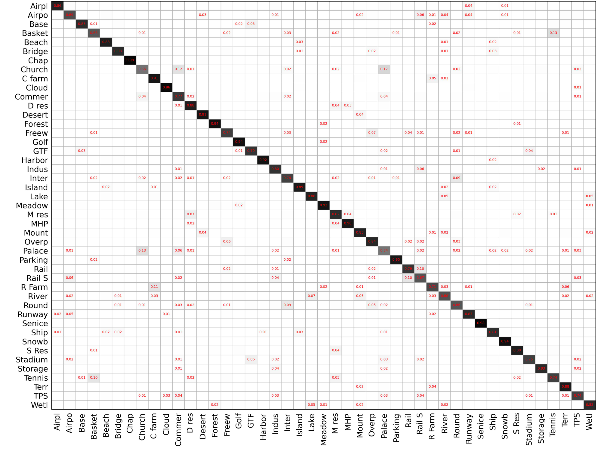
Tables V and VI illustrate the means and standard deviations of OA, AA, and Kappa on AID and NWPU-RESISC45, respectively. For each model, the best performance among different learning schemes (i.e., the models trained from scratch, fine-tuned on ImageNet, and fine-tuned on Million-AID) is reported in bold. By analyzing the tables, one can see that learning directly from scratch achieves the worst result. It indicates that optimizing CNN models for aerial scene classification can be difficult owing to the scarcity of training data and complexity of scene content. Thus, researchers often resort to extracting aerial scene features by models adapted well on natural images and then recognize aerial scenes by utilizing feature classifiers (e.g., SVM [16, 17, 18]). Compared with the models trained from scratch, the models pretrained on ImageNet and Million-AID can significantly improve the classification performance. Figures 8 and 9 provide the confusion matrices of the best results obtained by different learning schemes on AID and NWPU-RESISC45, respectively. It is shown that the classification performance of each scene category is significantly improved by the fine-tuned models. This confirms the importance of parameter initialization for CNN model adaption. In particular, it strongly demonstrates the effectiveness and positive significance of Million-AID for training CNN models toward aerial image scene classification.
An important observation is that all models pretrained on Million-AID achieve obviously better performance compared with those pretrained on ImageNet. Specifically, for both AID and NWPU-RESISC45, each considering CNN model pretrained on Million-AID provides the maximum accuracy. As shown in Figure 8 (b) and (c), by employing Million-AID for model pretraining, the classification accuracy of railway station, center, and airport in AID reach 97%, 88%, and 97%, which are 6%, 4%, and 4% higher than using ImageNet, respectively. Likewise, impressive accuracy improvement can also be observed for scene categories in NWPU-RESISC45, such as golf course, bridge, and intersection as shown in Figure 9 (b) and (c). Figures 10 and 11 provide the corresponding example images and predictions on AID and NWPU-RESISC45, respectively. It is shown that the models pretrained on Million-AID can better distinguish between semantic scenes with similar characteristics. Intuitively, due to the difference in spatial pattern, texture structure, and visual appearance, there are a gigantic feature and semantic discrepancies between the natural and aerial image content. Hence, the CNN models pretrained with natural images may not be generally applicable to reduce this gap for aerial image interpretation. By contrast, the models trained with pure large-scale aerial images can naturally grasp the unique characteristics and knowledge of image content. With this advantage, the subsequent CNN models fine-tuned with aerial images in the target datasets are able to learn better features for aerial scene content representation, and thus, outperform those using the natural images.
From shallow networks (e.g., AlexNet, VGG16, and GoogleNet) to the deeper ones (e.g., ResNet101, DenseNet121, and DenseNet169), the performance difference between ImageNet and Million-AID pretrained models become smaller. As an example on NWPU-RESISC45, AlexNet, VGG16, and GoogleNet pretrained on Million-AID achieves 1.05%, 0.86%, and 1.69% higher OAs than the results from ImageNet pretrained models, respectively. This accuracy difference decreases to 0.14%, 0.31%, and 0.15% when it comes to ResNet101, DenseNet121, and DenseNet169, respectively. The results on AID also show a similar phenomenon. This makes sense because the deeper the network, the more likely the learned features adapted to the target aerial images, resulting in comparable performance among different learning strategies. Nevertheless, the models pretrained with Million-AID still show superiority, which confirms the strong generalization ability of Million-AID. To our knowledge, it is the first time to be observed that CNN models pretrained with pure large-scale aerial images are verified to surpass those using natural images. Prior to this, many CNN models are usually pretrained using the ImageNet dataset and then fine-tuned on the target dataset for aerial image scene classification owing to the lack of available large-scale aerial image archives. With the above observation and results, it is natural to argue that the proposed Million-AID can make an advancement for the use of CNN models in aerial image scene classification, opening up a promising direction to support parameter initialization of CNN models toward various aerial image interpretation tasks such as object detection and semantic segmentation.

V-B Hierarchical multi-task learning for semantic labeling
V-B1 Method of overview
The conventional CNN learns scene features via stacked convolutional layers and the output of the last fully connected layer is usually employed for scene representation. However, learning stable features from a single layer can be a difficult task because of the complexity of scene content. Moreover, data sparsity which is a long-standing notorious problem can easily lead to model overfitting and weak generalization ability because of the insufficient knowledge captured from limited training data. To relieve the above issues, we introduce a hierarchical multi-task learning method and further explore how well the knowledge contained in Million-AID can be transferred to boost the pixel-wise semantic parsing of aerial images. To this end, the GID [8], which consists of a training set with tile-level scenes and large-size test images with pixel-wise annotations, has provided us an opportunity to bridge the tile-level scene classification toward pixel-wise semantic labeling. Generally, the presented framework consists of four components, e.g., hierarchical attention network, multi-task scene classification, hierarchical semantic fusion, and pixel-wise semantics integration, as shown in Figure 12.
Hierarchical attention network (HAN): The high-resolution features from shallow convolutional layers can learn valuable visual information of small objects, texture structures, and spatial patterns associated closely with specific scene content while the semantic clues is insufficient. To compensate for this defect, the hierarchical attention features are learned via transmitting the semantic information from the deep layers to the shallower ones inspired by [202, 203]. Specifically, the deep-layer feature (DF) is firstly upsampled to the same spatial size as the shallow-layer feature (SF) to maintain the semantic information as much as possible. The upsampled semantic feature is processed by a convolutional layer for dimension reduction. And the sigmoid function is then employed to generate the semantic attention map (SAM), which possesses the same channel number as the SF. Element-wise multiplication is conducted between the SF and SAM to generate local attention feature (LAF). Finally, the SF and LAF are assembled by element-wise summation and output the final attention feature (AF). The whole process is illustrated in Figure 13. By repeatably transmitting the deep-layer features to the shallower convolutional layers, we are able to construct the hierarchical attention network (as shown in Figure 12) that incorporates semantic and visual information for scene representation.

Multi-task scene classification (MSC): With the hierarchical attention features, a semantic scene can be represented using the features of multiple scales. As shown in Figure 12, three streams are constructed for multi-scale feature extraction. For each stream, the hierarchical attention feature is further processed by global average pooling and generates the feature for scene representation. Then, the multi-task classification branches are designed to recognize scenes from different datasets. By learning the sharing parameters for different tasks, multi-task learning enables the knowledge learned in one task to be utilized in the others, and thus, improve the generalization ability of a trained model [204, 205]. The presented Million-AID is composed of rich semantic scenes and massive instances that characterize the land cover features. It is reasonable to transfer the land cover knowledge contained in Million-AID to boost the semantic classification of aerial images. With this in mind, the multi-task learning is conducted on Million-AID and the challenging GID [8], which is established for pixel-wise semantic classification of land cover. For simplicity, two branches at each of the hierarchical output layers are designated for the scene-level classification of images in Million-AID and GID, respectively. The summation of weighted losses is used for model adaption:
| (1) | ||||
| (2) | ||||
| (3) |
where represents the cross entropy loss of scene classification using the image features of scale for GID while for Million-AID. indicates the loss weight for the classification at scale . and (where ) indicate the weighted importance of different tasks, i.e., scene classification on GID and Million-AID, respectively. In this work, we aim at improving the classification performance on GID by knowledge transfer from Million-AID. Hence, the semantic classification on GID is regarded as the main task while the scene classification on Million-AID serves as the auxiliary task [206] to still reap the benefits of multi-task learning strategy.
Hierarchical semantic fusion (HSF): To give full play of the advantages of hierarchical attention features, the classification results with different feature scales are integrated. Using the feature at scale , the classification probability vector of image is obtained by a softmax layer:
| (4) |
where represents the probability that belongs to class using the feature of scale . Essentially, the predictions at different scales reflect the probability that a classified scene belongs to individual categories from the perspective of different feature levels. Hence, it is reasonable to integrate the predictions of different scales. To this end, a summation of weighted probabilities is performed as the final prediction:
| (5) |
where indicates the probability that image belongs to class . represents the weight for scale , which serves as the loss weight for the corresponding classification stream. The integration of weighted probabilities aims to provide a more stable prediction result. Then the predicted scene category of image is expressed as:
| (6) |
where is the category label of image .
| GID | Million-AID | ||||||
| Kappa (%) | OA (%) | mIoU (%) | Kappa (%) | OA (%) | AA (%) | ||
| 0.1 | 0.9 | 62.85 | 69.06 | 39.88 | 90.36 | 90.62 | 89.55 |
| 0.3 | 0.7 | 65.15 | 71.00 | 41.85 | 89.44 | 89.72 | 88.91 |
| 0.5 | 0.5 | 66.65 | 72.38 | 42.71 | 89.67 | 89.94 | 89.14 |
| 0.7 | 0.3 | 66.14 | 72.02 | 41.75 | 88.98 | 89.27 | 87.84 |


Pixel-wise semantics integration (PSI): With the above procedures, we can obtain the semantic grid map by tile-level classification for interpreting a large-size aerial image. Here, each semantic grid corresponds to a tile-level classification result. For more accurate results with pixel-wise semantics, the semantic boundaries in an aerial image appear the great importance. We therefore perform class-agnostic image segmentation to produce accurate semantic boundaries. For simplicity, we employ object-based segmentation and a majority voting strategy to generate pixel-wise semantic labeling result. Specifically, the selective search algorithm [207] is conducted on the raw aerial image and produces a homogeneous segmentation map. Let be a homogeneous region in the segmentation map. The majority voting algorithm is then performed to determine the semantic class of denoted as by referencing the semantic grid map:
| (7) |
where denotes the number of pixels enclosed in and labeled as class in the semantic grid map. To enhance the discrimination ability of scene content, we represent the scene with multi-scale context, of which semantic meaning is identified by the central point as illustrated in Figure 1(d). By integrating multi-scale contextual information with tile-level classification, the whole pipeline falls into a hybrid classification framework [8]. Nevertheless, our method focuses more on improving the tile-level scene classification performance by utilizing hierarchical attention features and transferring aerial scene knowledge from the relevant domain, i.e., Million-AID.
V-B2 Implementation detail
ResNet50 [184] is employed as the backbone, where the last three residual blocks of conv3_x, cov4_x, and conv5_x are utilized to extract hierarchical attention features in three streams. The loss weights for the three streams are empirical set to be , , and according to the ratios of channel numbers of the hierarchical layers, respectively. The fine classification set of GID [8], which contains 15 challenging semantic categories, is employed for performance evaluation. Specifically, the proposed model is trained with the subset of 30k tile-level scene patches and then tested on the subset of 10 Gaofen-2 images (68007200) with pixel-wise semantic labels. The multi-scale contextual information is extracted with the windows of 5656, 112112, and 224224, which are consistent with the sizes of training samples. As training samples in GID are highly overlapped, image flipping and rotation (90∘, 180∘, and 270∘) are conducted for data augmentation, resulting in 120k tile-level scene samples. Correspondingly, 120k scene images in Million-AID are randomly selected as the training set, according to the ratios of instance number of each scene category. Training parameters are set the same as those for multi-class scene classification in Section IV except the number of iteration set as 30 epochs. The OA, Kappa, and mean-Intersection-over-Union (mIoU) [149] are employed for performance evaluation.

V-B3 Experimental results
Ablation study: For multi-task learning, the weights of different tasks can make a big influence on the classification performance. Table VII shows the classification result under different weight setups, where the MSC strategy is embedded in the baseline network for tile-level scene classification on Million-AID () and pixel-wise semantic parsing on GID (). Figure 14 illustrates the corresponding changes of training losses with respect to different setups of learning weights. As can be seen, the performance of increases gradually as changes from to . This makes sense because the model tends to optimize when is smaller than . As increases, the model pays incremental attentions to optimize the and borrows knowledge learned from Million-AID concurrently. Particularly, when , the model can be well optimized for , and thus, achieves the best performance with this setup (Figure 14(a)). When , the optimization for is slightly insufficient while gains significant improvement as shown in Figure 14(b). When changes to , both and can be well optimized (Figure 14(c)) and can also benefit from the knowledge learned from GID. Thus, the model gains obvious performance improvement. However, as continues to increase, the performance of both and begin to decline because there is a risk of overfitting for and insufficient optimization for as shown in Figure 14(d). Generally, the best performance for can be acquired when , which is employed in subsequent experiments. As our purpose is to explore the possibility of transferring knowledge in Million-AID to GID for semantic classification of land cover, we will focus on reporting the performance of the main task (i.e., pixel-wise semantic classification on GID) in the following context.
For a better understanding of our presented hierarchical multi-task learning method, detailed ablation studies are conducted with different module settings. Specifically, the ResNet50 is employed as the baseline as introduced before. Then we gradually attach the multi-task scene classification (MSC), hierarchical attention network (HAN), and hierarchical semantic integration (HSF) to the baseline model. Table VIII shows the performance comparison of different setups tested on GID. As can be seen, the results achieved by the baseline is far from satisfactory due to the sparsity of training samples. When employing the MSC strategy, the classification performance reaches 72.38% of OA, 42.71% of mIoU, and 66.65% of Kappa, which are 13.29%, 11.92%, and 15.06% higher than those of baseline, respectively. This strongly verifies the effectiveness of MSC, where diverse scene samples of Million-AID can bring implicit data augmentation and greatly boost the semantic feature learning for GID content representation. Under the circumstances, semantic knowledge contained in Million-AID can be effectively transferred to improve the performance of land cover classification on GID.
When the HAN is introduced, the classification is conducted with the hierarchical features from different streams, respectively. For a scene image, the highest classification score among different streams is adopted to output the corresponding semantic category. As shown in Table VIII, the classification performance is further improved with HAN. This mainly benefits from the hierarchical attention mechanism, where the essential features of a specific scene can be learned within individual layers. With the HSF scheme integrated, the advantage of attention features at different levels is significantly improved and the performance reaches 73.03% of OA, 43.68% of mIoU, and 67.33% of Kappa. As can be seen, the MSC strategy helps most in improving the classification performance while the full implementation of our method achieves the best result.
| Baseline | MSC | HAN | HSF | Kappa (%) | OA (%) | mIoU (%) |
| ✓ | 51.59 | 59.09 | 30.79 | |||
| ✓ | ✓ | 66.65 | 72.38 | 42.71 | ||
| ✓ | ✓ | ✓ | 66.79 | 72.52 | 43.07 | |
| ✓ | ✓ | ✓ | ✓ | 67.33 | 73.03 | 43.68 |
Figure 15 shows the qualitative comparisons of different classification schemes. It is shown that similar categories are easy to be confused by the baseline method. By employing the MSC strategy, many confusing categories can be distinguished, which verifies the effectiveness of the multi-task learning for transferring the scene knowledge contained in Million-AID. With the full implementation of our developed method, the misclassification within some local areas is further corrected, which is consistent with the performance improvement in Table VIII. In general, the designed modules greatly help to grasp the essential semantic knowledge of scene images in Million-AID and GID, thus, improve the generalization ability of the semantic classification model.
Performance comparison: The presented method is compared with several object-based classification methods provided by [8], where four typical features including spectral feature (SF), co-occurrence matrix (GLCM), different morphological profiles (DMP), and local binary patterns (LBP) were fused to obtain the scene representation denoted as SGDL for simplicity. Then, maximum likelihood classification (MLC), random forest (RF), support vector machine (SVM), and multi-layer perception (MLP) are used as classifiers for scene classification, respectively. Besides, we compare our method with the CNN model pretrained on the large-scale classification set of GID (PT-GID) [8]. For comprehensive comparison, the presented method was also compared with the end-to-end semantic segmentation models, such as U-Net [34], PSPNet [199], DeepLab V3+ [208], and its variations like DeepLab V3+ Mixed loss function (DeopLab V3+ MLF), DeepLab v3+ MobileNet provided by [209].
| Methods | Kappa | OA (%) |
| MLC + SGDL | 0.145 | 23.61 |
| SVM + SGDL | 0.148 | 23.92 |
| MLP + SGDL | 0.199 | 30.57 |
| RF + SGDL | 0.237 | 33.70 |
| DeepLab V3+ Mobilenet | 0.357 | 54.64 |
| U-Net | 0.439 | 56.59 |
| PSPNet | 0.458 | 60.73 |
| DeepLab V3+ | 0.478 | 62.19 |
| DeepLab V3+ MLF | 0.598 | 69.16 |
| PT-GID | 0.605 | 70.04 |
| Ours | 0.673 | 73.03 |
The quantitative results of different methods are summarized in Table IX. As can be seen, our method significantly outperforms the object-based ones, showing the superiority of our presented method for semantic content understanding of aerial images. The best result achieved by image segmentation models is 59.8% of Kappa and 69.16% of OA from DeepLab V3+ Mixed Loss Functions (MLF). Note that the segmentation models and its variations are based on fully convolutional networks which learn pixel-wise semantics in an end-to-end way. Nevertheless, our method achieves 7.5% higher Kappa and 3.87% higher OA than those achieved by DeepLab V3+ MLF, indicating the effectiveness of our method for pixel-wise semantic parsing of aerial images. Particularly, PT-GID was achieved by transferring knowledge in the large-scale classification set of GID, which contains 150k samples relevant to the fine classification set of GID. Thus, PT-GID achieves remarkable performance on the fine land-cover classification set. Despite this, our presented method achieves 6.8% higher Kappa and about 3% higher OA, showing the strong transferability and effectiveness of our presented method.

Figure 16 provides the intuitive visualization of the pixel-wise classification results on the fine classification set of GID. To save space, we compare the best two results achieved by PT-GID and our designed method. As can be seen from the first row, the irrigated land is heavily misclassified as dry cropland by PT-GID because of the difficulty in distinguishing their similar visual features, such as the texture and structural information. By contrast, our method can discriminate the irrigated land more accurately even it is widely distributed. This benefits from our hierarchically fused features, which can simultaneously incorporate the visual features and semantic information toward specific scene content. In city areas shown in the second row, many semantic categories, such as the traffic land, urban residential, industrial land, and dry cropland, are heavily confused by PT-GID while our method obtains more accurate classification result. This contributes to the semantic attention feature learning in our method, which helps to grasp the essential information for discriminating content of different categories. Likewise, the extraction of urban residential areas is significantly improved by our method as shown in the third row. On the whole, the classification maps of our method present more homogeneous areas and provide more smoother classification result than those of PT-GID. Thus, our method provide much better classification result than the others, which is consistent with the result in Table IX.
VI Conclusions
In this paper we address aerial scene parsing from tile-level scene classification to pixel-level semantic Labeling. Specifically, a review of aerial image interpretation was firstly conducted from its development perspective. It is shown that the interpretation prototype of aerial images has been progressing with the improvement of image resolution and experienced the stages from pixel-wise image classification, segmentation-based image analysis, and tile-level image understanding. Then, we detailed the large-scale dataset, i.e., Million-AID, to be released for aerial scene recognition. Intensive experiments with popular CNN frameworks indicate that Million-AID is a challenging dataset which can be employed as a benchmark for multi-class and multi-label aerial scene classification. Fine-tuning CNN models pretrained on Million-AID show consistent superiority than those pretrained on ImageNet for aerial scene classification, which demonstrates the strong generalization ability of Million-AID. Besides, we designed a hierarchical multi-task learning framework and achieved the state-of-the-art result for pixel-wise semantic labeling, which is an profitable attempt to bridge the tile-level scene classification toward pixel-wise semantic parsing for aerial image interpretation.
In the future work, we will dedicate our efforts to enrich the Million-AID with more semantic categories and expand the scale of aerial scene images. Knowledge transfer by Million-AID will also be extended to other related tasks, such as object detection and semantic segmentation, to further explore the transferability of Million-AID. We hope that is work can enhance the development of content interpretation algorithms in the field of remote sensing.
References
- [1] M. Weiss, F. Jacob, and G. Duveiller, “Remote sensing for agricultural applications: A meta-review,” Remote Sens. Environ., vol. 236, p. 111402, 2020.
- [2] T. Wellmann, A. Lausch, E. Andersson, S. Knapp, C. Cortinovis, J. Jache, S. Scheuer, P. Kremer, A. Mascarenhas, R. Kraemer et al., “Remote sensing in urban planning: Contributions towards ecologically sound policies?” Landsc. Urban Plan., vol. 204, p. 103921, 2020.
- [3] Q. Yuan, H. Shen, T. Li, Z. Li, S. Li, Y. Jiang, H. Xu, W. Tan, Q. Yang, J. Wang et al., “Deep learning in environmental remote sensing: Achievements and challenges,” Remote Sens. Environ., vol. 241, p. 111716, 2020.
- [4] J. Porway, Q. Wang, and S. C. Zhu, “A hierarchical and contextual model for aerial image parsing,” Int. J. Comput. Vis., vol. 88, no. 2, pp. 254–283, 2010.
- [5] X. Zheng, L. Huan, G.-S. Xia, and J. Gong, “Parsing very high resolution urban scene images by learning deep convnets with edge-aware loss,” ISPRS J. Photogrammetry Remote Sens., vol. 170, pp. 15–28, 2020.
- [6] W. Zhou, J. Jin, J. Lei, and J.-N. Hwang, “CEGFNet: Common extraction and gate fusion network for scene parsing of remote sensing images,” IEEE Trans. Geosci. Remote Sens., pp. 1–10, 2021.
- [7] D. Wang, B. Du, and L. Zhang, “Fully contextual network for hyperspectral scene parsing,” IEEE Trans. Geosci. Remote Sens., vol. 60, pp. 1–16, 2021.
- [8] X.-Y. Tong, G.-S. Xia, Q. Lu, H. Shen, S. Li, S. You, and L. Zhang, “Land-cover classification with high-resolution remote sensing images using transferable deep models,” Remote Sens. Environ., vol. 237, p. 111322, 2020.
- [9] Q. Liu, M. Kampffmeyer, R. Jenssen, and A.-B. Salberg, “Dense dilated convolutions’ merging network for land cover classification,” IEEE Trans. Geosci. Remote Sens., vol. 58, no. 9, pp. 6309–6320, 2020.
- [10] Z. Lv, T. Liu, J. A. Benediktsson, and N. Falco, “Land cover change detection techniques: Very-high-resolution optical images: A review,” IEEE Geosci. Remote Sens. Mag., pp. 2–21, 2021.
- [11] Y. Yang and S. Newsam, “Bag-of-visual-words and spatial extensions for land-use classification,” in Proc. Int. Conf. Adv. Geographic Inf. Syst., 2010, pp. 270–279.
- [12] G. Sheng, W. Yang, T. Xu, and H. Sun, “High-resolution satellite scene classification using a sparse coding based multiple feature combination,” Int. J. Remote Sens., vol. 33, no. 8, pp. 2395–2412, 2012.
- [13] F. Hu, G.-S. Xia, J. Hu, and L. Zhang, “Transferring deep convolutional neural networks for the scene classification of high-resolution remote sensing imagery,” Remote Sens., vol. 7, no. 11, pp. 14 680–14 707, 2015.
- [14] W. Yang, X. Yin, and G.-S. Xia, “Learning high-level features for satellite image classification with limited labeled samples,” IEEE Trans. Geosci. Remote Sens., vol. 53, no. 8, pp. 4472–4482, 2015.
- [15] S. Chen and Y. Tian, “Pyramid of spatial relatons for scene-level land use classification,” IEEE Trans. Geosci. Remote Sens., vol. 53, no. 4, pp. 1947–1957, 2015.
- [16] G.-S. Xia, J. Hu, F. Hu, B. Shi, X. Bai, Y. Zhong, L. Zhang, and X. Lu, “AID: A benchmark data set for performance evaluation of aerial scene classification,” IEEE Trans. Geosci. Remote Sens., vol. 55, no. 7, pp. 3965–3981, 2017.
- [17] G. Cheng, J. Han, and X. Lu, “Remote sensing image scene classification: Benchmark and state of the art,” Proc. IEEE, vol. 105, no. 10, pp. 1865–1883, 2017.
- [18] K. Nogueira, O. A. Penatti, and J. A. dos Santos, “Towards better exploiting convolutional neural networks for remote sensing scene classification,” Pattern Recognit., vol. 61, pp. 539–556, 2017.
- [19] G. Cheng, X. Xie, J. Han, L. Guo, and G.-S. Xia, “Remote sensing image scene classification meets deep learning: Challenges, methods, benchmarks, and opportunities,” IEEE J. Sel. Top. Appl. Earth Obs .Remote Sens., vol. 13, pp. 3735–3756, 2020.
- [20] F. Chen and J. Y. Tsou, “Drsnet: Novel architecture for small patch and low-resolution remote sensing image scene classification,” Int. J. Appl. Earth Obs. Geoinf., vol. 104, p. 102577, 2021.
- [21] A. Sharma, X. Liu, X. Yang, and D. Shi, “A patch-based convolutional neural network for remote sensing image classification,” Neural Netw., vol. 95, pp. 19–28, 2017.
- [22] M. E. Paoletti, J. M. Haut, J. Plaza, and A. Plaza, “A new deep convolutional neural network for fast hyperspectral image classification,” ISPRS J. Photogrammetry Remote Sens., vol. 145, pp. 120–147, 2018.
- [23] A. Sharma, X. Liu, and X. Yang, “Land cover classification from multi-temporal, multi-spectral remotely sensed imagery using patch-based recurrent neural networks,” Neural Netw., vol. 105, pp. 346–355, 2018.
- [24] S. Liu and Q. Shi, “Local climate zone mapping as remote sensing scene classification using deep learning: A case study of metropolitan china,” ISPRS J. Photogrammetry Remote Sens., vol. 164, pp. 229–242, 2020.
- [25] T. Blaschke and J. Strobl, “What’s wrong with pixels? Some recent developments interfacing remote sensing and gis,” GIS-Zeitschrift für Geoinformationssysteme, pp. 12–17, 2001.
- [26] T. Blaschke, “Object based image analysis for remote sensing,” ISPRS J. Photogrammetry Remote Sens., vol. 65, no. 1, pp. 2–16, 2010.
- [27] T. Blaschke, G. J. Hay, M. Kelly, S. Lang, P. Hofmann, E. Addink, R. Q. Feitosa, F. Van der Meer, H. Van der Werff, F. Van Coillie et al., “Geographic object-based image analysis–towards a new paradigm,” ISPRS J. Photogrammetry Remote Sens., vol. 87, pp. 180–191, 2014.
- [28] M. D. Hossain and D. Chen, “Segmentation for object-based image analysis (obia): A review of algorithms and challenges from remote sensing perspective,” ISPRS J. Photogrammetry Remote Sens., vol. 150, pp. 115–134, 2019.
- [29] V. S. Martins, A. L. Kaleita, B. K. Gelder, H. L. da Silveira, and C. A. Abe, “Exploring multiscale object-based convolutional neural network (multi-ocnn) for remote sensing image classification at high spatial resolution,” ISPRS J. Photogrammetry Remote Sens., vol. 168, pp. 56–73, 2020.
- [30] D. Ming, J. Li, J. Wang, and M. Zhang, “Scale parameter selection by spatial statistics for geobia: Using mean-shift based multi-scale segmentation as an example,” ISPRS J. Photogrammetry Remote Sens., vol. 106, pp. 28–41, 2015.
- [31] L. Ma, L. Cheng, M. Li, Y. Liu, and X. Ma, “Training set size, scale, and features in geographic object-based image analysis of very high resolution unmanned aerial vehicle imagery,” ISPRS J. Photogrammetry Remote Sens., vol. 102, pp. 14–27, 2015.
- [32] L. Ma, M. Li, X. Ma, L. Cheng, P. Du, and Y. Liu, “A review of supervised object-based land-cover image classification,” ISPRS J. Photogrammetry Remote Sens., vol. 130, pp. 277–293, 2017.
- [33] J. Long, E. Shelhamer, and T. Darrell, “Fully convolutional networks for semantic segmentation,” in Proc. IEEE Conf. Comput. Vis. Pattern Recognit., 2015, pp. 3431–3440.
- [34] O. Ronneberger, P. Fischer, and T. Brox, “U-Net: Convolutional networks for biomedical image segmentation,” in Proc. Int. Conf. Med. Image Comput. Comput. Assist Interv. Springer, 2015, pp. 234–241.
- [35] V. Badrinarayanan, A. Kendall, and R. Cipolla, “Segnet: A deep convolutional encoder-decoder architecture for image segmentation,” IEEE Trans. Pattern Anal. Mach. Intell., vol. 39, no. 12, pp. 2481–2495, 2017.
- [36] L.-C. Chen, G. Papandreou, I. Kokkinos, K. Murphy, and A. L. Yuille, “Deeplab: Semantic image segmentation with deep convolutional nets, atrous convolution, and fully connected crfs,” IEEE Trans. Pattern Anal. Mach. Intell., vol. 40, no. 4, pp. 834–848, 2017.
- [37] X. X. Zhu, D. Tuia, L. Mou, G.-S. Xia, L. Zhang, F. Xu, and F. Fraundorfer, “Deep learning in remote sensing: A comprehensive review and list of resources,” IEEE Geosci. Remote Sens. Mag., vol. 5, no. 4, pp. 8–36, 2017.
- [38] S. Li, W. Song, L. Fang, Y. Chen, P. Ghamisi, and J. A. Benediktsson, “Deep learning for hyperspectral image classification: An overview,” IEEE Trans. Geosci. Remote Sens., vol. 57, no. 9, pp. 6690–6709, 2019.
- [39] N. Audebert, B. Le Saux, and S. Lefèvre, “Deep learning for classification of hyperspectral data: A comparative review,” IEEE Geosci. Remote Sens. Mag., vol. 7, no. 2, pp. 159–173, 2019.
- [40] K. Yang, X.-Y. Tong, G.-S. Xia, W. Shen, and L. Zhang, “Hidden path selection network for semantic segmentation of remote sensing images,” arXiv preprint arXiv:2112.05220, 2021.
- [41] D. Lu and Q. Weng, “A survey of image classification methods and techniques for improving classification performance,” Int. J. Remote Sens., vol. 28, no. 5, pp. 823–870, 2007.
- [42] C. H. Chen and P.-G. Peter Ho, “Statistical pattern recognition in remote sensing,” Pattern Recognit., vol. 41, no. 9, pp. 2731–2741, 2008.
- [43] D. Tuia, M. Volpi, L. Copa, M. Kanevski, and J. Munoz-Mari, “A survey of active learning algorithms for supervised remote sensing image classification,” IEEE J. Sel. Top. Signal Process., vol. 5, no. 3, pp. 606–617, 2011.
- [44] J. Deng, W. Dong, R. Socher, L. Li, K. Li, and F. Li, “Imagenet: A large-scale hierarchical image database,” in Proc. IEEE Conf. Comput. Vis. Pattern Recognit., 2009, pp. 248–255.
- [45] C. Toth and G. Jóźków, “Remote sensing platforms and sensors: A survey,” ISPRS J. Photogrammetry Remote Sens., vol. 115, pp. 22–36, 2016.
- [46] R. Pu and S. Landry, “A comparative analysis of high spatial resolution ikonos and worldview-2 imagery for mapping urban tree species,” Remote Sens. Environ., vol. 124, pp. 516–533, 2012.
- [47] M. J. Swain and D. H. Ballard, “Color indexing,” Int. J. Comput. Vis., vol. 7, no. 1, pp. 11–32, 1991.
- [48] T. Ojala, M. Pietikainen, and T. Maenpaa, “Multiresolution gray-scale and rotation invariant texture classification with local binary patterns,” IEEE Trans. Pattern Anal. Mach. Intell., vol. 24, no. 7, pp. 971–987, 2002.
- [49] R. M. Haralick, K. Shanmugam, and I. H. Dinstein, “Textural features for image classification,” IEEE Trans. Syst. Man. Cybern. Syst., no. 6, pp. 610–621, 1973.
- [50] B. S. Manjunath and W.-Y. Ma, “Texture features for browsing and retrieval of image data,” IEEE Trans. Pattern Anal. Mach. Intell., vol. 18, no. 8, pp. 837–842, 1996.
- [51] T. Ojala, M. Pietikäinen, and T. Mäenpää, “Gray scale and rotation invariant texture classification with local binary patterns,” in Proc. Eur. Conf. Comput. Vis., 2000, pp. 404–420.
- [52] G.-S. Xia, J. Delon, and Y. Gousseau, “Shape-based invariant texture indexing,” Int. J. Comput. Vis., vol. 88, no. 3, pp. 382–403, 2010.
- [53] J. Van Genderen, B. Lock, and P. Vass, “Remote sensing: Statistical testing of thematic map accuracy,” Remote Sens. Environ., vol. 7, no. 1, pp. 3–14, 1978.
- [54] P. Curran and H. Williamson, “Sample size for ground and remotely sensed data,” Remote Sens. Environ., vol. 20, no. 1, pp. 31–41, 1986.
- [55] R. Khatami, G. Mountrakis, and S. V. Stehman, “Mapping per-pixel predicted accuracy of classified remote sensing images,” Remote Sens. Environ., vol. 191, pp. 156–167, 2017.
- [56] L. Bruzzone, D. F. Prieto, and S. B. Serpico, “A neural-statistical approach to multitemporal and multisource remote-sensing image classification,” IEEE Trans. Geosci. Remote Sens., vol. 37, no. 3, pp. 1350–1359, 1999.
- [57] J. Li, J. M. Bioucas-Dias, and A. Plaza, “Semisupervised hyperspectral image segmentation using multinomial logistic regression with active learning,” IEEE Trans. Geosci. Remote Sens., vol. 48, no. 11, pp. 4085–4098, 2010.
- [58] G. Camps-Valls, D. Tuia, L. Bruzzone, and J. A. Benediktsson, “Advances in hyperspectral image classification: Earth monitoring with statistical learning methods,” IEEE Signal Process. Mag., vol. 31, no. 1, pp. 45–54, 2013.
- [59] J. Li, J. M. Bioucas-Dias, and A. Plaza, “Hyperspectral image segmentation using a new bayesian approach with active learning,” IEEE Trans. Geosci. Remote Sens., vol. 49, no. 10, pp. 3947–3960, 2011.
- [60] J. Zhao, Y. Zhong, H. Shu, and L. Zhang, “High-resolution image classification integrating spectral-spatial-location cues by conditional random fields,” IEEE Trans. Image Process., vol. 25, no. 9, pp. 4033–4045, 2016.
- [61] J. Settle and S. Briggs, “Fast maximum likelihood classification of remotely-sensed imagery,” Int. J. Remote Sens., vol. 8, no. 5, pp. 723–734, 1987.
- [62] J. Ediriwickrema and S. Khorram, “Hierarchical maximum-likelihood classification for improved accuracies,” IEEE Trans. Geosci. Remote Sens., vol. 35, no. 4, pp. 810–816, 1997.
- [63] J. Peng, L. Li, and Y. Y. Tang, “Maximum likelihood estimation-based joint sparse representation for the classification of hyperspectral remote sensing images,” IEEE Trans. Neural Netw. Learn. Syst., vol. 30, no. 6, pp. 1790–1802, 2019.
- [64] M. E. Hodgson, “Reducing the computational requirements of the minimum-distance classifier,” Remote Sens. Environ., vol. 25, no. 1, pp. 117–128, 1988.
- [65] M. Espínola, J. A. Piedra-Fernández, R. Ayala, L. Iribarne, and J. Z. Wang, “Contextual and hierarchical classification of satellite images based on cellular automata,” IEEE Trans. Geosci. Remote Sens., vol. 53, no. 2, pp. 795–809, 2014.
- [66] L. Ma, M. M. Crawford, and J. Tian, “Local manifold learning-based -nearest-neighbor for hyperspectral image classification,” IEEE Trans. Geosci. Remote Sens., vol. 48, no. 11, pp. 4099–4109, 2010.
- [67] B. Tu, S. Huang, L. Fang, G. Zhang, J. Wang, and B. Zheng, “Hyperspectral image classification via weighted joint nearest neighbor and sparse representation,” IEEE J. Sel. Top. Appl. Earth Obs. Remote Sens., vol. 11, no. 11, pp. 4063–4075, 2018.
- [68] M. A. Friedl and C. E. Brodley, “Decision tree classification of land cover from remotely sensed data,” Remote Sens. Environ., vol. 61, no. 3, pp. 399–409, 1997.
- [69] J. R. Otukei and T. Blaschke, “Land cover change assessment using decision trees, support vector machines and maximum likelihood classification algorithms,” Int. J. Appl. Earth Obs. Geoinf., vol. 12, pp. S27–S31, 2010.
- [70] M. Belgiu and L. Drăguţ, “Random forest in remote sensing: A review of applications and future directions,” ISPRS J. Photogrammetry Remote Sens., vol. 114, pp. 24–31, 2016.
- [71] J. Xia, P. Ghamisi, N. Yokoya, and A. Iwasaki, “Random forest ensembles and extended multiextinction profiles for hyperspectral image classification,” IEEE Trans. Geosci. Remote Sens., vol. 56, no. 1, pp. 202–216, 2018.
- [72] E. Izquierdo-Verdiguier and R. Zurita-Milla, “An evaluation of guided regularized random forest for classification and regression tasks in remote sensing,” Int. J. Appl. Earth Obs. Geoinf., vol. 88, p. 102051, 2020.
- [73] A. Zafari, R. Zurita-Milla, and E. Izquierdo-Verdiguier, “A multiscale random forest kernel for land cover classification,” IEEE J. Sel. Top. Appl. Earth Obs. Remote Sens., vol. 13, pp. 2842–2852, 2020.
- [74] H. Lee, A. Battle, R. Raina, and A. Y. Ng, “Efficient sparse coding algorithms,” in Adv. Neural Inf. Process. Syst., 2007, pp. 801–808.
- [75] J. Liu, Z. Wu, Z. Wei, L. Xiao, and L. Sun, “Spatial-spectral kernel sparse representation for hyperspectral image classification,” IEEE J. Sel. Top. Appl. Earth Obs. Remote Sens., vol. 6, no. 6, pp. 2462–2471, 2013.
- [76] Z. Feng, M. Wang, S. Yang, Z. Liu, L. Liu, B. Wu, and H. Li, “Superpixel tensor sparse coding for structural hyperspectral image classification,” IEEE J. Sel. Top. Appl. Earth Obs. Remote Sens., vol. 10, no. 4, pp. 1632–1639, 2017.
- [77] J. Fan, T. Chen, and S. Lu, “Superpixel guided deep-sparse-representation learning for hyperspectral image classification,” IEEE Trans. Circuits Syst. Video Technol., vol. 28, no. 11, pp. 3163–3173, 2017.
- [78] D. Li, Q. Wang, and F. Kong, “Adaptive kernel sparse representation based on multiple feature learning for hyperspectral image classification,” Neurocomputing, vol. 400, pp. 97–112, 2020.
- [79] T. Kavzoglu and P. Mather, “The use of backpropagating artificial neural networks in land cover classification,” Int. J. Remote Sens., vol. 24, no. 23, pp. 4907–4938, 2003.
- [80] Y. Shao and R. S. Lunetta, “Comparison of support vector machine, neural network, and cart algorithms for the land-cover classification using limited training data points,” ISPRS J. Photogrammetry Remote Sens., vol. 70, pp. 78–87, 2012.
- [81] Y. Gu, J. Chanussot, X. Jia, and J. A. Benediktsson, “Multiple kernel learning for hyperspectral image classification: A review,” IEEE Trans. Geosci. Remote Sens., vol. 55, no. 11, pp. 6547–6565, 2017.
- [82] G. Mountrakis, J. Im, and C. Ogole, “Support vector machines in remote sensing: A review,” ISPRS J. Photogrammetry Remote Sens., vol. 66, no. 3, pp. 247–259, 2011.
- [83] U. Maulik and D. Chakraborty, “Remote sensing image classification: A survey of support-vector-machine-based advanced techniques,” IEEE Geosci. Remote Sens. Mag., vol. 5, no. 1, pp. 33–52, 2017.
- [84] O. Okwuashi and C. E. Ndehedehe, “Deep support vector machine for hyperspectral image classification,” Pattern Recognit., vol. 103, p. 107298, 2020.
- [85] M. Li, S. Zang, B. Zhang, S. Li, and C. Wu, “A review of remote sensing image classification techniques: The role of spatio-contextual information,” Eur. J. Remote Sens., vol. 47, no. 1, pp. 389–411, 2014.
- [86] W. Liu and E. Y. Wu, “Comparison of non-linear mixture models: sub-pixel classification,” Remote Sens. Environ., vol. 94, no. 2, pp. 145–154, 2005.
- [87] F. Bovolo, L. Bruzzone, and L. Carlin, “A novel technique for subpixel image classification based on support vector machine,” IEEE Trans. Image Process., vol. 19, no. 11, pp. 2983–2999, 2010.
- [88] Q. Wang, C. Zhang, and P. M. Atkinson, “Sub-pixel mapping with point constraints,” Remote Sens. Environ., vol. 244, p. 111817, 2020.
- [89] D. He, Q. Shi, X. Liu, Y. Zhong, and X. Zhang, “Deep subpixel mapping based on semantic information modulated network for urban land use mapping,” IEEE Trans. Geosci. Remote Sens., vol. 59, no. 12, pp. 10 628–10 646, 2021.
- [90] F. Wang, “Fuzzy supervised classification of remote sensing images,” IEEE Trans. Geosci. Remote Sens., vol. 28, no. 2, pp. 194–201, 1990.
- [91] A. K. Shackelford and C. H. Davis, “A hierarchical fuzzy classification approach for high-resolution multispectral data over urban areas,” IEEE Trans. Geosci. Remote Sens., vol. 41, no. 9, pp. 1920–1932, 2003.
- [92] N. S. Kothari, S. K. Meher, and G. Panda, “Improved spatial information based semisupervised classification of remote sensing images,” IEEE J. Sel. Top. Appl. Earth Obs. Remote Sens., vol. 13, pp. 329–340, 2020.
- [93] K. C. Mertens, L. P. Verbeke, T. Westra, and R. R. De Wulf, “Sub-pixel mapping and sub-pixel sharpening using neural network predicted wavelet coefficients,” Remote Sens. Environ., vol. 91, no. 2, pp. 225–236, 2004.
- [94] X. Li, F. Ling, Y. Du, Q. Feng, and Y. Zhang, “A spatial–temporal hopfield neural network approach for super-resolution land cover mapping with multi-temporal different resolution remotely sensed images,” ISPRS J. Photogrammetry Remote Sens., vol. 93, pp. 76–87, 2014.
- [95] D. He, Y. Zhong, X. Wang, and L. Zhang, “Deep convolutional neural network framework for subpixel mapping,” IEEE Trans. Geosci. Remote Sens., vol. 59, no. 11, pp. 9518–9539, 2020.
- [96] R. Fernandes, R. Fraser, R. Latifovic, J. Cihlar, J. Beaubien, and Y. Du, “Approaches to fractional land cover and continuous field mapping: A comparative assessment over the boreas study region,” Remote Sens. Environ., vol. 89, no. 2, pp. 234–251, 2004.
- [97] U. Gessner, M. Machwitz, C. Conrad, and S. Dech, “Estimating the fractional cover of growth forms and bare surface in savannas. a multi-resolution approach based on regression tree ensembles,” Remote Sens. Environ., vol. 129, pp. 90–102, 2013.
- [98] S. Cooper, A. Okujeni, C. Jänicke, M. Clark, S. van der Linden, and P. Hostert, “Disentangling fractional vegetation cover: Regression-based unmixing of simulated spaceborne imaging spectroscopy data,” Remote Sens. Environ., vol. 246, p. 111856, 2020.
- [99] C. Wu and A. T. Murray, “Estimating impervious surface distribution by spectral mixture analysis,” Remote Sens. Environ., vol. 84, no. 4, pp. 493–505, 2003.
- [100] B. Somers, G. P. Asner, L. Tits, and P. Coppin, “Endmember variability in spectral mixture analysis: A review,” Remote Sens. Environ., vol. 115, no. 7, pp. 1603–1616, 2011.
- [101] J. Yu, B. Wang, Y. Lin, F. Li, and J. Cai, “A novel inequality-constrained weighted linear mixture model for endmember variability,” Remote Sens. Environ., vol. 257, p. 112359, 2021.
- [102] F. Xu and B. Somers, “Unmixing-based sentinel-2 downscaling for urban land cover mapping,” ISPRS J. Photogrammetry Remote Sens., vol. 171, pp. 133–154, 2021.
- [103] A. Bateson and B. Curtiss, “A method for manual endmember selection and spectral unmixing,” Remote Sens. Environ., vol. 55, no. 3, pp. 229–243, 1996.
- [104] C. Small, “The landsat etm+ spectral mixing space,” Remote Sens. Environ., vol. 93, no. 1-2, pp. 1–17, 2004.
- [105] S. Ozkan, B. Kaya, and G. B. Akar, “EndNet: Sparse autoencoder network for endmember extraction and hyperspectral unmixing,” IEEE Trans. Geosci. Remote Sens., vol. 57, no. 1, pp. 482–496, 2019.
- [106] D. Hong, L. Gao, J. Yao, N. Yokoya, J. Chanussot, U. Heiden, and B. Zhang, “Endmember-guided unmixing network (egu-net): A general deep learning framework for self-supervised hyperspectral unmixing,” IEEE Trans. Neural Netw. Learn. Syst., pp. 1–14, 2021.
- [107] P. M. Atkinson, “Mapping sub-pixel boundaries from remotely sensed images,” in Innovations in GIS, 1997, pp. 184–202.
- [108] Q. Wang and P. M. Atkinson, “The effect of the point spread function on sub-pixel mapping,” Remote Sens. Environ., vol. 193, pp. 127–137, 2017.
- [109] G. J. Hay and G. Castilla, “Geographic object-based image analysis (geobia): A new name for a new discipline,” in Object-based Image Analysis. Springer, 2008, pp. 75–89.
- [110] I. Kotaridis and M. Lazaridou, “Remote sensing image segmentation advances: A meta-analysis,” ISPRS J. Photogrammetry Remote Sens., vol. 173, pp. 309–322, 2021.
- [111] G. Hay, D. Marceau, P. Dube, and A. Bouchard, “A multiscale framework for landscape analysis: object-specific analysis and upscaling,” Landsc Ecol., vol. 16, no. 6, pp. 471–490, 2001.
- [112] H.-D. Cheng, X. H. Jiang, Y. Sun, and J. Wang, “Color image segmentation: advances and prospects,” Pattern Recognit., vol. 34, no. 12, pp. 2259–2281, 2001.
- [113] T. R. Martha, N. Kerle, C. J. van Westen, V. Jetten, and K. V. Kumar, “Segment optimization and data-driven thresholding for knowledge-based landslide detection by object-based image analysis,” IEEE Trans. Geosci. Remote Sens., vol. 49, no. 12, pp. 4928–4943, 2011.
- [114] J. Yang, Y. He, and J. Caspersen, “Region merging using local spectral angle thresholds: A more accurate method for hybrid segmentation of remote sensing images,” Remote Sens. Environ., vol. 190, pp. 137–148, 2017.
- [115] Y. Tang, F. Qiu, L. Jing, F. Shi, and X. Li, “Integrating spectral variability and spatial distribution for object-based image analysis using curve matching approaches,” ISPRS J. Photogrammetry Remote Sens., vol. 169, pp. 320–336, 2020.
- [116] D. Amitrano, F. Cecinati, G. Di Martino, A. Iodice, P.-P. Mathieu, D. Riccio, and G. Ruello, “Feature extraction from multitemporal sar images using selforganizing map clustering and object-based image analysis,” IEEE J. Sel. Top. Appl. Earth Obs. Remote Sens., vol. 11, no. 5, pp. 1556–1570, 2018.
- [117] B. Kaur and A. Garg, “Mathematical morphological edge detection for remote sensing images,” in Proc. Int. Conf. Electron. Comput. Technol., vol. 5, 2011, pp. 324–327.
- [118] X. Han, X. Huang, J. Li, Y. Li, M. Y. Yang, and J. Gong, “The edge-preservation multi-classifier relearning framework for the classification of high-resolution remotely sensed imagery,” ISPRS J. Photogrammetry Remote Sens., vol. 138, pp. 57–73, 2018.
- [119] R. Shang, M. Liu, J. Lin, J. Feng, Y. Li, R. Stolkin, and L. Jiao, “Sar image segmentation based on constrained smoothing and hierarchical label correction,” IEEE Trans. Geosci. Remote Sens., pp. 1–16, 2021.
- [120] J. Liu, P. Li, and X. Wang, “A new segmentation method for very high resolution imagery using spectral and morphological information,” ISPRS J. Photogrammetry Remote Sens., vol. 101, pp. 145–162, 2015.
- [121] T. Su, “Scale-variable region-merging for high resolution remote sensing image segmentation,” ISPRS J. Photogrammetry Remote Sens., vol. 147, pp. 319–334, 2019.
- [122] T. Su, T. Liu, S. Zhang, Z. Qu, and R. Li, “Machine learning-assisted region merging for remote sensing image segmentation,” ISPRS J. Photogrammetry Remote Sens., vol. 168, pp. 89–123, 2020.
- [123] X. Zhang, P. Xiao, X. Feng, J. Wang, and Z. Wang, “Hybrid region merging method for segmentation of high-resolution remote sensing images,” ISPRS J. Photogrammetry Remote Sens., vol. 98, pp. 19–28, 2014.
- [124] R. Niu, X. Sun, Y. Tian, W. Diao, K. Chen, and K. Fu, “Hybrid multiple attention network for semantic segmentation in aerial images,” IEEE Trans. Geosci. Remote Sens., vol. 60, pp. 1–18, 2021.
- [125] P. Ghamisi, J. Plaza, Y. Chen, J. Li, and A. J. Plaza, “Advanced spectral classifiers for hyperspectral images: A review,” IEEE Geosci. Remote Sens. Mag., vol. 5, no. 1, pp. 8–32, 2017.
- [126] B. Kumar, O. Dikshit, A. Gupta, and M. K. Singh, “Feature extraction for hyperspectral image classification: a review,” Int. J. Remote Sens., vol. 41, no. 16, pp. 6248–6287, 2020.
- [127] C. Zhang, I. Sargent, X. Pan, H. Li, A. Gardiner, J. Hare, and P. M. Atkinson, “An object-based convolutional neural network (ocnn) for urban land use classification,” Remote Sens. Environ., vol. 216, pp. 57–70, 2018.
- [128] C. Zhang, P. Yue, D. Tapete, B. Shangguan, M. Wang, and Z. Wu, “A multi-level context-guided classification method with object-based convolutional neural network for land cover classification using very high resolution remote sensing images,” Int. J. Appl. Earth Obs. Geoinf., vol. 88, p. 102086, 2020.
- [129] E. Maggiori, Y. Tarabalka, G. Charpiat, and P. Alliez, “Convolutional neural networks for large-scale remote-sensing image classification,” IEEE Trans. Geosci. Remote Sens., vol. 55, no. 2, pp. 645–657, 2016.
- [130] S. Jia, S. Jiang, Z. Lin, N. Li, M. Xu, and S. Yu, “A survey: Deep learning for hyperspectral image classification with few labeled samples,” Neurocomputing, vol. 448, pp. 179–204, 2021.
- [131] C. Zhang, G. Li, and S. Du, “Multi-scale dense networks for hyperspectral remote sensing image classification,” IEEE Trans. Geosci. Remote Sens., vol. 57, no. 11, pp. 9201–9222, 2019.
- [132] K. Yang, Z. Liu, Q. Lu, and G.-S. Xia, “Multi-scale weighted branch network for remote sensing image classification,” in Proc. IEEE Conf. Comput. Vis. Pattern Recognit. Workshops, 2019, pp. 1–10.
- [133] C. Peng, Y. Li, L. Jiao, Y. Chen, and R. Shang, “Densely based multi-scale and multi-modal fully convolutional networks for high-resolution remote-sensing image semantic segmentation,” IEEE J. Sel. Top. Appl. Earth Obs. Remote Sens., vol. 12, no. 8, pp. 2612–2626, 2019.
- [134] G. Sun, X. Zhang, X. Jia, J. Ren, A. Zhang, Y. Yao, and H. Zhao, “Deep fusion of localized spectral features and multi-scale spatial features for effective classification of hyperspectral images,” Int. J. Appl. Earth Obs. Geoinf., vol. 91, p. 102157, 2020.
- [135] M. Zhang, W. Li, and Q. Du, “Diverse region-based cnn for hyperspectral image classification,” IEEE Trans. Image Process., vol. 27, no. 6, pp. 2623–2634, 2018.
- [136] Z. Niu, W. Liu, J. Zhao, and G. Jiang, “Deeplab-based spatial feature extraction for hyperspectral image classification,” IEEE Geosci. Remote Sens. Lett., vol. 16, no. 2, pp. 251–255, 2018.
- [137] L. He, J. Li, C. Liu, and S. Li, “Recent advances on spectral–spatial hyperspectral image classification: An overview and new guidelines,” IEEE Trans. Geosci. Remote Sens., vol. 56, no. 3, pp. 1579–1597, 2017.
- [138] P. Ghamisi, E. Maggiori, S. Li, R. Souza, Y. Tarablaka, G. Moser, A. De Giorgi, L. Fang, Y. Chen, M. Chi et al., “New frontiers in spectral-spatial hyperspectral image classification: The latest advances based on mathematical morphology, markov random fields, segmentation, sparse representation, and deep learning,” IEEE Geosci. Remote Sens. Mag., vol. 6, no. 3, pp. 10–43, 2018.
- [139] Q. Gao, S. Lim, and X. Jia, “Spectral–spatial hyperspectral image classification using a multiscale conservative smoothing scheme and adaptive sparse representation,” IEEE Trans. Geosci. Remote Sens., vol. 57, no. 10, pp. 7718–7730, 2019.
- [140] L. Mou and X. X. Zhu, “Learning to pay attention on spectral domain: A spectral attention module-based convolutional network for hyperspectral image classification,” IEEE Trans. Geosci. Remote Sens., vol. 58, no. 1, pp. 110–122, 2019.
- [141] J. Feng, J. Chen, L. Liu, X. Cao, X. Zhang, L. Jiao, and T. Yu, “CNN-based multilayer spatial–spectral feature fusion and sample augmentation with local and nonlocal constraints for hyperspectral image classification,” IEEE J. Sel. Top. Appl. Earth Obs. Remote Sens., vol. 12, no. 4, pp. 1299–1313, 2019.
- [142] Z. Li, T. Wang, W. Li, Q. Du, C. Wang, C. Liu, and X. Shi, “Deep multilayer fusion dense network for hyperspectral image classification,” IEEE J. Sel. Top. Appl. Earth Obs. Remote Sens., vol. 13, pp. 1258–1270, 2020.
- [143] M. Imani and H. Ghassemian, “An overview on spectral and spatial information fusion for hyperspectral image classification: Current trends and challenges,” Inf. Fusion, vol. 59, pp. 59–83, 2020.
- [144] M. Wurm, T. Stark, X. X. Zhu, M. Weigand, and H. Taubenböck, “Semantic segmentation of slums in satellite images using transfer learning on fully convolutional neural networks,” ISPRS J. Photogrammetry Remote Sens., vol. 150, pp. 59–69, 2019.
- [145] Y. Chen, Y. Wang, Y. Gu, X. He, P. Ghamisi, and X. Jia, “Deep learning ensemble for hyperspectral image classification,” IEEE J. Sel. Top. Appl. Earth Obs. Remote Sens., vol. 12, no. 6, pp. 1882–1897, 2019.
- [146] X. He and Y. Chen, “Transferring cnn ensemble for hyperspectral image classification,” IEEE Geosci. Remote Sens. Lett., vol. 18, no. 5, pp. 876–880, 2020.
- [147] L. Ma, Y. Liu, X. Zhang, Y. Ye, G. Yin, and B. A. Johnson, “Deep learning in remote sensing applications: A meta-analysis and review,” ISPRS J. Photogrammetry Remote Sens., vol. 152, pp. 166–177, 2019.
- [148] F. Lateef and Y. Ruichek, “Survey on semantic segmentation using deep learning techniques,” Neurocomputing, vol. 338, pp. 321–348, 2019.
- [149] S. Minaee, Y. Y. Boykov, F. Porikli, A. J. Plaza, N. Kehtarnavaz, and D. Terzopoulos, “Image segmentation using deep learning: A survey,” IEEE Trans. Pattern Anal. Mach. Intell., 2021.
- [150] G.-S. Xia, W. Yang, J. Delon, Y. Gousseau, H. Sun, and H. Maître, “Structural high-resolution satellite image indexing,” in Proc. ISPRS TC VII Symposium - 100 Years ISPRS, 2010, pp. 298–303.
- [151] Y. Zhong, Q. Zhu, and L. Zhang, “Scene classification based on the multifeature fusion probabilistic topic model for high spatial resolution remote sensing imagery,” IEEE Trans. Geosci. Remote Sens., vol. 53, no. 11, pp. 6207–6222, 2015.
- [152] E. Li, J. Xia, P. Du, C. Lin, and A. Samat, “Integrating multilayer features of convolutional neural networks for remote sensing scene classification,” IEEE Trans. Geosci. Remote Sens., vol. 55, no. 10, pp. 5653–5665, 2017.
- [153] N. He, L. Fang, S. Li, A. Plaza, and J. Plaza, “Remote sensing scene classification using multilayer stacked covariance pooling,” IEEE Trans. Geosci. Remote Sens., vol. 56, no. 12, pp. 6899–6910, 2018.
- [154] S. Chaib, H. Liu, Y. Gu, and H. Yao, “Deep feature fusion for vhr remote sensing scene classification,” IEEE Trans. Geosci. Remote Sens., vol. 55, no. 8, pp. 4775–4784, 2017.
- [155] A. Raza, H. Huo, S. Sirajuddin, and T. Fang, “Diverse capsules network combining multiconvolutional layers for remote sensing image scene classification,” IEEE J. Sel. Top. Appl. Earth Obs. Remote Sens., vol. 13, pp. 5297–5313, 2020.
- [156] Q. Bi, H. Zhang, and K. Qin, “Multi-scale stacking attention pooling for remote sensing scene classification,” Neurocomputing, vol. 436, pp. 147–161, 2021.
- [157] Y. Yuan, J. Fang, X. Lu, and Y. Feng, “Remote sensing image scene classification using rearranged local features,” IEEE Trans. Geosci. Remote Sens., vol. 57, no. 3, pp. 1779–1792, 2019.
- [158] Q. Bi, K. Qin, H. Zhang, and G.-S. Xia, “Local semantic enhanced convnet for aerial scene recognition,” IEEE Trans. Image Process., vol. 30, pp. 6498–6511, 2021.
- [159] Q. Bi, B. Zhou, W. Ji, K. Qin, Q. Ye, and G.-S. Xia., “All grains, one scheme (AGOS): Learning multi-grain instance representation for aerial scene classification,” IEEE Trans. Image Process., pp. 1–15, 2022.
- [160] Q. Wang, S. Liu, J. Chanussot, and X. Li, “Scene classification with recurrent attention of vhr remote sensing images,” IEEE Trans. Geosci. Remote Sens., vol. 57, no. 2, pp. 1155–1167, 2019.
- [161] Q. Bi, K. Qin, Z. Li, H. Zhang, K. Xu, and G.-S. Xia, “A multiple-instance densely-connected convnet for aerial scene classification,” IEEE Trans. Image Process., vol. 29, pp. 4911–4926, 2020.
- [162] L. Fu, D. Zhang, and Q. Ye, “Recurrent thrifty attention network for remote sensing scene recognition,” IEEE Trans. Geosci. Remote Sens., vol. 59, no. 10, pp. 8257–8268, 2020.
- [163] G. Cheng, C. Yang, X. Yao, L. Guo, and J. Han, “When deep learning meets metric learning: Remote sensing image scene classification via learning discriminative cnns,” IEEE Trans. Geosci. Remote Sens., vol. 56, no. 5, pp. 2811–2821, 2018.
- [164] Z. Gong, P. Zhong, Y. Yu, and W. Hu, “Diversity-promoting deep structural metric learning for remote sensing scene classification,” IEEE Trans. Geosci. Remote Sens., vol. 56, no. 1, pp. 371–390, 2018.
- [165] J. Kang, R. Fernandez-Beltran, Z. Ye, X. Tong, P. Ghamisi, and A. Plaza, “Deep metric learning based on scalable neighborhood components for remote sensing scene characterization,” IEEE Trans. Geosci. Remote Sens., vol. 58, no. 12, pp. 8905–8918, 2020.
- [166] Y. Wang, L. Zhang, X. Tong, F. Nie, H. Huang, and J. Mei, “LRAGE: Learning latent relationships with adaptive graph embedding for aerial scene classification,” IEEE Trans. Geosci. Remote Sens., vol. 56, no. 2, pp. 621–634, 2018.
- [167] N. Khan, U. Chaudhuri, B. Banerjee, and S. Chaudhuri, “Graph convolutional network for multi-label vhr remote sensing scene recognition,” Neurocomputing, vol. 357, pp. 36–46, 2019.
- [168] J. Kang, R. Fernandez-Beltran, D. Hong, J. Chanussot, and A. Plaza, “Graph relation network: Modeling relations between scenes for multilabel remote-sensing image classification and retrieval,” IEEE Trans. Geosci. Remote Sens., vol. 59, no. 5, pp. 4355–4369, 2021.
- [169] A. Ma, Y. Wan, Y. Zhong, J. Wang, and L. Zhang, “Scenenet: Remote sensing scene classification deep learning network using multi-objective neural evolution architecture search,” ISPRS J. Photogrammetry Remote Sens., vol. 172, pp. 171–188, 2021.
- [170] C. Peng, Y. Li, L. Jiao, and R. Shang, “Efficient convolutional neural architecture search for remote sensing image scene classification,” IEEE Trans. Geosci. Remote Sens., vol. 59, no. 7, pp. 6092–6105, 2021.
- [171] C. Broni-Bediako, Y. Murata, L. H. B. Mormille, and M. Atsumi, “Searching for cnn architectures for remote sensing scene classification,” IEEE Trans. Geosci. Remote Sens., pp. 1–13, 2021.
- [172] G. Cheng, L. Cai, C. Lang, X. Yao, J. Chen, L. Guo, and J. Han, “SPNet: Siamese-prototype network for few-shot remote sensing image scene classification,” IEEE Trans. Geosci. Remote Sens., pp. 1–11, 2021.
- [173] H. Li, Z. Cui, Z. Zhu, L. Chen, J. Zhu, H. Huang, and C. Tao, “Rs-metanet: Deep metametric learning for few-shot remote sensing scene classification,” IEEE Trans. Geosci. Remote Sens., vol. 59, no. 8, pp. 6983–6994, 2021.
- [174] Y. Liu, L. Zhang, Z. Han, and C. Chen, “Integrating knowledge distillation with learning to rank for few-shot scene classification,” IEEE Trans. Geosci. Remote Sens., pp. 1–12, 2021.
- [175] E. Othman, Y. Bazi, F. Melgani, H. Alhichri, N. Alajlan, and M. Zuair, “Domain adaptation network for cross-scene classification,” IEEE Trans. Geosci. Remote Sens., vol. 55, no. 8, pp. 4441–4456, 2017.
- [176] X. Lu, T. Gong, and X. Zheng, “Multisource compensation network for remote sensing cross-domain scene classification,” IEEE Trans. Geosci. Remote Sens., vol. 58, no. 4, pp. 2504–2515, 2020.
- [177] J. Zhang, J. Liu, B. Pan, and Z. Shi, “Domain adaptation based on correlation subspace dynamic distribution alignment for remote sensing image scene classification,” IEEE Trans. Geosci. Remote Sens., vol. 58, no. 11, pp. 7920–7930, 2020.
- [178] S. Zhu, B. Du, L. Zhang, and X. Li, “Attention-based multiscale residual adaptation network for cross-scene classification,” IEEE Trans. Geosci. Remote Sens., pp. 1–15, 2021.
- [179] Y. Long, G.-S. Xia, S. Li, W. Yang, M. Y. Yang, X. X. Zhu, L. Zhang, and D. Li, “On creating benchmark dataset for aerial image interpretation: Reviews, guidances, and million-aid,” IEEE J. Sel. Top. Appl. Earth Obs. Remote Sens., vol. 14, pp. 4205–4230, 2021.
- [180] M. Reichstein, G. Camps-Valls, B. Stevens, M. Jung, J. Denzler, N. Carvalhais et al., “Deep learning and process understanding for data-driven earth system science,” Nature, vol. 566, no. 7743, pp. 195–204, 2019.
- [181] A. Krizhevsky, I. Sutskever, and G. E. Hinton, “Imagenet classification with deep convolutional neural networks,” Adv. Neural Inf. Process. Syst., vol. 25, pp. 1097–1105, 2012.
- [182] K. Simonyan and A. Zisserman, “Very deep convolutional networks for large-scale image recognition,” arXiv preprint arXiv:1409.1556, 2014.
- [183] C. Szegedy, W. Liu, Y. Jia, P. Sermanet, S. Reed, D. Anguelov, D. Erhan, V. Vanhoucke, and A. Rabinovich, “Going deeper with convolutions,” in Proc. IEEE Conf. Comput. Vis. Pattern Recognit., 2015, pp. 1–9.
- [184] K. He, X. Zhang, S. Ren, and J. Sun, “Deep residual learning for image recognition,” in Proc. IEEE Conf. Comput. Vis. Pattern Recognit., 2016, pp. 770–778.
- [185] G. Huang, Z. Liu, L. Van Der Maaten, and K. Q. Weinberger, “Densely connected convolutional networks,” in Proc. IEEE Conf. Comput. Vis. Pattern Recognit., 2017, pp. 4700–4708.
- [186] A. Paszke, S. Gross, F. Massa, A. Lerer, J. Bradbury, G. Chanan, T. Killeen, Z. Lin, N. Gimelshein, L. Antiga, A. Desmaison, A. Kopf, E. Yang, Z. DeVito, M. Raison, A. Tejani, S. Chilamkurthy, B. Steiner, L. Fang, J. Bai, and S. Chintala, “Pytorch: An imperative style, high-performance deep learning library,” in Proc. Adv. Neural Inf. Process. Syst., 2019, pp. 8024–8035.
- [187] O. Russakovsky, J. Deng, H. Su, J. Krause, S. Satheesh, S. Ma, Z. Huang, A. Karpathy, A. Khosla, M. Bernstein et al., “Imagenet large scale visual recognition challenge,” Int. J. Comput. Vis., vol. 115, no. 3, pp. 211–252, 2015.
- [188] S. Ioffe and C. Szegedy, “Batch normalization: Accelerating deep network training by reducing internal covariate shift,” in Proc. Int. Conf. Machine learn., 2015, pp. 448–456.
- [189] Q. Zou, L. Ni, T. Zhang, and Q. Wang, “Deep learning based feature selection for remote sensing scene classification,” IEEE Geosci. Remote Sens. Lett., vol. 12, no. 11, pp. 2321–2325, 2015.
- [190] Q. Zhu, Y. Zhong, B. Zhao, G. S. Xia, and L. Zhang, “Bag-of-visual-words scene classifier with local and global features for high spatial resolution remote sensing imagery,” IEEE Geosci. Remote Sens. Lett., vol. 13, no. 6, pp. 747–751, 2016.
- [191] W. Zhou, S. Newsam, C. Li, and Z. Shao, “Patternnet: A benchmark dataset for performance evaluation of remote sensing image retrieval,” ISPRS J. Photogrammetry Remote Sens., vol. 145, pp. 197–209, 2018.
- [192] X. Qi, P. Zhu, Y. Wang, L. Zhang, J. Peng, M. Wu, J. Chen, X. Zhao, N. Zang, and P. T. Mathiopoulos, “Mlrsnet: A multi-label high spatial resolution remote sensing dataset for semantic scene understanding,” ISPRS J. Photogrammetry Remote Sens., vol. 169, pp. 337–350, 2020.
- [193] J. Wang, Y. Yang, J. Mao, Z. Huang, C. Huang, and W. Xu, “CNN-RNN: A unified framework for multi-label image classification,” in Proc. IEEE Conf. Comput. Vis. Pattern Recognit., 2016, pp. 2285–2294.
- [194] Z.-M. Chen, X.-S. Wei, P. Wang, and Y. Guo, “Multi-label image recognition with graph convolutional networks,” in Proc. IEEE Conf. Comput. Vis. Pattern Recognit., 2019, pp. 5177–5186.
- [195] D. Lin, J. Lin, L. Zhao, Z. J. Wang, and Z. Chen, “Multilabel aerial image classification with a concept attention graph neural network,” IEEE Trans. Geosci. Remote Sens., pp. 1–12, 2021.
- [196] I. J. Goodfellow, M. Mirza, D. Xiao, A. Courville, and Y. Bengio, “An empirical investigation of catastrophic forgetting in gradient-based neural networks,” arXiv preprint arXiv:1312.6211, 2013.
- [197] B. Pfülb, A. Gepperth, S. Abdullah, and A. Kilian, “Catastrophic forgetting: still a problem for dnns,” in Proc. Int. Conf. Artif. Neural Netw., 2018, pp. 487–497.
- [198] Y. Liu, B. Fan, L. Wang, J. Bai, S. Xiang, and C. Pan, “Semantic labeling in very high resolution images via a self-cascaded convolutional neural network,” ISPRS J. Photogrammetry Remote Sens., vol. 145, pp. 78–95, 2018.
- [199] H. Zhao, J. Shi, X. Qi, X. Wang, and J. Jia, “Pyramid scene parsing network,” in Proc. IEEE Conf. Comput. Vis. Pattern Recognit., 2017, pp. 2881–2890.
- [200] G.-S. Xia, X. Bai, J. Ding, Z. Zhu, S. Belongie, J. Luo, M. Datcu, M. Pelillo, and L. Zhang, “DOTA: A large-scale dataset for object detection in aerial images,” in Proc. IEEE Conf. Comput. Vis. Pattern Recognit., 2018, pp. 3974–3983.
- [201] J. Ding, N. Xue, G.-S. Xia, X. Bai, W. Yang, M. Y. Yang, S. Belongie, J. Luo, M. Datcu, M. Pelillo, and L. Zhang, “Object detection in aerial images: A large-scale benchmark and challenges,” IEEE Trans. Pattern Anal. Mach. Intell., pp. 1–18, 2022.
- [202] T.-Y. Lin, P. Dollár, R. Girshick, K. He, B. Hariharan, and S. Belongie, “Feature pyramid networks for object detection,” in Proc. IEEE Conf. Comput. Vis. Pattern Recognit., 2017, pp. 2117–2125.
- [203] C. Zhang and J. Kim, “Object detection with location-aware deformable convolution and backward attention filtering,” in Proc. IEEE Conf. Comput. Vis. Pattern Recognit., 2019, pp. 9452–9461.
- [204] S. J. Pan and Q. Yang, “A survey on transfer learning,” IEEE Trans. Knowl. Data Eng., vol. 22, no. 10, pp. 1345–1359, 2010.
- [205] Y. Zhang and Q. Yang, “A survey on multi-task learning,” IEEE Trans. Knowl. Data Eng., pp. 1–20, 2021.
- [206] S. Ruder, “An overview of multi-task learning in deep neural networks,” arXiv preprint arXiv:1706.05098, 2017.
- [207] K. E. Van de Sande, J. R. Uijlings, T. Gevers, and A. W. Smeulders, “Segmentation as selective search for object recognition,” in Proc. IEEE Int. Conf. Comput. Vis., 2011, pp. 1879–1886.
- [208] L.-C. Chen, Y. Zhu, G. Papandreou, F. Schroff, and H. Adam, “Encoder-decoder with atrous separable convolution for semantic image segmentation,” in Proc. Eur. Conf. Comput. Vis., 2018, pp. 801–818.
- [209] Y. Ren, X. Zhang, Y. Ma, Q. Yang, C. Wang, H. Liu, and Q. Qi, “Full convolutional neural network based on multi-scale feature fusion for the class imbalance remote sensing image classification,” Remote Sens., vol. 12, no. 21, p. 3547, 2020.