Autoresonant excitation of space-time quasicrystals in plasma
Abstract
We demonstrate theoretically and numerically that a warm fluid model of a plasma supports space-time quasicrystalline structures. These structures are highly nonlinear, two-phase, ion acoustic waves that are excited autoresonantly when the plasma is driven by two small amplitude chirped-frequency ponderomotive drives. The waves exhibit density excursions that substantially exceed the equilibrium plasma density. Remarkably, these extremely nonlinear waves persist even when the small amplitude drives are turned off. We derive the weakly nonlinear analytical theory by applying Whitham’s averaged variational principle to the Lagrangian formulation of the fluid equations. The resulting system of coupled weakly nonlinear equations is shown to be in good agreement with fully nonlinear simulations of the warm fluid model. The analytical conditions and thresholds required for autoresonant excitation to occur are derived and compared to simulations. The weakly nonlinear theory guides and informs numerical study of how the two-phase quasicrystalline structure “melts” into a single phase traveling wave when one drive is below a threshold. These nonlinear structures may have applications to plasma photonics for extremely intense laser pulses, which are limited by the smallness of density perturbations of linear waves.
I Introduction
Photonic crystals (Joannopoulos 2008; Ho et al. 1990; John 1987; Yablonovitch 1987) built from conventional materials are routinely employed to focus, polarize, and manipulate light pulses. A periodic array of alternating dielectrics and plasmas called plasma photonic crystals (PPCs) has been the subject of much interest (Hojo and Mase 2004; Hojo and Mase 2009; Solaimani 2020; Qi et al. 2010; Rahmani and Rezaee 2019; Li et al. 2009; Zhang and Ouyang 2014; Sakai et al. 2005; Sakai and Tachibana 2012; Qi et al. 2015; Zhang et al. 2013; Zhang et al. 2013; Suzuki et al. 2014; Liang et al. 2021; Wang and Cappelli 2016) owing to its optical properties. Besides crystals, Levine and Steinhardt (Levine and Steinhardt 1984) introduced quasicrystals — materials with properties that are ordered in space but do not possess an exact periodicity. Photonic quasicrystals have been studied extensively (Dyachenko et al. 2012; Poddubny and Ivchenko 2010; Lifshitz et al. 2005; Vardeny et al. 2013; Bahabad et al. 2008; Freedman et al. 2006; Neve-Oz et al. 2010; Chan et al. 1998). Moreover, crystals can be periodic not just in space but also in time. For example, the optical properties of photonic time crystals with a refractive index varying periodically in time have been investigated in Refs. (Lustig et al. 2018; Zurita-Sánchez et al. 2009; Zurita-Sánchez et al. 2012; Zurita-Sánchez and Halevi 2010; Salem and Caloz 2015; Martínez-Romero and Halevi 2018; Sacha 2020; Wang et al. 2018). The optical properties of the structures possessing periodicity both in space and time have been studied in Refs. (Wang et al. 2018; Park and Min 2021; Biancalana et al. 2007; Biancalana et al. 2008; Zeng et al. 2017; Caloz and Deck-Léger 2020a; Caloz and Deck-Léger 2020b; Sharabi et al. 2020).
Plasma photonic crystals have a major drawback where the plasmas are contained within solid material: they break down at high field intensity and are, therefore, incapable of controlling the laser pulses that are essential for many high energy density science applications. Purely plasma based structures, on the other hand, can withstand high intensity pulses. Many concepts for plasma-based optical elements have been proposed and built (Milchberg 2019). Plasma channels (Durfee and Milchberg 1993) routinely focus lasers for particle acceleration experiments. Over two decades ago, it was realized that resonant interactions (Malkin et al. 1999) could be used for compression of intense pulses (replacing large compressor gratings). Plasma mirrors (Thaury et al. 2007; Doumy et al. 2004; Dromey et al. 2004; Kapteyn et al. 1991) are routinely used (Michel et al. 2009a; Michel et al. 2009b) at the National Ignition Facility (NIF) to improve performance in inertial fusion experiments. Laser-sculpted plasma grating structures (Lehmann and Spatschek 2016; Lehmann and Spatschek 2017) as well as polarization control using plasma structures (Lehmann and Spatschek 2018; Michel et al. 2014; Michel et al. 2020; Kur et al. 2021) have been investigated. A significant challenge of plasma gratings is that their efficacy depends on the maximum variation in the index of refraction that can be achieved at the required spatial scale. Plasma density is well below critical density, and the density modulation should be as large as possible. This naturally leads to an exploration of nonlinear waves.
In this paper, we propose formation and control of space-time quasicrystalline structures in plasma through excitation of strongly nonlinear large amplitude multiphase ion acoustic waves that modulate plasma density in the desired way. It is known that a linear standing wave of the form , which is periodic in both time and space, is formed by superposing two linear traveling waves of the same frequency , but propagating in the opposite direction. Nonlinearity of the media in some cases allows a generalization of linear standing waves to a waveform , where is a -periodic nonlinear function of two phase variables and is also periodic in time and space. Recently, it was demonstrated that such nonlinear structures could be formed in plasma in the form of electron plasma (Friedland and Shagalov 2020) and ion acoustic (Friedland et al. 2019) waves. It is also known that even more complex multiphase constructs of the form where each phase is , exist in other physical systems described by integrable nonlinear wave equations, such as the Korteweg-de Vries (KdV), nonlinear Schrödinger (NLS), and sine-Gordon (SG) equations (Scott 1999). Generally, multiphase functions are very nontrivial and can be described by a complex analysis based on the Inverse Scattering Transform (see, for example, Ref. (Novikov et al. 1984) for the KdV case). The multiphase waves are -periodic in each of the phase variables, but if at least two of or are not commensurate, function is not exactly periodic in time and/or space and, thus, comprise a family of nontrivial space-time quasicrystals. But how can one excite such a multiphase wave in a given physical system? Because of the complexity of the waveform, a direct realization of a multiphase wave requires setting up precise initial conditions, making it an impractical, if not impossible, strategy for experiments even in the case of just two phases , . A possible way to circumvent the experimental difficulty of setting up the precise initial conditions is exploiting phase locking with small amplitude chirped-frequency traveling waves. In the past this approach was used in exciting multiphase solutions for integrable systems: KdV (Friedland and Shagalov 2003), NLS (Friedland and Shagalov 2005), SG (Shagalov and Friedland 2009), and the periodic Toda lattice (Khasin and Friedland 2003). The autoresonant excitation was also demonstrated for single phase large amplitude ion acoustic waves (Friedland and Shagalov 2014; Friedland and Shagalov 2017). This suggests that perhaps the autoresonance could be used in a more general way to excite multiphase solutions for ion acoustic waves.
(a)

(b)

(c)

Here, we demonstrate, using a warm fluid plasma model, that a two-phase, strongly nonlinear ion acoustic wave can be generated and controlled. The wave is created by starting from zero and autoresonantly driving the system with two small amplitude chirped-frequency ponderomotive traveling waves. We show that slow passage of the driving waves through resonances in the plasma results in the continuing autoresonant (phase locked with both drives) excitation of the wave. The system sustains this double autoresonance as the driving frequencies vary in time by increasing the amplitude of the excited waveform, creating an extremely large amplitude space-time quasicrystal in plasma. This result is surprising and suggests some degree of integrability in the problem. We conjecture that this integrability is related to the fact that in the limit of small amplitude, ion acoustic waves are reduced to the KdV-type equation (Washimi and Taniuti 1966). Since there exist many continuous physical systems approximated by the KdV, NLS, and SG equations, we expect that autoresonant space-time quasicrystals can be formed similarly in all these systems.
The paper is organized as follows. In Sec. II, we formulate the problem within a warm fluid plasma model and present a fully nonlinear numerical solution. In Sec. III, by using the Lagrangian formulation of the fluid equations and applying Whitham’s averaged variational principle (Whitham 1999), we derive an analytical weakly nonlinear theory and demonstrate that it agrees well with the fully nonlinear simulations. In Sec. IV, we use our weakly nonlinear theory to study how to choose the parameters required to excite a two-phase autoresonant solution as well as discuss its threshold nature. Finally, in Sec. V, we summarize and discuss our results.
II Formulation of the problem and the numerical results

We start with a warm fluid model of ion acoustic waves in plasma described by the following system of continuity, momentum, and Poisson’s equations:
| (1) | |||
| (2) | |||
| (3) |
Here is the ion density, is the ion fluid velocity, , where is the ion thermal velocity, is the electric potential, and is the driving potential. All variables and parameters are dimensionless, such that the time is measured in terms of the inverse ion plasma frequency , the distance in terms of the Debye length , and, consequently, the velocities are measured in terms of the modified electron thermal velocity . The plasma density and the electric potential are normalized with respect to the unperturbed plasma density and , respectively. The driving potential consists of two small amplitude (, ) traveling waves and has the following form:
| (4) |
where the traveling wave drives have driving phases with slowly varying driving frequencies ().
We can solve the system of the nonlinear equations (1)–(3) numerically using the water bag model method similar to the procedure described in Refs. (Friedland and Shagalov 2017; Friedland et al. 2019).
To be specific, let us consider two driving counter propagating traveling waves with and . We use linearly chirped driving frequencies for and drive for ():
| (5) |
Here, () are the frequencies given by the linear ion acoustic wave dispersion relation:
| (6) |
and we use equal chirp rates for and (), for . We also slowly build up the driving amplitudes as , () to have a smoother entrance into the autoresonant regime. The ion thermal velocity is chosen as .
The results of the numerical simulations are presented in Fig. 1. Figure 1(a) shows a colormap of the electron density approximated by as a function of and , where we introduced a slow time variable . We can clearly see in Fig. 1(a) a crystal-like quasiperiodic spatiotemporal structure representing a large amplitude two-phase strongly nonlinear ion acoustic wave excited by the two driving counter propagating traveling waves. Figures 1(b) and 1(c) show a colormap of but when driven by just one of the driving components with and , respectively. We can see that an excitation of a single phase large amplitude ion acoustic wave creates traveling wave-type spatiotemporal photonic plasma structures. In these single phase solutions the phases remain constant along the characteristic directions given by the phase velocity of the driving waves. The same two characteristic directions can also be seen in the two-phase wave solution in Fig. 1(a). We start our simulations at and stop the driving at (which is indicated by the red vertical line in Fig. 1. At both driving waves pass the linear resonances and then the system enters the autoresonant regime and its excitation amplitude increases to preserve the resonances with the drives. This can be seen in Fig. 2, which shows the maximum value over of the ion fluid velocity versus slow time . Note that the crystal-like structure is preserved in time after we turn off the drive at , suggesting formation of some fundamental mode of the system.
The limiting factor as to what amplitudes we can excite the ion acoustic waves is determined by the kinetic wave breaking (Kakad et al. 2017; Riconda et al. 2005; Friedland and Shagalov 2017; Friedland et al. 2019). For the cold plasma this occurs when the ion fluid velocity exceeds the absolute value of the phase velocity of at least one of the driving waves. As we can see in Fig. 2, the maximum amplitude of the ion fluid velocity stays below the absolute value of the phase velocities of the driving waves; we thereby avoid the wave-breaking limit for the parameters chosen in our example.
In the next section, we are going to cast the problem into the Lagrangian form and develop an adiabatic, weakly nonlinear theory using Whitham’s averaged variational principle (Whitham 1999). These analytical results will allow us to understand how to control and choose parameters for the excitation of large amplitude multiphase ion acoustic waves.
III The Lagrangian formulation and Whitham’s variational principle
For convenience, let us introduce two new potentials and via , . The system of the nonlinear equations (1)–(3) in terms of the new variables is then
| (7) | |||
| (8) | |||
| (9) |
where we assumed that the drive is small: .
Equations (7)–(9) can be derived from the Lagrangian variational principle with the corresponding Lagrangian density given by
| (10) |
where .
The Lagrangian form of the problem together with the slow adiabatic synchronization (autoresonance) procedure we employ to excite multiphase waves suggest that it should be possible to use Whitham’s averaged variational principle (Whitham 1999) to derive weakly nonlinear analytical results for our problem.
We proceed by writing the following ansatz describing the two-phase [, ] solutions for the potentials , , :
| (11) |
| (12) |
| (13) |
Here, we view the amplitudes , , , , , as the first-order coefficients, while the amplitudes , , , , , , , , , , , , and as the second-order coefficients. It is also convenient to write the driving potential in the form with explicit phase mismatches () between phases of the solutions , and the driving phases , :
| (14) |
Furthermore, here and in the following it is assumed that the phases , are varying rapidly, while all the coefficients in our ansatz and , are slow functions of time.
In the linear case without phase mismatches we have the following solutions:
| (15) | |||
| (16) | |||
| (17) |
where the amplitudes and satisfy
| (18) | |||
| (19) |
and the amplitudes , , , are expressed through and as follows:
| (20) | ||||
| (21) | ||||
| (22) | ||||
| (23) |
The next crucial step is to find the averaged Lagrangian density over the rapidly varying phases , :
| (24) |
which will depend only on slow variables: the amplitudes of various harmonics and the phase mismatches.
After long but straightforward calculations one can obtain the average of Eq. (10) over the rapidly varying phases. This derivation of the averaged Lagrangian can be found in Appendix A.
Weakly nonlinear equations
Now, having obtained the averaged Lagrangian, we can derive the weakly nonlinear equations that describe the evolution of the wave amplitude by applying Whitham’s variational procedure (Whitham 1999).
First, we take variations with respect to the phases:
| (25) | ||||
| (26) |
| (27) | ||||
| (28) |
Likewise, we can obtain from the variations with respect to the first-order amplitudes [see Eqs. (96)–(101) in Appendix B]:
| (29) |
| (30) |
where the functions and are defined in Appendix C.
Expanding around the linear ion acoustic dispersion relation (), we get from Eqs. (29) and (30) the following expressions:
| (31) |
| (32) |
The above expressions (31) and (32) show that due to the nonlinear nature of the system, the waves acquire frequency shifts (the first two terms), which can be adjusted to the chirped driving frequencies continuously (see the last term), yielding control of the wave amplitudes.
Assuming linear driving frequency chirps () and defining
| (33) | |||
| (34) | |||
| (35) | |||
| (36) | |||
| (37) |
we can rewrite Eqs. (27), (28), (31), and (32) to obtain the following system of weakly nonlinear evolution equations:
| (38) | ||||
| (39) | ||||
| (40) | ||||
| (41) |
Here, in principle, the linear frequency chirps () can be replaced by any other functions of time as long as these functions are sufficiently slow. In fact, we use the frequency chirp drive defined in Eq. (5) in our simulations.
The numerical solution of the weakly nonlinear system (38)–(41) is presented in Figs. 2–4. We use the drive and other parameters identical to those used in the numerical solution of the fully nonlinear system described in the previous section, which is presented in Figs. 1(a) and 2. As can be seen in Fig. 2 and by comparison between Figs. 1(a) and 3, the analytically derived weakly nonlinear system is indeed a good approximation of the fully nonlinear problem. We further observe in Fig. 2 the absence of the low frequency modulation in the weakly nonlinear solution after we stop driving at . The reason is that in this case , as evident from Eqs. (38)–(39), which implies that all the slowly evolving amplitudes are constant as well, while Eqs. (11)–(13) show that it is the slowly evolving amplitudes that are directly responsible for the low frequency modulation.
The nature of the autoresonant excitation and phase locking is demonstrated in Fig. 4, which shows the effective actions (top subplot) and the phase mismatches (bottom subplot) as functions of slow time . We can clearly see that as the system passes the linear resonance at , the phase mismatches are locked around zero, while the effective actions both enter the autoresonant regime and grow in amplitude. At we turn off the drives and so the effective actions remain constant. In the absence of the drives, the phase mismatches are not meaningfully defined, therefore are shown in the figures only until .
We can explicitly test whether our assumption regarding the form of the ansatz used [see Eqs. (11)–(13)] is justified by performing the spectral analysis. Figure 5 shows the spectral distribution of the harmonics of the ion fluid velocity in -space at two moments of time: (pink line) and (blue line), both in linear scale (top subplot) and in logarithmic scale (bottom subplot). We can see that the spectrum falls off dramatically with the increase in ; only a handful of harmonics have a noticeable weight and can be considered excited. At the excited harmonics correspond to the ones used in the ansatz, so we see a very good agreement between the weakly nonlinear and the fully nonlinear solutions, as evident in Fig. 2. At we can see that harmonics with and , which are beyond the ones used in the ansatz, acquire some small but not non-negligible weights, so the agreement between the weakly nonlinear theory utilizing the ansatz given by Eqs. (11)–(13) and the fully nonlinear theory is not as good as at , though it is still decent. Thus, by checking the spectrum of the solutions, one can verify whether the ansatz is adequate for the parameters used in the simulations, and if necessary the ansatz can be extended to include more harmonics and more precise weakly analytical theory can be developed.
IV The conditions for double autoresonance
Equations (38)–(41) have the same form as a weakly nonlinear system studied in Ref. (Barth and Friedland 2007). Such a system is described by the following Hamiltonian for the effective action (, ) and angle (, ) variables:
| (42) |
where
| (43) |
As shown in Ref. (Barth and Friedland 2007), the possibility of double autoresonance is determined by the signs of and : for the double autoresonance to occur, they must have the same sign. From Eqs. (38)–(41), we see that in the case of the double autoresonance the asymptotic large solutions for the actions are given by
| (44) |
Thus, in addition, for the double autoresonance to actually happen the asymptotic actions , defined above must be positive.
There are two possible situations, depending on whether and have the same sign. (1) If , we have , , . In this case can have both positive and negative values. Figure 6 shows the lines for in the plane formed by the absolute values of the phase velocities of the driving waves for different values of the ion thermal velocity . We can see that the ion thermal velocity , though not an extremely sensitive parameter, nevertheless determines the regions of positive and negative values of . Thus the cold ion model should be used carefully and the thermal ion velocity should in general be taken into account. In the region where , for the double autoresonance to occur must be positive. In addition, for positive , we must have . In contrast, if , we must have . However, in this case it is impossible for both and to be positive at the same time. Thus, if , the double autoresonance is possible only in the region where ; in this region we also must have and . (2) The second possibility is , then we have , , . In this case is always positive, and, consequently, for double autoresonance we must have . In addition, to have positive , only the case when both are positive works. Thus, in the case where , the double autoresonance is possible when . We do not deal with the degenerate case of in this paper.




Thresholds
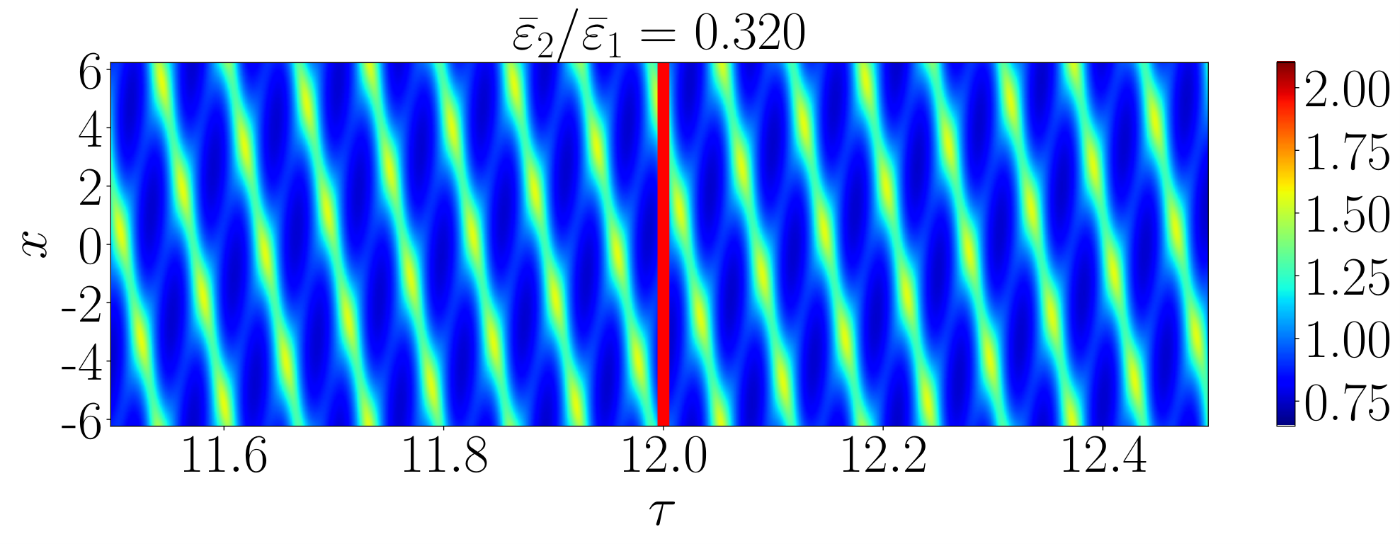
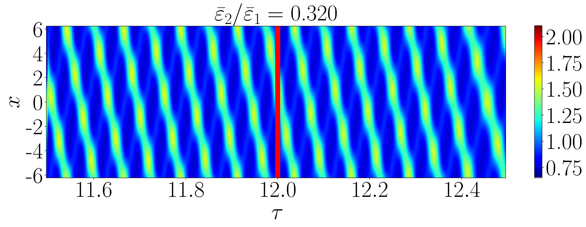
The important dynamical characteristic of the autoresonance is that when starting from zero, the chirped-driven system is captured into resonance only if the driving amplitudes exceed a certain threshold (Barth and Friedland 2007). Thus, if we increase the amplitudes of the drives, the autoresonant excitation of the quasicrystals occurs abruptly, resembling a phase transition.
The thresholds can be analyzed by reducing the problem to the motion of pseudoparticles in an anharmonic slowly varying potential well, similar to the way it was done in Ref. (Fajans and Frièdland 2001) for the single phase weakly nonlinear theory. However, unlike the threshold for the autoresonance of a single phase ion acoustic wave (see Ref. (Friedland and Shagalov 2014)), the general analytical result for the double autoresonance thresholds is difficult to obtain and the thresholds are complicated functions of , , , , . Nonetheless, it is possible to find the thresholds numerically. As an example let us use the same parameters as in Figs. 1(a), 2, 3, and 4, fix the value of , and solve numerically both the fully and weakly nonlinear equations while sweeping through values of . The results of these simulations are presented in Figs. 7 and 8. Figure 7 shows a colormap of the electron density obtained by solving the fully nonlinear equations (1)–(3) for various values of : just above the threshold at (top subplot), just below the threshold at (middle subplot), and below the threshold at (bottom subplot), while Fig. 8 shows a colormap of the electron density obtained by solving the weakly nonlinear equations (38)–(41) for various values of : just above the threshold (, top subplot), just below the threshold (, middle subplot), and below the threshold (, bottom subplot). We can see from these figures that the crystallization is indeed an abrupt phenomenon akin to a phase transition. For the fully nonlinear simulations the threshold lies between and , while for the weakly nonlinear simulations the threshold lies between and . Such a good agreement for the value of the threshold is another proof that our weakly nonlinear theory is applicable. To better illustrate the threshold nature of the double autoresonance we also produced an animation showing the crystallization of a single phase structure into a two-phase structure around the threshold as we sweep from to . The animation is available in the Supplemental Material (ani).
The necessity of the phase locking for the autoresonance is demonstrated in Fig. 9, which shows the effective actions and the phase mismatches as functions of slow time just below the threshold (, left side) and just above the threshold (, right side). One can clearly see that just below the threshold the second action does not enter the autoresonant regime and the growth of the amplitude saturates, while the phase mismatch increases with time signifying the absence of phase locking. In contrast, just above the threshold both phases are locked and the amplitudes increase in time similar to the case shown in Fig. 4.
V Conclusions
We have demonstrated by means of nonlinear numerical simulations that it is possible to create quasicrystalline spatiotemporal structures in plasma by exciting large amplitude two-phase ion acoustic waves nonlinearly phased locked into the corresponding small amplitude traveling wave drives with chirped frequencies. We have used the Lagrangian formulation and Whitham’s averaged variational method to derive analytical results describing the weakly nonlinear evolution of the system. We have applied the weakly nonlinear analytical theory to determine the parameters necessary for the successful excitation and control of multiphase waves. The nonlinearly excited quasicrystalline structures remain even after we turn off the drive. Thus, the space-time quasicrystalline structure in plasma can be excited and then used independently for the purpose of plasma photonics experiments. While our warm fluid model does not have dissipation or noise due to collisions or Landau damping, for example, and, generally speaking, its long-time stability must be addressed by kinetic or particle-in-cell (PIC) simulations, it is apparent that, depending on the time scales of the problem, this structure can be considered as at least a dissipative space-time crystal. We also note that we do not address in this paper whether the driven space-time crystal is a “true” time crystal in the sense of spontaneous symmetry breaking as proposed in Refs. (Wilczek 2012; Shapere and Wilczek 2012); for more discussion regarding this see Refs. (Yao et al. 2020; Sacha 2020; Else et al. 2020).
It is expected that, using our technique, similar structures can be driven in other systems, for example dust acoustic waves in complex plasmas (Rao et al. 1990). We expect that multiphase solutions when the number of drives exceeds two are also possible; however, it will be harder to analyze such a system analytically. Finally, we point out that beyond any practical application as a plasma photonic (or accelerating) structure, the possibility of exciting multiphase solutions for in general non-integrable warm ion acoustic waves system is in itself an important fundamental result in the field of nonlinear dynamics. These techniques developed for the excitation of large amplitude ion acoustic waves may be applied to other partial differential equation systems that can support multiphase nonlinear waves.
Acknowledgments
This work was supported by NSF-BSF Grant No. 1803874 and US-Israel Binational Science Foundation Grant No. 2020233.
Appendix A The averaged Lagrangian density
The averaged Lagrangian density
| (45) |
is equal to the sum of the following terms:
| (46) |
| (47) |
| (48) |
| (49) |
| (50) |
| (51) |
| (52) |
| (53) |
| (54) |
Appendix B The variations and the amplitudes
In this Appendix we calculate the variations of the averaged Lagrangian with respect to the various amplitudes and express all the second-order amplitudes , , , , , , , , , , , through the first-order amplitudes and .
To express the second-order amplitudes through and let us first calculate the variations of the averaged Lagrangian density with respect to the second-order amplitudes:
| (55) |
| (56) |
| (57) |
| (58) |
| (59) |
| (60) |
| (61) |
| (62) |
| (63) |
| (64) |
| (65) |
| (66) |
| (67) |
From Eq. (55) we obtain
| (68) |
| (69) |
| (70) |
| (71) |
| (72) |
| (73) |
| (74) |
| (75) |
| (76) |
| (77) |
| (78) |
| (79) |
| (80) |
| (81) |
| (82) |
| (83) |
| (84) |
| (85) |
| (86) |
| (87) |
| (88) |
| (89) |
| (90) |
| (91) |
| (92) |
Note that in the limiting case of cold ions and with two identical counter propagating traveling waves (i.e., a standing wave with , , ) the above amplitudes coincide with the amplitudes derived in Ref. (Friedland et al. 2019), as expected. In particular, the amplitudes , , , , , , , , from Ref. (Friedland et al. 2019) are related to the amplitudes in this paper as follows:
| (93) | |||
| (94) | |||
| (95) |
To derive weakly nonlinear equations we also need to calculate the variations of with respect to the first-order amplitudes:
| (96) |
| (97) |
| (98) |
| (99) |
| (100) |
| (101) |
Appendix C Functions and
Function is defined through
| (102) |
or, equivalently due to symmetry, through
| (103) |
while is defined through
| (104) |
References
- Joannopoulos (2008) J. Joannopoulos, Photonic Crystals: Molding the Flow of Light (Second Edition) (Princeton University Press, Princeton, 2008).
- Ho et al. (1990) K. M. Ho, C. T. Chan, and C. M. Soukoulis, Phys. Rev. Lett. 65, 3152 (1990).
- John (1987) S. John, Phys. Rev. Lett. 58, 2486 (1987).
- Yablonovitch (1987) E. Yablonovitch, Phys. Rev. Lett. 58, 2059 (1987).
- Hojo and Mase (2004) H. Hojo and A. Mase, J. Plasma Fusion Res. 80, 89 (2004).
- Hojo and Mase (2009) H. Hojo and A. Mase, J. Plasma Fusion Res. 8 (2009).
- Solaimani (2020) M. Solaimani, Results Phys. 16, 102843 (2020).
- Qi et al. (2010) L. Qi, Z. Yang, F. Lan, X. Gao, and Z. Shi, Phys. Plasmas 17, 042501 (2010).
- Rahmani and Rezaee (2019) Z. Rahmani and N. Rezaee, Optik 184, 134 (2019).
- Li et al. (2009) W. Li, Y. Zhao, R. Cui, and H. Zhang, Font. Optoelectron. China 2, 103 (2009).
- Zhang and Ouyang (2014) L. Zhang and J.-T. Ouyang, Phys. Plasmas 21, 103514 (2014).
- Sakai et al. (2005) O. Sakai, T. Sakaguchi, Y. Ito, and K. Tachibana, Plasma Phys. Control. Fusion 47, B617 (2005).
- Sakai and Tachibana (2012) O. Sakai and K. Tachibana, Plasma Sources Sci. Technol. 21, 013001 (2012).
- Qi et al. (2015) L. Qi, C. Li, G. Fang, and X. Gao, Plasma Sci. Technol. 17, 4 (2015).
- Zhang et al. (2013) H.-F. Zhang, S.-B. Liu, X.-K. Kong, Chen-Chen, and B.-R. Bian, Phys. Plasmas 20, 042110 (2013).
- Zhang et al. (2013) H.-F. Zhang, S.-B. Liu, and X.-K. Kong, J. Light. Technol. 31, 1694 (2013).
- Suzuki et al. (2014) K. Suzuki, K. Kitano, K. Ishizaki, and S. Noda, Opt. Express 22, 17099 (2014).
- Liang et al. (2021) Y. Liang, Z. Liu, L. Lin, J. Peng, R. Liu, and Q. Lin, Appl. Opt. 60, 2510 (2021).
- Wang and Cappelli (2016) B. Wang and M. A. Cappelli, Appl. Phys. Lett. 108, 161101 (2016).
- Levine and Steinhardt (1984) D. Levine and P. J. Steinhardt, Phys. Rev. Lett. 53, 2477 (1984).
- Dyachenko et al. (2012) P. N. Dyachenko, V. S. Pavelyev, and V. A. Soifer, Opt. Lett. 37, 2178 (2012).
- Poddubny and Ivchenko (2010) A. Poddubny and E. Ivchenko, Physica E 42, 1871 (2010).
- Lifshitz et al. (2005) R. Lifshitz, A. Arie, and A. Bahabad, Phys. Rev. Lett. 95, 133901 (2005).
- Vardeny et al. (2013) Z. V. Vardeny, A. Nahata, and A. Agrawal, Nat. Photonics 7, 177 (2013).
- Bahabad et al. (2008) A. Bahabad, A. Ganany-Padowicz, and A. Arie, Opt. Lett. 33, 1386 (2008).
- Freedman et al. (2006) B. Freedman, G. Bartal, M. Segev, R. Lifshitz, D. N. Christodoulides, and J. W. Fleischer, Nature 440, 1166 (2006).
- Neve-Oz et al. (2010) Y. Neve-Oz, T. Pollok, S. Burger, M. Golosovsky, and D. Davidov, J. Appl. Phys. 107, 063105 (2010).
- Chan et al. (1998) Y. S. Chan, C. T. Chan, and Z. Y. Liu, Phys. Rev. Lett. 80, 956 (1998).
- Lustig et al. (2018) E. Lustig, Y. Sharabi, and M. Segev, Optica 5, 1390 (2018).
- Zurita-Sánchez et al. (2009) J. R. Zurita-Sánchez, P. Halevi, and J. C. Cervantes-González, Phys. Rev. A 79, 053821 (2009).
- Zurita-Sánchez et al. (2012) J. R. Zurita-Sánchez, J. H. Abundis-Patiño, and P. Halevi, Opt. Express 20, 5586 (2012).
- Zurita-Sánchez and Halevi (2010) J. R. Zurita-Sánchez and P. Halevi, Phys. Rev. A 81, 053834 (2010).
- Salem and Caloz (2015) M. A. Salem and C. Caloz, in 2015 International Conference on Electromagnetics in Advanced Applications (ICEAA) (2015) pp. 490–493.
- Martínez-Romero and Halevi (2018) J. S. Martínez-Romero and P. Halevi, Phys. Rev. A 98, 053852 (2018).
- Sacha (2020) K. Sacha, Photonic time crystals, in Time Crystals (Springer International Publishing, Cham, 2020) pp. 251–265.
- Wang et al. (2018) N. Wang, Z.-Q. Zhang, and C. T. Chan, Phys. Rev. B 98, 085142 (2018).
- Park and Min (2021) J. Park and B. Min, Opt. Lett. 46, 484 (2021).
- Biancalana et al. (2007) F. Biancalana, A. Amann, A. V. Uskov, and E. P. O’Reilly, Phys. Rev. E 75, 046607 (2007).
- Biancalana et al. (2008) F. Biancalana, A. Amann, and E. P. O’Reilly, Phys. Rev. A 77, 011801 (2008).
- Zeng et al. (2017) L. Zeng, J. Xu, C. Wang, J. Zhang, Y. Zhao, J. Zeng, and R. Song, Sci. Rep. 7, 17165 (2017).
- Caloz and Deck-Léger (2020a) C. Caloz and Z.-L. Deck-Léger, IEEE Trans. Antennas Propag. 68, 1569 (2020a).
- Caloz and Deck-Léger (2020b) C. Caloz and Z.-L. Deck-Léger, IEEE Trans. Antennas Propag. 68, 1583 (2020b).
- Sharabi et al. (2020) Y. Sharabi, E. Lustig, A. Dikopoltsev, Y. Lumer, and M. Segev, in 2020 Conference on Lasers and Electro-Optics (CLEO) (2020) pp. 1–2.
- Milchberg (2019) H. Milchberg, Physics Today 72, 70 (2019).
- Durfee and Milchberg (1993) C. G. Durfee and H. M. Milchberg, Phys. Rev. Lett. 71, 2409 (1993).
- Malkin et al. (1999) V. M. Malkin, G. Shvets, and N. J. Fisch, Phys. Rev. Lett. 82, 4448 (1999).
- Thaury et al. (2007) C. Thaury, F. Quéré, J. P. Geindre, A. Levy, T. Ceccotti, P. Monot, M. Bougeard, F. Réau, P. d’Oliveira, P. Audebert, R. Marjoribanks, and P. Martin, Nat. Phys. 3, 424 (2007).
- Doumy et al. (2004) G. Doumy, F. Quéré, O. Gobert, M. Perdrix, P. Martin, P. Audebert, J. C. Gauthier, J.-P. Geindre, and T. Wittmann, Phys. Rev. E 69, 026402 (2004).
- Dromey et al. (2004) B. Dromey, S. Kar, M. Zepf, and P. Foster, Rev. Sci. Instrum. 75, 645 (2004).
- Kapteyn et al. (1991) H. C. Kapteyn, M. M. Murnane, A. Szoke, and R. W. Falcone, Opt. Lett. 16, 490 (1991).
- Michel et al. (2009a) P. Michel, L. Divol, E. A. Williams, S. Weber, C. A. Thomas, D. A. Callahan, S. W. Haan, J. D. Salmonson, S. Dixit, D. E. Hinkel, M. J. Edwards, B. J. MacGowan, J. D. Lindl, S. H. Glenzer, and L. J. Suter, Phys. Rev. Lett. 102, 025004 (2009a).
- Michel et al. (2009b) P. Michel, L. Divol, E. A. Williams, C. A. Thomas, D. A. Callahan, S. Weber, S. W. Haan, J. D. Salmonson, N. B. Meezan, O. L. Landen, S. Dixit, D. E. Hinkel, M. J. Edwards, B. J. MacGowan, J. D. Lindl, S. H. Glenzer, and L. J. Suter, Phys. Plasmas 16, 042702 (2009b).
- Lehmann and Spatschek (2016) G. Lehmann and K. H. Spatschek, Phys. Rev. Lett. 116, 225002 (2016).
- Lehmann and Spatschek (2017) G. Lehmann and K. H. Spatschek, Phys. Plasmas 24, 056701 (2017).
- Lehmann and Spatschek (2018) G. Lehmann and K. H. Spatschek, Phys. Rev. E 97, 063201 (2018).
- Michel et al. (2014) P. Michel, L. Divol, D. Turnbull, and J. D. Moody, Phys. Rev. Lett. 113, 205001 (2014).
- Michel et al. (2020) P. Michel, E. Kur, M. Lazarow, T. Chapman, L. Divol, and J. S. Wurtele, Phys. Rev. X 10, 021039 (2020).
- Kur et al. (2021) E. Kur, M. Lazarow, J. S. Wurtele, and P. Michel, Opt. Express 29, 1162 (2021).
- Friedland and Shagalov (2020) L. Friedland and A. G. Shagalov, J. Plasma Phys. 86, 825860301 (2020).
- Friedland et al. (2019) L. Friedland, G. Marcus, J. S. Wurtele, and P. Michel, Phys. Plasmas 26, 092109 (2019).
- Scott (1999) A. Scott, Nonlinear Science: Emergence and Dynamics of Coherent Structures (Oxford University Press, 1999).
- Novikov et al. (1984) S. Novikov, S. V. Manakov, L. P. Pitaevskii, and V. E. Zakharov, Theory of Solitons: The Inverse Scattering Method (Consultants Bureau, New York, 1984).
- Friedland and Shagalov (2003) L. Friedland and A. G. Shagalov, Phys. Rev. Lett. 90, 074101 (2003).
- Friedland and Shagalov (2005) L. Friedland and A. G. Shagalov, Phys. Rev. E 71, 036206 (2005).
- Shagalov and Friedland (2009) A. Shagalov and L. Friedland, Physica D 238, 1561 (2009).
- Khasin and Friedland (2003) M. Khasin and L. Friedland, Phys. Rev. E 68, 066214 (2003).
- Friedland and Shagalov (2014) L. Friedland and A. G. Shagalov, Phys. Rev. E 89, 053103 (2014).
- Friedland and Shagalov (2017) L. Friedland and A. G. Shagalov, Phys. Plasmas 24, 082106 (2017).
- Washimi and Taniuti (1966) H. Washimi and T. Taniuti, Phys. Rev. Lett. 17, 996 (1966).
- Whitham (1999) G. B. Whitham, Linear and Nonlinear Waves (Wiley, New York, 1999).
- Kakad et al. (2017) B. Kakad, A. Kakad, and Y. Omura, Phys. Plasmas 24, 102122 (2017).
- Riconda et al. (2005) C. Riconda, A. Heron, D. Pesme, S. Hüller, V. T. Tikhonchuk, and F. Detering, Phys. Rev. Lett. 94, 055003 (2005).
- Barth and Friedland (2007) I. Barth and L. Friedland, Phys. Rev. E 76, 016211 (2007).
- Fajans and Frièdland (2001) J. Fajans and L. Friedland, Am. J. Phys. 69, 1096 (2001).
- (75) See Supplemental Material at https://doi.org/10.6084/m9.figshare.17912333.v1 for an animation showing the crystallization of a single phase structure into a two-phase structure around the threshold.
- Wilczek (2012) F. Wilczek, Phys. Rev. Lett. 109, 160401 (2012).
- Shapere and Wilczek (2012) A. Shapere and F. Wilczek, Phys. Rev. Lett. 109, 160402 (2012).
- Yao et al. (2020) N. Y. Yao, C. Nayak, L. Balents, and M. P. Zaletel, Nat. Phys. 16, 438 (2020).
- Else et al. (2020) D. V. Else, C. Monroe, C. Nayak, and N. Y. Yao, Annu. Rev. Condens. Matter Phys. 11, 467 (2020).
- Rao et al. (1990) N. Rao, P. Shukla, and M. Yu, Planet. Space Sci. 38, 543 (1990).