Formal models of Memory Formal Models of Memory \rightheaderFormal models of Memory \noteIn press, In F. G. Ashby, H. Colonius, & E. Dzhafarov (Eds.), The new handbook of mathematical psychology, Volume 3. Cambridge University Press.
Formal models of memory based on temporally-varying representations
Abstract
The idea that memory behavior relies on a gradually-changing internal state has a long history in mathematical psychology. This chapter traces this line of thought from statistical learning theory in the 1950s, through distributed memory models in the latter part of the 20th century and early part of the 21st century through to modern models based on a scale-invariant temporal history. We discuss the neural phenomena consistent with this form of representation and sketch the kinds of cognitive models that can be constructed using it and connections with formal models of various memory tasks.
Human babies, while adorable, are remarkably incompetent. They know essentially no facts about the world and are unable to perform any but the simplest motor actions, and perform very poorly on behavioral assays of memory. Memory researchers evaluate memory in adults with a variety of behavioral paradigms, such as cued recall, in which the participant is given a series of pairs, e.g., absence-hollow, pupil-river, campaign-helmet. The participants’ task is to produce the correct associate when given a cue word. For instance, after being probed with pupil the correct response is river. After being presented with a list of words for a cued recall test, a human baby is more likely to emit curdled milk than a correct response. Over the course of a lifetime, normally-developing humans learn many facts about their world, acquire complicated motor skills and can bring to mind vivid recollections of many events from their lives. Because all of these abilities must be learned, they can be understood as forms of memory.
Viewed in this light, the task of a memory theorist seems daunting. How can one possibly construct a theory that can make sense of the ability to recall that Paris is the capitol of France, the ability to ride a bike without falling over, and the ability to vividly remember a birthday party well enough to bring a smile to one’s face after decades? The strategy taken by cognitive neuroscientists in the latter part of the 20th century (and continuing to the present day) is to carve up the set of abilities and skills that differentiate a baby from an adult into different “kinds” of memory, each associated with distinct parts of the brain. For instance, many memory researchers would say that retrieving facts about the world depends on semantic memory, being able to ride a bicycle is a consequence of implicit memory and vivid recollection of specific events from ones life relies on episodic memory. This strategy of dividing learning and memory phenomena into different “kinds of memory” has been extremely productive. However, throughout the history of psychology, there has been an urge towards developing unified theories of learning and memory.
0.1 Associations in the mind and brain
Radical behaviorists (most famously B. F. Skinner) attempted to understand the rich repertoire of memory phenomena as special cases of stimulus-response associations. Pavlov’s dogs learned to associate the sound of a bell with the delivery of food, so that the sound of the bell by itself leads to an overt response (salivation). Experimentalists learned that animals (in particular rats and pigeons) can be trained to perform complex sequences of behaviors in response to appropriate training experiences. According to behaviorists’ conception of learning, even complex behaviors could be described as complex chains of associations.
Mathematical psychologists have developed formal models of association to provide quantitative models of behavior in a variety of experimental paradigms. Early work focused on animal conditioning experiments. In this case the behavioral measure is typically a scalar value that describes the probability or magnitude of a conditioned response; for instance, the amount of saliva produced by Pavlov’s dog (or, more typically, the proportion of time the animal spends freezing in a fear conditioning experiment). But later work also applied similar ideas to memory experiments with humans using lists of words as stimuli. In the cued recall task described above, it is straightforward to write down a model that constructs simple associations between neural representations of the words (e.g., associate absence to hollow) such that probing the memory with the stimulus absence causes a pattern like hollow to be produced as an output. These models can produce many distinct responses in responses to many different cues.
Associations can be understood neurally as a consequence of changes in the connection strength between neurons. The mammalian brain contains a great number of specialized cells called neurons. Neurons are known to communicate information between one another by means of their electrical activity. The connections between individual neurons are referred to as synapses. The strength of synapses can be modified by experience. These facts are sufficient to write down a very crude neural model of Pavlovian conditioning. If one identifies the set of neurons that changes its firing in response to the sound of the bell, and the set of neurons responsible for salivation, one could in principle understand the association learned by Pavlov’s dog as an increase in the strength of the synapses connecting the “bell” neurons to the “drool” neurons. These assumptions can be formalized in tractable mathematical models that are (at least) neurally reasonable. Extending this idea to models of more elaborate tasks, such as human cued recall requires mapping each of the stimuli that will be part of the experiment – i.e., each of the words in the list – to a pattern of activation over neurons. This is typically done by mapping each word to a vector in a space of neurons. In this case, the synapses between the neurons can be understood as a matrix. With appropriate assumptions, many results can be derived and a particular set of assumptions can be compared to behavior.
0.2 Cognitive models of memory
The basic theoretical stance of behaviorism is that we should construct psychological theory without reference to the internal state of the organism. This approach is difficult to reconcile with many human laboratory memory tasks. For instance, a radical behaviorist model of the free recall task is untenable. In free recall, participants are presented with a sequential experiece (e.g., a list of words) and later asked to verbally report their memory for the experience. What is the “cue” in free recall? Participants can report many different experiences and can report on different aspects of their experience. It is difficult to make sense of these phenomena without simply assuming that the participant has some internal experience of their memory that they then describe.
Cognitive models make a hypothesis about the internal state of the organism and use that hypothesis to predict behavior. Radical behaviorists explicitly eschewed any reference to the internal experience of the behaving organism under the belief that such theorizing was underconstrained and can not lead to a satisfactory scientific theory. However, advances in modern neuroscience have made this concern largely obsolete. In principle, cognitive models can simultaneously describe the observable behavior of an organism and neural observables from the brain during performance of that behavior. In this way, cognitive models can be constrained by comparison to activity of neurons in the brain.
A broad class of cognitive models proceed by building simple associations between stimuli mediated by a hypothesized internal state. For instance, short-term memory models hypothesize the existence of a short-term store that holds information about recently presented stimuli. According to one influential approach, associations between stimuli can only be formed among stimuli that are simultaneously active in the short-term store Atkinson & Shiffrin (1968); Raaijmakers & Shiffrin (1980). Another widely-used approach assumes the existence of a “temporal context” that mediates associations between items Sederberg et al. (2008); Polyn et al. (2009). Temporal context models assume that the brain maintains a representation at each moment of the recent past. This temporal context changes gradually. When a person remembers a specific instance from their past (like vividly remembering a particular event such as a birthday), this cognitive event is accompanied by a recovery of temporal context. These models make specific neural predictions. Short-term memory models and temporal context models predict that it ought to be possible to examine the activity of neurons in the brain (using electrodes or non-invasive methods such as EEG or fMRI) and decode the content of recent experiences. Cognitive models of this class are introduced in Section 2.
0.3 Beyond associations: Representing temporal relationships in the mind and brain
Although associations have been an extremely productive idea in the mathematical psychology of memory, there is no question that simple associations as understood by behaviorists are insufficient to describe the richness of human memory. Associations that can be described by a scalar value are extremely limited. If the association between stimulus x and stimulus y is some specific number, say 2.38, and the association between x and z is 0.35, we can say that the x y association is stronger than the x z association. Operationally, if we probe memory with x, memory returns “more” y than z. However, human memory can learn and express many different kinds of relationships. For instance, x might be two meters to the East of y, or x might be a member of the category z, or y and z might be married to one another. In order to express these kinds of relationships, a richer formalism is required.
The mammalian brain contains neurons that can express metric relationships between stimuli. For instance, consider neurons referred to as “time cells” in the rodent hippocampus during performance of a behavioral task Eichenbaum (2017). After presentation of a stimulus, e.g., ringing a bell, these time cells fire in a sequence such that each neuron fires for a circumscribed period of time (e.g., Figure 6). Because the sequence is reliable across different presentations of the same stimulus, it is possible to look at which time cell is firing and decode how far in the past the triggering stimulus was experienced. As we will see, the information about the time in the past at which the bell was presented written across this population of neurons can be used to learn temporal relationships between the presentation of the bell and other stimuli. This class of models has been used to develop cognitive models of relatively complex behavioral tasks and at the same time the properties of time cells can be evaluated against experiments recording from populations of neurons in mammals. To the extent that this hypothesis is consistent with both behavioral and neurophysiological data, it makes sense to take the equations seriously. As we will see, the formalism is quite rich, providing an opportunity to do meaningful theoretical work on physical models of memory.
0.4 A brief history of mathematical models of memory
This chapter covers a tiny proportion of the work in mathematical models of human memory. To provide at least pointers to the topics that are missing, and to properly contextualize the topics that are covered, this subsection provides a very concise history of mathematical models of memory.
Descriptive quantitative models of behavior date back to the very beginning of modern memory research. Ebbinghaus (1885/1913) conducted early empirical studies of human memory, testing himself on serial recall of nonsense syllables. Ebbinghaus (1885/1913) included quantitative descriptions of many of the phenomena he studied. For instance, Ebbinghaus introduced the power law of forgetting to describe his findings relating the persistence of memory to the passage of time. In the early part of the 20th century, radical behaviorism led many researchers to focus on simple stimulus-response associations. Quantitative models of these data attempted to describe observable phenomena with as few assumptions as possible. Hull (1939) provides an excellent example of the spirit of this work, fitting equations to observed empirical relationships.
The 1950s saw the first process models of memory. Process models, in contrast to descriptive models, make hypotheses about internal mechanisms that cause observable behavior. Stimulus sampling theory Estes (1950); Bush & Mosteller (1951), provides an early example of such a process model. Stimulus sampling theory introduced a number of ideas that are still extremely influential today (see section 1).
The 1960s and 1970s saw memory research divide into a set of subfields as the cognitive revolution dramatically changed the kinds of theories that were acceptable in psychology. There were two major developments in mathematical models of memory during this era that had long-lasting effects over the next several decades. First, building on a long tradition of mathematical models of conditioning, the Rescorla-Wagner model (Rescorla & Wagner (1972), see Chapter 5) successfully accounted for essentially everything that was known about classical conditioning up to that time. The Rescorla-Wagner model is built on a really simple idea – that change in an association between a cue and a response depends on how well the outcome is predicted. Second, the 1960s saw the development of the first models of short-term memory building on early ideas from Miller (1956). The two-store memory model of Atkinson & Shiffrin (1968) provided a conceptually simple description of an immense amount of data (see Section 2). This was also perhaps the first influential mathematical model of memory to make use of computer simulations to test its predictions. These two very different models spawned entire fields of research in psychology and neuroscience that continue to this day.
The Rescorla-Wagner model led directly to reinforcement learning Sutton & Barto (1981). Reinforcement learning has been extremely influential in neuroscience, where the connection between these models and the dopamine system in the brain Schultz et al. (1997) has spawned an immense amount of work that continues to the present (e.g., see Ashby, Crossley, Inglis, this volume). Reinforcement learning has also been extremely influential in artificial intelligence research, including very high profile papers building models to achieve human-level performance in video games and the game of go Mnih et al. (2015); Silver et al. (2016).
The Atkinson & Shiffrin (1968) model also led to a great deal of work in psychology and neuroscience. The model coincided with the discovery of patients with brain damage that showed problems with short-term memory but not long-term memory, and vice versa. Baddeley & Hitch (1977) further subdivided short-term store and mapped these components onto distinct brain circuits. This kind of model – with many components that map onto different parts of the brain – was well-suited for posing the kinds of questions that could be answered with early cognitive neuroimaging techniques such as PET and univariate fMRI. Mathematical models of short-term memory continue to be influential in contemporary cognitive neuroscience (see Trutti et al. (2021) for a recent review).
In the 1980s and 1990s, a great deal of attention was focused on a class of mathematical models of memory that were collectively known as distributed memory models. These models focused on human memory experiments, primarily experiments that would be understood today as episodic memory tasks. Models that fall into this class include TODAM Murdock (1982), CHARM Metcalfe (1985), SAM Gillund & Shiffrin (1984), MINERVA-2 D. Hintzman (1987), the matrix model Humphreys et al. (1989), and REM Shiffrin & Steyvers (1997). Although these models differed in many details, there were some common assumptions. First, they represented studied items as a distributed set of features, building on early work by Anderson (1972); Anderson (1973). Section 1 also adopts this convention. Second, the distributed memory models were all associative. It was implicit that short-term memory controlled which items and associations were stored in memory. An important conceptual contribution of these models was the introduction of quantitative models for context (Murdock (1997), see especially) that we build on in Section 2. The temporal context models discussed in section 2 grew out of this tradition.
The early distributed memory models did not make a connection to neuroscience. In contrast, connectionist models of memory (see Hasselmo & McClelland (1999) for a review of early work) paid close attention to neuroscience. For the most part, these models did not focus on detailed behavioral data from human memory experiments (Hasselmo & Wyble (1997); Norman & O’Reilly (2003), but see). Rather, these models focused more on problems, such as amnesia and sleep, that had a clear connection to neural processes. For instance, in one very influential paper McClelland et al. (1995) postulated that behavioral patterns observed in amnesia patients – for instance the ability to remember events from early in ones life but not the ability to remember more recent events – were attributable to separate memory stores that learned associations with different statistics. Connectionist memory models were developed in parallel with advances in artificial neural networks that are fundamental to contemporary AI.
One very important development in the early part of the 20th century was that models of conditioning made contact with models of timing behavior. Scalar expectancy theory Gibbon (1977) provided an excellent model of behavioral experiments where animals had to use their sense of time to receive reward (Killeen & Fetterman (1988), see also). Gallistel & Gibbon (2000) constructed a mathematical model out of scalar expectancy theory that described a range of findings from conditioning experiments. The hypothesis was that behavioral associations fundamentally result from learning about the temporal relationships between the stimulus and response. Balsam & Gallistel (2009) provide an elegant overview of this idea. Notably, because timing behavior has the same properties over a range of time scales, models of conditioning built on this assumption can naturally accommodate scale-invariance in memory, which is discussed further in section 2.6.
Section 3 draws on work over the last decade or so that synthesizes aspects of many of these approaches. The scale-invariant temporal history was originally proposed to address limitations in temporal context models Shankar & Howard (2010). As such it is continuous with the distributed memory models and can be used to build models of similar tasks. At the same time, because neuroscientific considerations place such strong constraints on these models, it is similar in spirit to the connectionist models of memory. Finally, because memory traces are formed using a population that contains information about the time at which events took place, this approach is closely related to (and in actual fact was very much inspired by) work pursuing a close relationship between timing and conditioning.
1 “Simple” associations in the mind and brain
In this section we will introduce a formalism to describe mathematical models based on simple associations. We will suppose that learning consists of forming and accessing associations between a set of “items.” These items can correspond to words in a cued recall experiment, in which we attempt to describe the association between two words (e.g., absence–hollow above). Or we could use the same formalism to describe the association between a tone that serves as a conditioned stimulus and an unconditioned response, such as salivation in the case of Pavlov’s dog.
Distributed memory models (DMM) assume that each item is described by a vector over some high dimensional space. We will write vectors as lower-case bold letters, , where is some “large” integer. We can envision the vector as a list of numbers that describes the activity over a large population of neurons. If a particular item represents a word we might understand as the “pattern of activity” over a population of neurons that are caused by presentation of that word. A different word would produce a different pattern of activity. If a particular item corresponds to a response, such as salivation, we might understand as the pattern of activity in a particular population that is necessary for salivation rather than some other response (such as freezing).
1.1 Hebbian learning
As an illustration of the distributed-memory model approach, let us consider a simple model of cued recall. We map all of the words that could possibly be presented in an experiment onto a set of vectors within the same space. We assume further that the overwhelming majority of entries are zero and the remainder are some small positive number and that the number of entries is large. Suppose that we randomly choose vectors corresponding to two different words and . We can take the inner product between any two vectors as a measure of their “similarity.” With these assumptions, the inner product of a vector with itself, or will tend to be much greater than the inner product between different words , because the entries of these are not perfectly correlated. We might even suppose that related words (e.g., couch and sofa) correspond to vectors that are more similar to one another than unrelated words (e.g., couch and rutabaga). To keep the arithmetic simple, let us suppose that we have chosen the entries in the vectors to ensure that the expected value of is 1 if and close to zero otherwise.
Let us flesh this model out sufficiently to model a simple cued recall experiment. Let us describe a list of word pairs by denoting the cue of the pair presented at time with a vector and the response member of the pair with a vector . So, if we had a list of two pairs, absence–hollow and pupil–river, we would refer to the vector corresponding to absence as , the vector corresponding to hollow as , the vector correspoding to pupil as and river as .
Now, we can model associations between the words as an outer product matrix between the vectors corresponding to the cue and response of each pair. Let us assume that the matrix is initialized as an matrix of zeros before the list. Then as each item is presented, is updated as:
| (1) |
so that after learning the entire list,
| (2) |
where the sum is over all of the pairs presented in the experiment.
To understand the role of the outer product, let us imagine we have a one-pair list so that (Fig. 1). Any particular entry gives the product of the activity in “neuron ” in pattern and “neuron ” in pattern . The product is non-zero if both and are non-zero. The anatomical structure that connects the axon of one neuron to the dendrite of another is referred to as a synapse. These connections can be strengthened or weakened based on the activity of the pre- and post-synaptic neurons through a variety of molecular processes. Hebbian learning (originally proposed by Donald Hebb in 1948) is a learning rule in which synapses are strengthened if both the pre- and post-synaptic neurons are active at the same time (see Ashby et al., this volume, for more details). Informally, Hebbian learning is often summarized by the slogan “neurons that fire together, wire together.” Hebbian learning has been demonstrated experimentally in a number of brain regions and a number of species.
To understand why this is referred to as an association, let us probe with a probe word, which we denote as . Then we find that . That is, probing with a probe vector returns weighted by the similarity between the probe vector and the studied cue vector. If the probe vector is the same as the studied cue , the output is multiplied by a large number. If is not the same as , the output is mutiplied by a small number. Returning to the situation where there are many pairs in the list, we find, exploiting the linearity of matrix addition and commutativity of multiplication by a scalar,
| (3) | |||||
| (4) |
That is, after probing memory with a specific word , the output is the vector sum of the response words weighted by the similarity of the probe word to the cue that was paired with that response. Because the similarity of the probe words to themselves is much greater than between different words, this sum gives a large number for the appropriate response and much smaller numers for the other possible responses. If one probes with , the output is “mostly” ; if one probes with , the output is mostly . By adding assumptions that map the output of the associative memory onto a probability of successfully recalling the appropriate response, one can construct relatively elaborate models of behavior.
If each component of and can be thought of as a neuron, then each entry in can be understood as a synapse. The entire matrix can thus be understood as the set of synapses connecting the two populations. The outer product learning rule in Eq. 1 can thus be understood as a simple hypothesis for how populations of neurons can store information via Hebbian learning. Although this is undoubtedly a grotesque oversimplification of what happens in the brain, this framework is sufficiently simple that one can write out tractable models of behavioral experiments.
To actually compare this model to behavioral data, it’s necessary to specify some means to map the strength of the association onto behavioral observables, for instance probability of recall. Having said that, this simple Hebbian mechanism responds appropriately to many experimental manipulations in a sensible way. For instance, suppose that some pairs in the list are repeated. Adding additional terms with the same vectors to Eq. 2 results in a stronger association between those items (this follows from linearity).11 1 One can easily construct a similar argument for the effect of increasing the study time for some of the pairs in the list. Similarly, one can compare recall of a particular pair in lists of various lengths. Examining Eq. 4, we see that the effect of including additional pairs is to add noise to the output of memory. That is, after probing with , the output of memory is times a big number plus all of the other items in the list weighted by small numbers. As one adds pairs to the list, this second component grows more important, acting like background noise for retrieval of the target response. Similarly, one could imagine that attention fluctuates from moment-to-moment and model that by multiplying Eq. 1 by a factor that estimates the current amount of attention. Distributed memory models pursued questions along these lines and carefully compared the results to behavioral experiments.
1.2 Forgetting
The Hebbian outer product model sketched above has several problems, many of which are addressed by subsequent work described in the remainder of this chapter. Here we discuss ways to enable the model to forget. We discuss two approaches to forgetting. Perhaps the most obvious way to implement forgetting is to allow the weights to decrease in amplitude. A less obvious way to implement forgetting is to assume that the cue itself is not constant over time. That is, although an experimenter may take care to present the word absence several times in the same font, in the same location of the screen, for precisely the same duration of time, this does not ensure that this stimulus activates the same set of neurons in the brain on each presentation. There are many other possible approaches to forgetting and different mechanisms may contribute differentially to forgetting in different experimental paradigms. This chapter focuses on these two mechanisms for forgetting because they lend themselves to concise mathematical descriptions and are conceptually distinct from one another.
1.2.1 Forgetting via changes in the weight matrix
One simple way to augment Eq. 1 to enable forgetting is to allow the weights to decay exponentially as a function of time:
| (5) |
where . Each additional time step results in an additional power of , so that the output caused by a memory probe decreases the longer it has been available in memory. After studying items, we find
| (6) |
The last term shows that the strength of the association stored in decays exponentially as a function of how far in the past the association was learned.
One of the longest standing questions in memory research is whether we forget over time due to the passage of time per se or due to intervening events. To make an analogy, suppose one leaves an iron bar outside in the northeastern United States and measures the amount of rust on the bar once per year. One will find that the amount of rust on the bar increases with each passing year. Knowing nothing of chemistry, one might be tempted to conclude that rust is caused by the passage of time per se. In the case of the iron bar, we know this account is incorrect; had the bar been kept in a vacuum, it would not rust at all no matter how long one waits.
In the case of memory, there is little question that many factors affect forgetting above and beyond any effect due to time per se. One could adapt Eq. 5 to accommodate these factors by allowing to change as a function of variables available at time . Considering as a set of synapses, one might also construct alternative rules for forgetting that allow effects specific to a particular cue and/or a particular response. However, as we will see, there are more fundamental issues with this simple conception of memory as association, so we will not dwell further on this point here.
1.2.2 Forgetting via stimulus sampling
Weakening of associations, operationalized as a gradual decrease in the strength of synapses, is not the only way to instantiate forgetting in a simple neural network. Consider Eq. 6. The term due to weakening of the synapses, appears with a term relating the similarity of the probe to each of the cue stimuli in the list . If one provided a probe stimulus that was similar but not identical to one of the cue stimuli in the list, one would expect this to have a measurable effect on memory. For instance, suppose the cue stimulus in an animal conditioning experiment is a pure tone of 440 Hz. One would expect that the set of features caused by a similar tone (e.g., 441 Hz) to be greater than the set of features caused by a less similar tone (e.g., 550 Hz). Because this would manifest as changes in the terms in Eqs. 4 and 6 we would expect this to result in more conditioned responding to probes similar to the studied conditioned stimulus. Indeed, it has long been known that one can observe this phenomenon, referred to as stimulus generalization, in animal conditioning experiments Hull (1947).
One can use stimulus generalization to construct associative models of forgetting. Stimulus sampling theory Estes (1950); Estes (1955); Estes (1955) makes a distinction between the “nominal stimulus” that the experimenter provides and the “functional stimulus” that the research participant experiences. To be more concrete, consider a simple conditioning experiment in which the conditioned stimulus is a 440 Hz tone. The nominal stimulus is the tone itself. A careful experimenter can ensure that the nominal stimulus on each presentation is physically identical. However, no matter how careful the experimenter may be, the functional stimulus experienced by the participant may be meaningfully different from one presentation to the next. For instance, an animal in a Skinner box may have a slightly different posture from one presentation of the nominal stimulus to the next. Or, perhaps the animal is more or less attentive to different properties of the nominal stimulus from one presentation to the next. In stimulus sampling theory the nominal stimulus presented by the experimenter specifies a set of features that could be experienced by the participant. On a particular trial, the participant samples from that set of stimulus features to obtain the functional stimulus, which is used to support learning.
It has been said (in a quotation that is often attributed to Heraclitus), that “It is impossible to step into the same river twice.” The identity and position of the molecules of water changes continuously from moment to moment. Suppose one steps into a river on two occasions, and . Although the river at is not identical to the river at , it is reasonable to say that the similarity of the two rivers, all else equal, is a decreasing function of . Estes (1955) proposed that, all else equal, the functional stimulus caused by presentations of the same nominal stimulus at and is also a monotonically decreasing function of . Let us write the functional stimulus caused by nominal stimulus at time as . One can incorporate this assumption into an associative model to enable an account of forgetting without a decrease in the strength of learned associations. Suppose one learns an association . Probing with thus gives times a function that decreases with .
Remarkably, the assumption of gradually-changing stimulus features from stimulus sampling theory from the 1950s has received support from recent neurophysiological studies, at least for some kinds of stimuli. For instance, recent recordings from mouse piriform cortex studied the set of neurons activated by odors during conditioning Schoonover et al. (2021). The piriform cortex is the first cortical region that receives input from the olfactory bulb, making it roughly analogous to primary visual cortex for visual images or primary auditory cortex for auditory stimuli.22 2 One may even argue that piriform cortex is more peripheral than these regions. Information from the retina projects to visual cortex only after passing through a brain region called the thalamus which receives information from many sensory modalities. For instance, information from the ear passes through thalamus on the way to auditory cortex. In contrast, the piriform cortex is directly connected to the olfactory bulb. Because it is so closely related to the sensory receptor itself, it makes sense to think of the activation across piriform cortex as a direct representation of the sensory stimulus.
The particular recording method that Schoonover et al. (2021) used allows for stable recordings of the same neurons over weeks and months. At each stage of the experiment, different odors evoked distinct neural populations. However, the populations that each odor evoked changed continuously over every time period studied. That is, at each time , one could distinguish from . However, was a decreasing function of for all pairs of times considered. Recalling Heraclitus, one might say that the mouse could not smell the same odor twice. This neural phenomenon, referred to as representational drift, is a topic of ongoing research Mau et al. (2020); Rule et al. (2019). Representational drift has been reported, at least under some circumstances, in visual cortex Deitch et al. (2020), posterior parietal cortex Rule et al. (2020), hippocampus Manns et al. (2007); Mankin et al. (2012); Cai et al. (2016); Rubin et al. (2015), and prefrontal cortex Hyman et al. (2012), as well as piriform cortex.
2 Short-term memory and temporal context models
The Hebbian associative model from the previous section describes associations between pairs of stimuli. Given a probe stimulus, the model provides a response as output. Although simple and tractable, this model glosses over some fundamental questions about human memory. This section studies models developed largely in response to the free recall task, which has been an important driver of models of human memory since the 1960s.
In free recall, the participant is presented with a list of stimuli – typically words – one at a time. The participant’s task is to recall as many stimuli as possible from the list. In the free recall task, the participant may recall the words in the order they come to mind (this is in contrast with serial recall where the stimuli must be recalled in the order in which they were presented). There are many variants of the free recall task. In delayed free recall, a distractor task of up to a minute intervenes between the last item in the list and the beginning of the recall period. In the list-before-last paradigm, the participant does not recall the most recent list, but the previous list. In some experiments, participants are given a final free recall task at the end of the experimental session in which the participant is instructed to recall as many words as possible from all of the preceding lists.
The first problem for the simple Hebbian model that free recall presents is how the task is accomplished at all. The Hebbian model requires a probe to generate a response. What is the probe in free recall? Because the instructions are so general whatever prompts recall must be internal to the participant. The second challenge for the simple Hebbian model is overwhelming evidence that functional associations are not limited to adjacent items, but are instead distributed very broadly over many items. These findings – reviewed in the next subsection – have led to a very different conception of memory. Rather than a collection of items and associations among them, models originating from the free recall task have postulated temporally-sensitive memory representations that carry information about many items extended over macroscopic periods of time.

2.1 The recency effect and two-store models

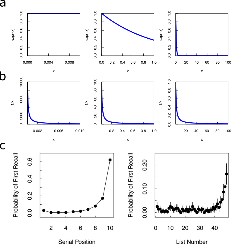
The recency effect refers to the finding that, all else equal, memory is better for information that was presented more recently. In free recall, this manifests as an increase in the tendency to initiate recall at the end of the list (Fig. 3) as well as higher probability of recall overall. The recency effect can be observed in all of the experimental paradigms that people study with human participants.
The recency effect is especially pronounced in immediate free recall, in which the recall test proceeds just after the last item in the list Murdock (1962). In delayed free recall, a delay interval is included during which participants typically perform a distractor task (to prevent them from simply repeating the items in the list to themselves) prior to recalling the words from the list. In delayed free recall the recency effect is sharply attenuated. However, the probability of recall of early items from the list is barely affected relative to immediate free recall Glanzer & Cunitz (1966); Postman & Phillips (1965). In contrast, many other variables (e.g., presenting the words faster or slower, choosing words that are semantically related, having medial temporal lobe amnesia) have a big effect on recall of items from the beginning and middle of the list, but barely any effect on the recency effect Glanzer (1972). These observations led researchers to propose that the recency effect draws on a specialized memory store, referred to as short-term store (STS) or short-term memory Atkinson & Shiffrin (1968); Raaijmakers & Shiffrin (1980).
The view that memory was divided into distinct stores was hugely influential in the 1970s and 1980s and remains so today. The basic idea (Figure 2a) is that STS can store a small number of items with very high accuracy. Items that are in STS at the time of test are recalled rapidly and with high precision. In addition, a subset of items are passed from STS to a long-term store (LTS). LTS does not have capacity limitations and can store information for a much longer duration. The longer an item spends in STS during study, the greater the probability it is transferred to LTS. A key property of STS is that it is subject to strategic control according to the goals of the participant. For instance, if participants are rewarded based on how many words starting with the letter q they correctly recall, we might assume that words that start with a different letter are less likely to enter STS and would be forgotten very quickly.
If one specifies a strategy for retaining information in STS it is straightforward to work out (or simulate, if the strategy is very complicated) the probability that an item is in STS at the time of test. For instance, suppose that each item in a long list enters STS with certainty displacing a random item in STS. If the short-term store can hold items, where is much smaller than the number of items in the list then the probability that an item already in STS is replaced by an incoming item . The probability that the item already in STS persists in STS after a new item enters STS is thus . At the end of a list of items, the probability that the th item is still in STS at the time of test is , leading to a recency effect. Note that although this function decays exponentially, recency due to STS has different properties than recency due to exponential weight decay (Eq. 6). First, the quantity that is decaying is a probability rather than a strength per se. This probability gives the proportion of trials where the item is available for recall from STS; on trials where the item is not available, there is zero probability of retrieval from STS. This is distinct from a situation where the weights give a small but reliable signal. Second, although the probability of any one item remaining in STS may be a decreasing function, it should be kept in mind that the number of items in STS depends only on its capacity (assuming the list has more than items).
One can similarly work out probabilities for the amount of time a word spends in STS (recall that the probability of transfer to LTS goes up with time spent in STS). Coupled with a specfication of LTS one can make predictions for many observable properties of memory retrieval resulting in a very detailed description of immediate and delayed free recall, including but not limited to the recency effect.
A major challenge to the two-store account of recency came from a modification to the free recall paradigm referred to as continual distractor free recall (CDFR). Recall that in immediate free recall the recall test follows shortly after the last item in the list. According to STS-based accounts the recency effect in immediate free recall happens because the items from the end of the list are still available in STS. In delayed free recall, a distractor task follows the last item on the list before the recall test. The recency effect is attenuated in delayed free recall. According to STS-based accounts, this is a consequence of the distractor task pushing list items out of STS. In CDFR, a distractor task follows each item in the list, not just the last item. Perhaps surprisingly, there is a pronounced recency effect in continual distractor free recall relative to delayed free recall Bjork & Whitten (1974); Glenberg et al. (1980). This finding was not predicted by the STS-based account of recency and is difficult to reconcile with an account of recency solely based on STS Davelaar et al. (2005); Lehman & Malmberg (2012).
2.2 The contiguity effect across delays
As a thought experiment, try the following memory experiment on yourself. Answer the following question: What did you most recently have for breakfast?33 3 If you are eating breakfast while reading this you can substitute the question What did you most recently have for dinner? Most people, when answering this question, do not merely generate a verbal response (e.g., “toast”) but experience a vivid recollection of the event in the process of answering the question. For instance, while writing this (in the afternoon) in answering the question about breakfast I spontaneously remembered where I sat down (kitchen table with the window to my right), the hopeful look on my dog’s face, and the news I read on my phone. I can take another moment and search my memory to vividly remember events that happened shortly before eating breakfast (putting the coffee on the stove, putting bread in the toaster) and shortly after (finishing my coffee in the backyard with my dog).
The “kind of memory” that supports vivid recollection of events from one’s life is referred to as episodic memory Tulving (1983). Episodic memory has been extensively studied over the last several decades. For the present purposes we note that episodic memory is believed to be closely related to a phenomenon referred to as the contiguity effect. In free recall, the contiguity effect (Fig. 3b) manifests as the finding that (all else equal) if a participant has just recalled a word from the list, the next word that participant recalls tends to come from a nearby position in the list Kahana (1996). In memory experiments with a probe (e.g., cued recall), the contiguity effect manifests as the finding that the probe tends to bring to mind other items that were close together in time. For instance in cued recall, when a participant recalls a word that was not the correct response to the probe, that erroneous word tends to come from a pair that was presented nearby in the list. The contiguity effect is not limited to experiments with words as stimuli and is indeed quite general Healey et al. (2018).
Note that the episodic memory for today’s breakfast illustrates the contiguity effect. Sitting down at the table, giving my dog a piece of sausage and reading about terrible events unfolding overseas were not actually simultaneous but were relatively close together in time (probably tens of seconds). The other events I retrieved – putting the bread in the toaster and finishing the coffee in the backyard – were each separated by several minutes from breakfast per se. Consistent with this intuition, the contiguity effect is observed in the laboratory in CDFR experiments where the items are separated by tens of seconds. The contiguity effect can also be observed over much longer time scales – hundreds of seconds in final free recall Howard et al. (2008), hours in experiments using mobile phones to administer a list as participants went through their daily lives Mack et al. (2017) and even much longer periods of time in retrieving news events Uitvlugt & Healey (2019).
One may think of the contiguity effect as analogous to the recency effect, but taken from a different temporal reference frame. The recency effect describes the availability of items in memory as a function of their temporal proximity to the present. In contrast, the contiguity effect describes the availability of items in memory as a function of their temporal proximity to a remembered moment from the past. This analogy between recency and contiguity suggested a different class of models for memory, which we turn to in the next subsection.
2.3 Temporal context models
In this subsection we describe the memory representations of a class of models referred to as temporal context models (Howard & Kahana (2002); Sederberg et al. (2008); Polyn et al. (2009), TCMs,). These models were originally developed to account for recency and contiguity effects in free recall. TCMs have since been applied to other episodic memory tasks, and even memory tasks that are not considered to tap episodic memory Logan (2021). In this subsection we will describe the basic properties of these models and how they result in properties of memory. We will discuss neuroscientific work inspired by TCMs before describing some fundamental limitations that follow from the form of temporal context.
Temporal context models make three important conceptual changes relative to the models we have considered thus far in this chapter. First, these models hypothesize a vector representation of temporal context that changes gradually from moment-to-moment. We will specify this in more detail below. For now, we note that the temporal context vector shares at least some features with the content of short term store. Second, temporal context models do not attribute behavioral associations between items – such as the contiguity effect – to direct connections formed between item representations (as in Eq. 1). Rather, functional associations in temporal context models are mediated by items’ effects on temporal context and a temporal context’s ability to cue retrieval of items. Third, temporal context models assume that it is possible to reinstate a previous state of temporal context. This “jump back in time” is hypothesized to be associated with the experience of episodic memory.
2.3.1 Two interacting vector spaces: items and contexts
In TCMs, there are two interconnected vector spaces (Fig. 2b). One vector space, which we will sometimes refer to as the item space, is activated by items that are currently available, either by virtue of having been presented by the experimenter or by virtue of having been recalled by the participant. We refer to the cognitive representation of specific items as vectors and the vector corresponding to the item presented at time step as . The other vector space, which we will sometimes refer to as the context space maintains a state of temporal context. We will refer to the state of temporal context at time as . Temporal context is affected by items; the input at time , is caused by , the item available at time .
Temporal context evolves gradually, retaining information contributed by recent items:
| (7) |
That is, at each time step , the new state of temporal context is given by times the previous state of temporal context, plus the input caused by , . As before, so that in some formulations, is allowed to vary as a function of time (for instance to normalize the context vector) and/or can vary for different components of the context vector as attention to different features changes (e.g., due to different encoding tasks). We assume that on the initial presentation of an item in a randomly-assembled list of words, the inputs caused by each item are uncorrelated with one another and treat them as random vectors. Equation 7 shows that information caused by a particular item persists after it is presented. Recursively unwinding Eq. 7 we find
| (8) |
That is, the input pattern caused by an item decays exponentially as additional items are presented.
At any particular moment, recall is cued by the current state of temporal context via an associative matrix that connects the context layer (containing context vectors ) to the item layer (containing item vectors ). Analogous to our simple Hebbian model (Eq. 1), the basic formulation provides an outer product association between the context available prior to presentation of the current item and the item itself
| (9) |
This shift in indices ensures that the temporal context that cues does not include information that item itself caused.
Equation 9 resembles Eq. 1 in that it associates two patterns via an outer product. However, rather than associating two items and , associates a context vector to an item vector. The context-to-item association means that a probe context activates each item in the list to the extent the probe context resembles that items’ encoding context. By analogy to Eq. 4,
| (10) |
Because context changes gradually, this typically results in a weighted sum of many items. Temporal context models use a retrieval rule to probabilistically select an item for recall. These mechanisms are sometimes quite elaborate; the key feature they share is that the probability of recalling a particular item at a particular retrieval attempt depends not only on the degree to which it is activated, but also on the activation of the other items in the list. That is to say, items compete to be retrieved.
2.3.2 Recency effect
We are in a position at this stage to understand why TCMs predict recency effects in immediate and delayed free recall. Combining Eq. 8 and Eq. 10 we find, under the assumption that the during initial study of a random list are orthorgonal to one another, that probing with the context available at the end of the list, , gives back the items from the list weighted exponentially:
| (11) |
The exponential decay clearly provides a large advantage to items from the end of the list, leading naturally to a robust recency effect. Introducing a delay takes , where the distractors ought to be orthogonal to the list items. This reduces the difference in activation between the last items in the list and earlier items, resulting in a decrease in the magnitude of the recency effect.
2.4 Contiguity effect
Thus far we have considered only the case where the input patterns caused by the items in the list are orthogonal to one another. In this subsection we study the effects of relaxing this assumption. To make the ideas clear, let’s repeat an item at the end of a very long list of unrepeated items and see how the resulting context cues the neighbors of the repeated item. We consider two possibilities. In the first case, the repeated item simply causes the same input that it did during the initial presentation of the list. In the second case we consider the case that the repeated item recovers the temporal context available when it was intially presented; that the repeated item causes a jump back in time. We will find that these two hypotheses result in very different qualitative properties.
Let us label the time index at which an item is repeated as , the position at which the repeated item was initially presented as and study the ability of to cue items near , . We assume that is far in the future so that we can neglect and restrict our attention to . Suppose that the repeated item simply causes the same input at time step that it did when it was initially presented at time step . Because persisted after time step (see Eqs. 7, 8), this results in similarity to the context states that followed time step . This similarity decreases exponentially with . Put another way, because temporal context contains information from recently presented items, is similar to the temporal context of items for which was in the recent past. However, the same is not true for items that preceded item . For , information retrieved by item is not in the recent past – item has not been presented yet and there is no way the participant should be able to predict a word in a random list. Putting these considerations together, we find that if :
| (12) |
That is, if at time step , the item at time step simply recovers the same input it caused during encoding, , this results in an asymmetric functional association to its the neighbors.
Now let’s consider the case in which the repeated item recovers the state of context available when it was initially presented, . This context includes information caused by the items that preceded item . This information also persists in temporal context after item was presented. Noting that the inner product is symmetric, , we conclude that in this case
| (13) |
That is to say, retrieving the previous state of temporal context results in a symmetric association that falls off exponentially as a function of .
In most free recall experiments, the shape of the contiguity effect includes a contiguity effect in both the backward and forward direction, with a reliable advantage for forward transitions (Fig. 3b is representative). In TCMs, the pattern retrieved by item when it is re-experienced at time step is a mixture of these two patterns:
| (14) |
The value of can be estimated from the data and is believed to vary not only from participant to participant but also from one retrieval to the next. This makes sense of the finding that episodic memory retrieval – presumably related to the recovery of a previous state of temporal context – does not always succeed. This property of episodic memory is familiar to anyone who has bumped into a familiar person in a public place (e.g., a grocery store) …but been unable to actually remember any details of the person’s actual identity.
2.5 Neural evidence for temporal context models
Temporal context models have benefitted from a relatively close connection to work in cognitive neuroscience. After all, if the long-term goal of this kind of modeling is to develop a more-or-less literal model of the computations that take place in the brain during memory encoding and retrieval it is essential to compare hypotheses to the activity of neurons in the brain. We briefly point to three pieces of evidence that speak to the utility of TCMs in making sense of human and also animal neuroscience.
First, the division of into two components with distinct properties (Eq. 14) has been very productive in explaining otherwise isolated findings in neuropsychology and cognitive neuroimaging. To take a simple example, imagine if it were possible to alter across experimental groups. A group with a lower value of ought to have difficulties with vivid episodic memory recall, but also show a more asymmetric contiguity effect in free recall. This finding has been observed with patients with medial temporal lobe amnesia Palombo et al. (2019), electrical stimulation to the entorhinal cortex Goyal et al. (2018), and participants who are experiencing cognitive declines with aging, perhaps leading to Alzheimer’s disease Quenon et al. (2015); Talamonti et al. (2021). Moreover, according to the models, retrieved temporal context ought to be preferentially involved in particular sorts of memory. Consider an experiment where participants learn pairs separated by long periods of time, absence hollow …hollow pupil. If the second presentation of hollow can cause recovery of its previous context (i.e., the caused by absence), then absence in effect becomes part of the temporal context for pupil. If , the model can still learn the pairwise associations using the forward part of the contiguity effect. Indeed, normal human participants generalize absence pupil associations even though absence and pupil were never experienced nearby in time. As it turns out, lesions to a brain region called the hippocampus – which is believed to be important in episodic memory – cause a deficit in these bridging or “transitive” associations in rodents while leaving the pairwise associations unaffected Bunsey & Eichenbaum (1996), just as if the hippocampus is responsible for causing a recovery of temporal context. A number of neuroimaging studies have studied similar experimental paradigms in humans, showing that the hippocampus and hippocampal-prefrontal interactions are important in these transitive associations Zeithamova et al. (2012).
One can also measure direct neural predictions from TCMs. The most characteristic prediction is the existence of a temporal context vector , which should show temporal autocorrelation extending over macroscopic periods of time – at least tens of seconds. One can construct a vector of brain activity using many different methods. For instance, it is practical to record simultaneously from many individual neurons at once. Taking the number of spikes for each of neurons averaged over, say, a one second interval gives an -dimensional vector. One can then compute a temporal autocorrelation function by comparing response vectors from neighboring time points. This type of analysis has shown robust evidence for signals that are autocorrelated over seconds, minutes, and even hours or days in a number of brain regions, notably the hippocampus and prefrontal cortex Mankin et al. (2012); Hyman et al. (2012); Cai et al. (2016). These studies have focused on rodents because of the array of systems neuroscience tools that can be brought to bear in rodents, but analogous results have been found with human fMRI Hsieh et al. (2014).
The most characteristic prediction of TCMs is that the state of temporal context should be recovered when an episodic memory is retrieved (Eq. 13). When item is repeated at some later time step , and causes an episodic memory, the context at time step should resemble the context prior to the context at time step . This is non-trivial; any neural information that was caused by item during study can only be observed after its original presentation. There is evidence from invasive human recordings of this phenomenon in several human memory paradigms Manning et al. (2011); Yaffe et al. (2014); Folkerts et al. (2018), fMRI studies of free recall Chan et al. (2017), and real-world memory extended over hours and days and weeks Nielson et al. (2015).
2.6 Memory is scale-invariant; exponential functions are not
In our discussion of models of short-term memory, we noted that the failure of short-term memory models to account for the long-term recency effect and long-term contiguity effects was a serious problem for those models. It is true that TCMs are better able to account for those phenomena. In STS-based models, the probability that an item is perfectly represented in STS falls off exponentially. As time passes, STS provides zero information about the item on an increasingly high proportion of trials. In contrast, in TCMs the information about an item falls off exponentially with time, but is reliable across trials. With a bit of resourcefullness and a few free parameters, one can exploit this property to provide a reasonable fit to experimental data from continuous distractor free recall. But this account is still theoretically unsatisfactory, as we shall see shortly.
As discussed above, a great deal of evidence suggests that recency and contiguity effects not only persist across a delay interval in CDFR, but are observable at an extremely wide range of time scales (Figure 4c provides a particularly striking example). This suggests that the memory representations governing recency and contiguity effects are scale-invariant Chater & Brown (2008). A function is said to be scale-invariant if it is unaffected by rescaling the input up to a scaling factor. That is, a function is said to be scale-invariant if stretching or compressing its input by a constant, , results in the same function up to a constant term that depends only on : . This property is true of power law functions that govern, say, electrical potential as a function of distance from a charged particle, or the gravitational field as a function of distance from a massive object in Newtonian gravity. We can easily convince ourselves of this property by noting that if , then , satisfying the constraint. Figure 4b illustrates this property for by rescaling the axis.
The exponential functions generated by TCMs are decidedly not scale-invariant. Note that if we choose . More generally, if so that . Thus, choosing a is equivalent to specifying a rate constant (or a time constant ) for an exponentially decaying function. Figure 4a shows the function rescaled over the same range of values as the power law function. When is much less than one (left panel), the exponential function appears linear. This follows from the Taylor series expansion of the exponential function:
| (15) |
where additional terms include higher powers of multiplied by . As we zoom out (right panel), the exponential function comes to approximate a delta function centered at zero. Note that in both of these two regimes and , the exponential function is useless for expressing a recency effect. Mapping to recency, when is small, there is no forgetting because all points are associated with a high nearly constant value. When is large, almost all points (excluding zero) are mapped to a low nearly constant value.
This rescaling is not an academic exercise. CDFR approximates rescaling of experience. Insertion of a delay of duration between each item and at the end of the list approximates taking , so that the relative delay between serial positions relative to the time of retrieval becomes effectively larger. From this it is clear that, although one may be able to approximate experimental data in restricted cases, the machinery of the temporal context vector specified by Eq. 7 is not scale-invariant and will eventually break down.
3 Scale-invariant temporal history
Thus far, we have considered models based on more or less complicated implementations of the idea of association. In the case of the Hebbian association model, the association is distributed across the entries in a matrix corresponding roughly to the set of synapses between items. In temporal context models, associations between items are mediated by temporal context, a representation of the recent past in which previous events decay gradually. These models share an implicit assumption that the goal of memory is to express relationships as a scalar value. That is, we can talk about the relationship between, say absence and hollow only in terms of the magnitude of the connection between them. Given two pairs, absence—hollow and pupil—river, the simple Hebbian model does not have any mechanism to convey information about whether one pair was learned before or after the second pair. Yes, one might note that the absence—hollow association is stronger than the pupil—river association and use this to infer that absence—hollow was more recent, but this inference would break down if, for instance, the participant was paying less attention when pupil—river was presented, or if absence—hollow was presented multiple times.
Similar arguments apply to TCMs. Although temporal relationships can be inferred indirectly from the magnitude of the associations between multiple words, there is no explicit information about the direction of time contained in . Consider two context vectors and . The direction of the difference between these two vectors, , depends on the particular choice of items presented during the interval specified by lag rather than the time per se. Moreover, as with simple Hebbian models, repeated items can make even the magnitude of these vectors ambiguous. The goal of the representation used in this section is to build a replacement for the temporal context vector. We desire that this representation carries explicit information about temporal relationships. We also desire that this representation can be used to build scale-invariant models of memory.
Understanding vectors as activated populations of neurons, the simple Hebbian model and temporal context vectors distribute “what” information about the stimuli that are experienced across populations of neurons. Different basis vectors of the space correspond to different properties of stimuli. The temporal context vector provides decaying “what” information “smeared” over the recent past. The strategy of this approach is to construct a population of neurons that not only represent information about what has happened in the recent past, but to distribute information about when it happened across different neurons. That is, our computational goal is to estimate the recent past as a function of time. Figure 5 provides an illustration and introduces notation. In this section we describe a specific solution to this problem that has found considerable empirical support from data from both psychology and neuroscience.
Let us suppose that the world provides a continuous stream of input . Like the set of vectors corresponding to a list of words, is in general vector-valued but we will suppress vector notation for now. Consider the problem of an observer having examined up to a particular point . We will refer to the history leading up to this moment as , where runs from zero to and corresponds to the present. Our goal is to construct an estimate of the history leading up to time as . We desire that this estimate approximates reality – with error that is comparable across time scales – and is also a computation that could be implemented by neural circuits. The next subsection introduces a specific method that has these properties (Shankar & Howard (2012), proposed by). Subsequent subsections demonstrate that it is straightforward to build not only temporal context models out of this form of representation but other more “cognitive” models as well. Finally, we touch on a wealth of neuroscience work that suggests that populations of neurons like those proposed for .
| a | b | ||
|---|---|---|---|
 |
 |
3.1 Estimating temporal relationships using the Laplace transform
This section describes a method for estimating based on Laplace transforms that was proposed by Shankar & Howard (2012). First let us write a continuous version of Eq. 7. For reasons that will become clear, we change notation such that the temporal context vector is written as and the input to the context vector is written as . We take both of these to be vector-valued but will suppress the vector notation for present. Defining , this is just a continuous version of Eq. 7:
| (16) |
Solving Eq. 16 we find, in the general case:
| (17) |
Comparing this to Eq. 8 we see a close correspondence between and if we make the identification . In contrast to the TCMs we discussed in section 2.3, we do not understand as a parameter to be estimated from the data of a particular experiment, but as a continuous variable. To be concrete, we can imagine that we have an ensemble of units, each with a different value of .
3.1.1 Continuous enables information about continuous time
Treating as a continuous variable allows us to reconstruct information about the value of at different values of . With any particular value , captures information about the past history up to a time scale on the order of . If we chose a different value , would capture information up to . For simplicity, lets assume that . Consider the properties of the exponential function illustrated in Figure 4. For values of much less than , both and weight by similar amounts. Similarly, for values of much greater than , both of the exponential functions have decayed to zero and neither nor carries information about in that interval. However, consider how the two values of vary as increases from to (recall that ). As passes through , the contribution of to rapidly decreases. However, the exponential for decays less steeply in this region, so that the contribution of these values to is greater. We conclude that one can infer something about the values of in a region specified by and by observing the difference between and . Given many values of we can infer at many values of .
More formally, we can note that from Eq. 17 describes the real Laplace transform of . The Laplace transform is invertible; if we know the value of precisely with every real value of from 0 to , then we can specify precisely for every value of from 0 to . We will restrict our attention to real positive values of .44 4 Negative real values of would be neurally unreasonable. We ignore complex for simplicity.
3.1.2 Approximately inverting the Laplace transform
Now that we’ve established that carries information about the time of past events , we need to determine how to extract that information. Knowing that is the real Laplace transform of suggests a strategy – simply invert the Laplace transform. That is, provides a memory for the past leading up to the present . After inverting the Laplace transform, we would obtain an estimate of the actual history, which we write as . Over the years, many methods for the inverse Laplace transform have been proposed. We focus on the Post approximation Post (1930), which is relatively straightforward to implement in neural circuits and has some computational properties that are advantageous in describing psychological and neurophysiological results.
To approximately invert the transform, we define a mapping , where is an integer to be approximated from the data. At each moment, the value of at each value of is computed as
| (18) |
The derviative on the right hand side is to be taken in the neighborhood of the value of . is a constant that ensures that the sign and magnitude of corresponds to the sign and magnitude of . The operator includes a computation of the th derivative with respect to .55 5 Given a discrete set of values, can be understood as a matrix that maps onto , with a matrix implementation of the discrete derivative. In the limit as , the Post approximation becomes the inverse transform and . However, for finite , there is a temporal blur introduced. is equal to an average of in the neighborhood around . Suppose is a delta function at a particular time in the past. Then
| (19) | |||||
| (20) | |||||
| (21) |
The constant includes a factor of so that the right hand side of this expression is positive for all . The function on the right-hand side of Eq. 21 is a product of a growing power law and a decreasing exponential, resulting in a function that has a single peak. Freezing time at a particular and looking across all , the peak comes at . Fixing a particular and observing it through time as changes, the peak comes at . The most important property of this expression is that the right hand side depends on the time only through ratio . Because of the linearity of Eq. 17 and the linearity of , we can write an expression for any history as
| (22) | |||||
| (23) | |||||
| (24) |
Where we have defined and changed variables to in the last line.
3.1.3 A note on biological realism
As we will see later, these equations provide a reasonable description not only of a memory representation that can be used to describe behavior in a range of memory tasks, but also of neurophysiological data from a number of brain regions. The equations are in principle computable by neurons – Eq. 16 simply requires slow time constants and it has long been known that the brain can compute derivatives needed to implement . How literally should one take these equations? There is certainly a level of precision at which these equations are not a correct description of the firing rate of neurons. The author of this chapter encourages the reader to take these equations seriously, but not literally.
For instance, Eq. 16 describes an instantaneous reaction to an input in continuous time. If one understands as a stimulus under external control this cannot be literally true. Moreover, there are a number of ways in which the brain could implement the slow rate constants in Eq. 16, including recurrent connections, metabotropic glutamate receptors Guo et al. (2021) and feedback loops between spiking and intrinsic currents Egorov et al. (2002); Tiganj et al. (2015). These mechanisms would all have slightly different properties that would deviate from Eq. 16. However the larger point that firing for a population of neurons decays roughly exponentially following a triggering stimulus with a broad range of time constants may still be true.
Similarly the inverse operator cannot be literally true. One major issue is that is a linear operator. Taken literally, linearity of the right hand side of Eq. 18 would require that every bit of information about the change in is reflected, at least a little bit, in , which seems unreasonable. Another serious problem is that empirical values of estimated from neural data can be quite high Cao et al. (2021). This is a computational problem in that computing the th derivative becomes more and more sensitive to noise as increases Shankar & Howard (2012). In real cortical circuits, recurrent feedback involving networks of inhibitory interneurons works to dampen noise Ferster & Miller (2000). Nonetheless, captures some important phenomena of neural firing that should be taken seriously. First, the weights of do not reflect any type of learning or experience with the stimuli. They only extract information embedded in a population with different decay rates. Second, the shape of the receptive fields predicts for seem to agree reasonably well with experiment Howard et al. (2014), at least in cases with a few discrete stimuli presented widely separated in time. Third, the idea of using derivatives with respect to as a signal to infer the time of a stimulus presentation is a sound idea, even if the brain doesn’t literally use the Post approximation with (or some other very large value of ) to extract this information.
3.1.4 A logarithmic scale for past time
Note that although Eq. 23 is written as an integral transform of , it is not necessary to retain a detailed memory of . Updating Equation 16 requires only the preceding value and the momentary value ; there is no need to retain prior values of above and beyond the information present in . Moreover can be computed from . We thus have a choice to make about how much information to retain in . That is, the brain can’t actually have an infinite number of values of . And there is no reason a priori to assume that the values that are sampled should be evenly spaced. Because , choosing how to distribute the also specifies how to distribute the . Equations 23 and 24 suggest a specific choice for sampling .
Consider at two nearby values of , which we’ll refer to as and . If we observe and find that it is at a high value, we know that is also likely to be at a high value. Conversely, if we observe that is close to zero, we know that is also likely to be close to zero. Because they are affected by nearby points in time, these two values of are correlated with one another. Each value of we sample costs us something (e.g., metabolic energy for a brain, availability of RAM in a computer simulation, etc). In the limit as , there is no benefit to measuring at a second value. As increases from zero, the two values of provide different information about the past and there is some benefit to counteract the cost of sampling a second value of . However, the benefit from a particular number depends on the choice of the first . To get an intuition into why this is so, suppose that we start with a specific and specific , then we vary while keeping fixed. As we increase , the impact of a fixed value of becomes less and less. This is true because in Eq. 23 depends only on the ratio and the difference between and grows smaller as increases for all . If we adopt the strategy of choosing so that each additional value of provides the same benefit, we arrive at a sampling strategy where the difference between adjacent values of goes up linearly with the value . One can formalize this further.66 6 For instance, it can be shown that if is driven by white noise, the mutual information between two values of sampled over time depends on the ratio of their s (Shankar & Howard (2013), see Appendix A.1 of).
Setting the spacing between adjacent samples of to be proportional to the starting value of leads immediately to several properties. First, the ratio between adjacent values must be a constant,
| (25) |
Second, the number of units one observes with a particular value of should go down with that value of :
| (26) |
This expression diverges at zero, which is obviously not physical. One solution is to fix some minimum value of that can be sampled .77 7 If it is important to sample zero, one could use some other sampling scheme for values below some threshold in order to arrive at zero Howard & Shankar (2018). Third, the samples of are evenly spaced as a function of the logarithm of :
| (27) | |||||
| (28) |
This cluster of properties are quite theoretically satisfying. Many sensory receptors in the mammalian brain sample continuous dimensions at logarithmically spaced intervals. For instance, the density of receptors on the retina has long been known to decrease linearly with distance from the center of the retina, as in Eq. 26, a property that appears to be respected throughout early stages of the visual system in the brain. Psychologically, the logarithmic sampling of time (Eq. 28) provides a close correspondence with the Weber-Fechner law from psychophysics, which states that the magnitude of a perceptual variable goes up linearly with the logarithm of the physical stimulus that causes it. The Weber-Fechner law holds (at least approximately over some range) for a number of simple stimulus dimensions (e.g., loudness of a tone, pitch of a tone, length of lines, etc) and has been argued to hold for perception of temporal intervals as well. It would be quite elegant if the brain distributes receptors along a time axis using the same mathematical expression as receptors along the retina, resulting in a similar perceptual invariance. It is especially satisfying that the arguments leading to logarithmic distribution of “time receptors” made no reference to these data. Rather, Eqs. 25-28 were derived from a property of the Post approximation coupled with the argument that the brain ought to equalize redundancy among the receptors.
3.2 Behavioral models using scale-invariant temporal history
The scale invariant temporal history described in section 3.1 can be used to construct a wide variety of behavioral models of memory. It is straightforward to extend temporal context models by using in place of . The primary result is that one obtains scale-invariant recency and contiguity effects (Fig. 4). However, the temporal history can also be used to construct computational models of very different tasks that can not be readily modeled using temporal context models. Some of these tasks are believed to rely on different “kinds of memory” than free recall.
3.2.1 Scale-invariant temporal context models
TCMs rely on the temporal autocorrelation of the temporal context vector in order to generate recency and contiguity effects – that is, even in a list of random words, the expectation of falls off gradually like . However, exponential functions set a strong scale. One can readily build a temporal context model using in place of . Rather than associating context vectors to items, one constructs an associative matrix for each :
| (29) |
Recall that at a particular is essentially a temporal context vector with . If one imagines as the matrix one would get for each value of as a function of , then is just that matrix valued function of , but with the inverse transform applied.88 8 The transform here would be applied from the right: . One may visualize for a particular as a set of connections between a particular row in Figure 5b and the vector . One obtains a probe as . Each list item is activated to the extent that the units in the temporal history when it was presented are also active in the probe. One may visualize this operation with respect to Figure 5b as follows. When a particular item is activated in , there is a particular pattern . That item is activated according to the match between and the probe , summing over rows (corresponding to the inner product) and columns (corresponding to the sum over ). In the case of a long list of non-repeating words, it can be shown that this association falls off like a power law function Howard et al. (2015). This property makes TCMs built in this way scale-invariant. It is thus straightforward to build genuinely scale-invariant recency and contiguity effects.
TCMs built from a scale-invariant temporal history also have qualitatively different properties than TCMs that use only a single-scale temporal context vector. Consider a situation in which two items, a and b are presented at a temporal separation of seconds. The temporal context for b has a presented seconds in the past. Let us repeat a and observe the prediction for b as a recedes into the past. First, in the case of a single temporal context vector, the temporal context for b is just . When a is repeated (neglecting retrieval of temporal context) it again contributes a term to the temporal context vector and b is cued by an amount proportional to . But now consider what happens in the time after a was repeated. In the time following repetition of a, the magnitude of the component of the temporal context vector decreases exponentially. As a consequence b is cued less and less as a recedes into the past after its repetition. The behavior is very different if temporal context is constructed from . As before, the temporal context that cues b is the representation of a presented seconds in the past. However, this corresponds to an in which units triggered by a with near are active. When a is repeated (again neglecting recovery of temporal context), it again triggers a sequence of cells. A time after repeating a, the units with near are active. But if , these are different units than the ones that cue b. As the repetition of a recedes into the past, b is cued more as approaches and then less as the sequence passes through the units that form the temporal context for b. Although the consequences of this property on models of free recall would be expected to be relatively subtle (there are many items composing the temporal context and retrieval of temporal context), this property could be extremely useful in other behavioral applications (e.g., serial recall).
3.2.2 Probing a representation of what happened when
The simple Hebbian model described in section 1 is a special case of a class of distributed memory models called global match models. The name “global match” refers to the property that the probe is compared to one composite memory that contains a mixture of information from all of the items in memory. Other distributed memory models made different assumptions. For instance, multitrace models (D.L. Hintzman (1984); Shiffrin & Steyvers (1997), e.g.,) assumed that memory is composed of a list of traces which can be selectively accessed based on the probes one provides as part of a query of memory. Each trace is a set of features stored at a particular time, closely analogous to in the simple Hebbian model and TCMs.
The temporal context model sketched above using as a probe has the spirit of a global match model. One builds an associative and then takes a sum over both what and when information in constructing the output of memory, . However, there are other ways one might query to construct behavioral models of different memory tasks. Multitrace models keep different elements of memory separate in a list. Because it maintains separable information about what happened when, one can understand as a multitrace model, albeit one where the traces become more blurred together as time recedes into the past (Figure 5b). Behavioral modeling work has shown that by querying this representation in different ways, it’s possible to construct quantitative behavioral models of different working memory tasks.
It is well established that people and animals can direct attention to a restricted region of visual space. Suppose that a participant maintains fixation at a particular spot in a visual display for a few seconds (in experiments a small spot is usually provided). Now suppose that the participant learns that something important will be presented in a particular region above and to the left of the location that is being fixated. It can be shown that the ability to perceive visual information is greater if a stimulus is presented in that region relative to a region where nothing in particular is expected. This increased perceptual and neural gain is referred to as “attention”.
One can model attention, directed to particular regions of past time; this capability is important in constructing behavioral models of working memory tasks. Let us suppose that one can direct attention to particular regions of the timeline and then compute a vector-valued output like so:
| (30) |
Here is an attentional weight that can highlight the contributions of items at different points in the past. It is not reasonable to suppose that attention can take the form of any arbitrary function over . Let us suppose three constraints on the form of attention. First, attention can point at only one circumscribed region at a time. The function for attention should have one peak at a particular index . Second, attention can be deployed over a wide region or a more narrow region depending on the task demands. To be concrete, given that attention is directed to a particular index , one may imagine that the participant can control whether attention extends to many nearby indices, falling off gradually, or only extends to a few nearby indices, falling off more sharply. Notice that because of the spread in over (e.g., see Fig. 5b), even if attention was nonzero for exactly one index , this would still allow information from nearby time points to contribute to . These simple assumptions allow us to construct very different behavioral models from the same memory representation.
This flexibility is useful in modeling working memory tasks. Working memory is a term used to describe a form of memory that stores information with high precision for a short time. Working memory is an intellectual descendent of computational models based on STS and is believed to rely on brain regions distinct from the regions responsible for episodic memory tasks like delayed and continuous distractor free recall. The first of these working memory tasks is referred to as probe recognition; the second is judgment of recency (JOR). In both tasks, the participant is presented with a short list of highly-memorable stimuli – to be concrete let’s assume that the stimuli are letters of the alphabet presented visually on a computer screen. In both tasks, the lists are relatively short (say 10 items) and the memory test is given immediately. In both tasks, the stimuli are repeated many times over an experimental session lasting tens of minutes. In both tasks, the participant is given a probe consisting of letters for the memory test. The only (important) way the tasks differ is in the judgment the participant must make in response to the memory probe. In probe recognition, the participants’ job is to press a button to indicate whether a probe stimulus was in the most recent list or not. Because the stimuli are repeated across many lists, the task is really to judge whether the probe was presented in a relatively broad region of time. In the short-term JOR task, participants are given a pair of probe stimuli and asked to select the probe stimulus that was presented more recently. Because both of the probe items came from the most recent list, short-term JOR requires more fine-grained judgments of the temporal record of the probe stimuli.
Although the details are beyond the scope of this chapter Tiganj et al. (2019), a carefuly study of accuracy and the amount of time it takes participants to respond shows that although both tasks show a robust recency effect, the manner in which memory is accessed is quite different. The findings from both experiments can be accomodated by models in which one makes a decision based on how well a probe overlaps with , . The important difference between the model for probe recognition and JOR is how attention is deployed. In the model of probe recognition, attention is deployed broadly such that it’s constant over the list. The overlap with the probe is thus stronger for more recent items and this strength falls off like a power law (Eq. 23). This provides a respectable model of probe recognition (Donkin & Nosofsky (2012), see especially). In short-term JOR the pattern of results has long suggested that participants use what’s called a self-terminating serial scanning model. We can build a serial scanning model over the scale-invariant temporal memory by supposing that the participant first sets attention to the recent present, such that only is one. The participant then compares this output to the memory probes. After some very brief time, attention is shifted to a slightly less recent time point, for instance only is non-zero. The decision terminates when a match is found. One can visualize this process with the help of Figure 5b. After studying the list g k l n t x h suppose the correct answer is x. The participant will not find a match to x looking at the first several rows. The amount of time it takes to find a match and initiate a decision depends on how far in the past x was presented. If instead the correct answer was t one would have to scan over a longer distance to find information about that probe, predicting a correspondingly longer response time. There are many more detailed quantitative predictions that follow from these models that can be worked out.
The important point here is that it is only possible to construct such distinct behavioral models because has separable information about what happened when. If the information about the time of past events was stored as a single number, as in the temporal context vector, it is much more difficult to imagine an attentional model, and certainly not one that aligns as well to our current understanding of visual attention.
3.3 Evidence for scale-invariant temporal history in the brain

Taken literally, specifies the properties of a population of neurons. There is now extensive evidence for these predictions; populations of neurons referred to as “time cells” behave much as one might expect if they were implementing . Let us take literally – as a description of the firing rate of a population of neurons, each indexed by a particular value of . Time cells have now been observed in rodents Pastalkova et al. (2008); MacDonald et al. (2011); Mello et al. (2015); Tiganj et al. (2017) and non-human primates Jin et al. (2009); Tiganj et al. (2018); Cruzado et al. (2020) and have even received preliminary support from studies in humans Umbach et al. (2020). Although the label “time cells” is most frequently applied to neurons in the hippocampus, populations with similar properties have been observed in a variety of prefrontal regions as well as striatum. These regions are believed to support different forms of memory. For instance, hippocampus is believed to support episodic memory, prefrontal regions are believed to support working memory, and striatum is believed to support implicit memory. If indeed different regions supporting different kinds of memory show firing consistent with properties of , then this supports the hypothesis that behavioral models for different kinds of memory all rely on the same form of representation.
Consider how cells representing would change their firing as a function of time following a delta function input at . Each cell would start with a firing rate near zero. As approaches each cell’s value of , the firing rate of that cell would begin to increase, and then decrease again as becomes much larger than that cell’s . Different cells have different values of , so cells in the population would fire in sequence. The duration each cell spends firing depends linearly on its value of ; cells that fire later in the sequence should also fire for a longer time. Moreover, s are sampled evenly over rather than linear time, resulting in a decreasing number of cells that peak later in the sequence. Moreover, if the population carries information about what happened when, different stimuli should trigger distinguishable sequences. All of these properties have been quantitatively demonstrated in multiple brain regions, including hippocampus and prefrontal regions in monkey and rodent. Moreover, time cells are observed in a wide variety of behavioral tasks MacDonald et al. (2011); Tiganj et al. (2017); Tiganj et al. (2018); Cruzado et al. (2020); Mello et al. (2015); Jin et al. (2009), including in cases where the animal is given no task at all, but simply passively observes stimuli Goh (2021).
 |
 |
More recently, populations of neurons with properties like those predicted for have been observed in a brain region called the entorhinal cortex Tsao et al. (2018); Bright et al. (2020). Because they so closely resemble components of the temporal context vector (Eq. 7), these kinds of cells have been dubbed temporal context cells. The entorhinal cortex provides the major projection to the hippocampus, where time cells were initially characterized. Decades of neurophysiology, neuropsychology and cognitive neuroscience have implicated the entorhinal cortex and hippocampus in human episodic memory. For instance, the famous amnesia patient Henry Molaison (known prior to his death as H.M.) had bilateral damage to both the hippocampus and entorhinal cortex. Thus, a population of temporal context cells, which resemble , project to a population of time cells, which resemble in regions essential to human episodic memory.
3.4 Going forward
The convergence between theoretical considerations (section 3.1), behavioral models of memory (section 3.2) and neurophysiological findings (section 3.3) seems very unlikely to happen by chance. This formalism could provide a foundation on which to build models of behavior and cognition that are more or less literal descriptions of the computations taking place in the brain. Although a foundation may exist, the work of constructing a complete theory of memory in the brain has barely begun. Thus far, the behavioral models that have been developed are sketches of important effects. A complete theory would require that these models be fleshed out to provide a detailed description of behavior (like the models in section 2). Development of such a theory would also require careful neuroscientific studies across species and tasks informed by these quantitative models of behavior. Theoretically, the formalism for encoding and inverting the Laplace transform of functions of time can be extended to representing functions over other variables. In this way it may prove possible to connect computational models of memory to well-developed computational models for spatial navigation, perception and simple decision-making informed by neurobiological data.
4 Related literature
This chapter necessarily touched on only a tiny fraction of the data and computational models that have been used to understand human memory over the years. Kahana (2012) provides a thorough introduction to behavioral models of memory and important quantitative data from all the major human memory paradigms.
Stimulus sampling theory is much more rich than decribed in this chapter. It was rigorously developed by many researchers, with Stanford University providing a focal point in the 1960s. Students interested in stimulus sampling theory should consider the following papers Atkinson & Estes (1962); Bower (1967).
Atkinson & Shiffrin (1968) is a modeling tour de force applying STS-based behavioral models to many variants of cued and free recall. It should be considered required reading for mathematical psychologists interested in modeling behavioral memory data. Raaijmakers & Shiffrin (1980) is a remarkably detailed desription of serial position effects in free recall that relies heavily on “fixed list context,” an important concept in models of this era that is not discussed here (Criss & Shiffrin (2005), see also).
Howard (2018) provides a high-level review of cognitive and neural data related to the scale-invariant temporal history discussed in section 3 (Howard & Hasselmo (2020), see also). Howard et al. (2015) built a number of simple cognitive models of behavioral tasks corresponding to different “kinds of memory” and note how this representation relates to distributed memory models. Lashley (1951) provides an eloquent critique of the limitations of simple associations in describing memory that seems to anticipate many of the properties of (James (1890), see also). There are also interesting connections between the logarithmic temporal scale derived for time here and measurement theory in mathematical psychology (Luce & Suppes (2002), for an overview see) and exponential generalization Shepard (1987).
References
- Anderson ((1972)) Anderson, J.A. (1972). A simple neural network generating an interactive memory. Mathematical Biosciences 14 197-220.
- Anderson ((1973)) Anderson, J.A. (1973). A theory for the recognition of items from short memorized lists. Psychological Review 80 417-438.
- Atkinson & Estes ((1962)) Atkinson, R.C. & Estes, W.K. (1962). Stimulus sampling theory (No. 48). : Citeseer.
- Atkinson & Shiffrin ((1968)) Atkinson, R.C. & Shiffrin, R.M. (1968). Human memory: A proposed system and its control processes. In K.W. Spence & J.T. Spence (Eds.), The psychology of learning and motivation ( 2, p. 89-105). New York: Academic Press.
- Baddeley & Hitch ((1977)) Baddeley, A.D. & Hitch, G.J. (1977). Recency reexamined. In S. Dornic (Ed.), Attention and performance VI (p. 647-667). Hillsdale, NJ: Erlbaum.
- Balsam & Gallistel ((2009)) Balsam, P.D. & Gallistel, C.R. (2009). Temporal maps and informativeness in associative learning. Trends in Neuroscience 32 2 73–78.
- Bjork & Whitten ((1974)) Bjork, R.A. & Whitten, W.B. (1974). Recency-sensitive retrieval processes in long-term free recall. Cognitive Psychology 6 173-189.
- Bolkan et al. ((2017)) Bolkan, S.S., Stujenske, J.M., Parnaudeau, S., Spellman, T.J., Rauffenbart, C., Abbas, A.I.Kellendonk, C. (2017). Thalamic projections sustain prefrontal activity during working memory maintenance. Nature Neuroscience 20 7 987–996.
- Bower ((1967)) Bower, G.H. (1967). A multicomponent theory of the memory trace. In K.W. Spence & J.T. Spence (Eds.), The psychology of learning and motivation : Advances in research and theory ( 1, p. 229-325). New York: Academic Press.
- Bright et al. ((2020)) Bright, I.M., Meister, M.L.R., Cruzado, N.A., Tiganj, Z., Buffalo, E.A. & Howard, M.W. (2020). A temporal record of the past with a spectrum of time constants in the monkey entorhinal cortex. Proceedings of the National Academy of Sciences 117 20274-20283.
- Bunsey & Eichenbaum ((1996)) Bunsey, M. & Eichenbaum, H.B. (1996). Conservation of hippocampal memory function in rats and humans. Nature 379 6562 255-257.
- Bush & Mosteller ((1951)) Bush, R.R. & Mosteller, F. (1951). A mathematical model for simple learning. Psychological Review 58 313-323.
- Cai et al. ((2016)) Cai, D.J., Aharoni, D., Shuman, T., Shobe, J., Biane, J., Song, W.Silva, A. (2016). A shared neural ensemble links distinct contextual memories encoded close in time. Nature 534 7605 115–118.
- Cao et al. ((2021)) Cao, R., Bladon, J.H., Charczynski, S.J., Hasselmo, M. & Howard, M. (2021). Internally generated time in the rodent hippocampus is logarithmically compressed. bioRxiv 2021.10.25.465750 .
- Chan et al. ((2017)) Chan, S.C., Applegate, M.C., Morton, N.W., Polyn, S.M. & Norman, K.A. (2017). Lingering representations of stimuli influence recall organization. Neuropsychologia 97 72–82.
- Chater & Brown ((2008)) Chater, N. & Brown, G.D.A. (2008). From universal laws of cognition to specific cognitive models. Cognitive Science 32 1 36-67. doi:10.1080/03640210701801941
- Criss & Shiffrin ((2005)) Criss, A.H. & Shiffrin, R.M. (2005). List discrimination in associative recognition and implications for representation. Journal Experimental Psychology: Learning, Memory and Cogntion 31 6 1199-212. doi:10.1037/0278-7393.31.6.1199
- Cruzado et al. ((2020)) Cruzado, N.A., Tiganj, Z., Brincat, S.L., Miller, E.K. & Howard, M.W. (2020). Conjunctive representation of what and when in monkey hippocampus and lateral prefrontal cortex during an associative memory task. Hippocampus 30 1332-1346.
- Davelaar et al. ((2005)) Davelaar, E.J., Goshen-Gottstein, Y., Ashkenazi, A., Haarmann, H.J. & Usher, M. (2005). The demise of short-term memory revisited: empirical and computational investigations of recency effects. Psychological Review 112 1 3-42.
- Deitch et al. ((2020)) Deitch, D., Rubin, A. & Ziv, Y. (2020). Representational drift in the mouse visual cortex. bioRxiv .
- Donkin & Nosofsky ((2012)) Donkin, C. & Nosofsky, R.M. (2012). A power-law model of psychological memory strength in short- and long-term recognition. Psychological Science . doi:10.1177/0956797611430961
- Ebbinghaus ((1885/1913)) Ebbinghaus, H. (1885/1913). Memory: A contribution to experimental psychology. New York: Teachers College, Columbia University.
- Egorov et al. ((2002)) Egorov, A.V., Hamam, B.N., Fransén, E., Hasselmo, M.E. & Alonso, A.A. (2002). Graded persistent activity in entorhinal cortex neurons. Nature 420 6912 173-8.
- Eichenbaum ((2017)) Eichenbaum, H. (2017). On the integration of space, time, and memory. Neuron 95 5 1007-1018. doi:10.1016/j.neuron.2017.06.036
- Estes ((1950)) Estes, W.K. (1950). Toward a statistical theory of learning. Psychological Review 57 94-107.
- Estes ((1955)) Estes, W.K. (19551). Statistical theory of distributional phenomena in learning. Psychological Review 62 369-377.
- Estes ((1955)) Estes, W.K. (19552). Statistical theory of spontaneous recovery and regression. Psychological Review 62 145-154.
- Ferster & Miller ((2000)) Ferster, D. & Miller, K.D. (2000). Neural mechanisms of orientation selectivity in the visual cortex. Annual Review of Neuroscience 23 1 441–471.
- Folkerts et al. ((2018)) Folkerts, S., Rutishauser, U. & Howard, M. (2018). Human episodic memory retrieval is accompanied by a neural contiguity effect. Journal of Neuroscience 38 4200-4211.
- Gallistel & Gibbon ((2000)) Gallistel, C.R. & Gibbon, J. (2000). Time, rate, and conditioning. Psychological Review 107 2 289-344.
- Gibbon ((1977)) Gibbon, J. (1977). Scalar expectancy theory and Weber’s law in animal timing. Psychological Review 84 3 279-325.
- Gillund & Shiffrin ((1984)) Gillund, G. & Shiffrin, R.M. (1984). A retrieval model for both recognition and recall. Psychological Review 91 1-67.
- Glanzer ((1972)) Glanzer, M. (1972). Storage mechanisms in recall. In K.W. Spence & J.T. Spence (Eds.), The psychology of learning and motivation (p. 129-193). New York: Academic Press.
- Glanzer & Cunitz ((1966)) Glanzer, M. & Cunitz, A.R. (1966). Two storage mechanisms in free recall. Journal of Verbal Learning and Verbal Behavior 5 351-360.
- Glenberg et al. ((1980)) Glenberg, A.M., Bradley, M.M., Stevenson, J.A., Kraus, T.A., Tkachuk, M.J. & Gretz, A.L. (1980). A two-process account of long-term serial position effects. Journal of Experimental Psychology: Human Learning and Memory 6 355-369.
- Goh ((2021)) Goh, W.Z. (2021). Remembering the past to predict the future: A scale-invariant timeline for memory and anticipation . : Boston University.
- Goyal et al. ((2018)) Goyal, A., Miller, J., Watrous, A.J., Lee, S.A., Coffey, T., Sperling, M.R.others (2018). Electrical stimulation in hippocampus and entorhinal cortex impairs spatial and temporal memory. Journal of Neuroscience 3049–17.
- Guo et al. ((2021)) Guo, C., Huson, V., Macosko, E.Z. & Regehr, W.G. (2021). Graded heterogeneity of metabotropic signaling underlies a continuum of cell-intrinsic temporal responses in unipolar brush cells. Nature Communications 12 1 1–12.
- Hasselmo & McClelland ((1999)) Hasselmo, M.E. & McClelland, J.L. (1999). Neural models of memory. Current Opinion in Neurobiology 9 184-188.
- Hasselmo & Wyble ((1997)) Hasselmo, M.E. & Wyble, B.P. (1997). Free recall and recognition in a network model of the hippocampus: simulating effects of scopolamine on human memory function. Behavioural Brain Research 89 1-2 1-34.
- Healey et al. ((2018)) Healey, M.K., Long, N.M. & Kahana, M.J. (2018). Contiguity in episodic memory. Psychonomic bulletin & review 1–22.
- D. Hintzman ((1987)) Hintzman, D. (1987). Recognition and recall in minerva 2: Analysis of the ‘recognition-failure’ paradigm. In P. Morris (Ed.), Modelling cognition (p. 215-229). New York: Wiley.
- D.L. Hintzman ((1984)) Hintzman, D.L. (1984). MINERVA 2: A simulation model of human memory. Behavior Research Methods, Instruments & Computers 16 2 96-101.
- Howard ((2018)) Howard, M.W. (2018). Memory as perception of the past: Compressed time in mind and brain. Trends in Cognitive Sciences 22 124-136.
- Howard & Hasselmo ((2020)) Howard, M.W. & Hasselmo, M.E. (2020). Cognitive computation using neural representations of time and space in the laplace domain. arXiv preprint arXiv:2003.11668 .
- Howard & Kahana ((2002)) Howard, M.W. & Kahana, M.J. (2002). A distributed representation of temporal context. Journal of Mathematical Psychology 46 3 269-299.
- Howard et al. ((2014)) Howard, M.W., MacDonald, C.J., Tiganj, Z., Shankar, K.H., Du, Q., Hasselmo, M.E. & Eichenbaum, H. (2014). A unified mathematical framework for coding time, space, and sequences in the hippocampal region. Journal of Neuroscience 34 13 4692-707. doi:10.1523/JNEUROSCI.5808-12.2014
- Howard & Shankar ((2018)) Howard, M.W. & Shankar, K.H. (2018). Neural scaling laws for an uncertain world. Psychologial Review 125 47-58. doi:10.1037/rev0000081
- Howard et al. ((2015)) Howard, M.W., Shankar, K.H., Aue, W. & Criss, A.H. (2015). A distributed representation of internal time. Psychological Review 122 1 24-53.
- Howard et al. ((2008)) Howard, M.W., Youker, T.E. & Venkatadass, V. (2008). The persistence of memory: Contiguity effects across several minutes. Psychonomic Bulletin & Review 15 PMC2493616 58-63.
- Hsieh et al. ((2014)) Hsieh, L-T., Gruber, M.J., Jenkins, L.J. & Ranganath, C. (2014). Hippocampal activity patterns carry information about objects in temporal context. Neuron 81 5 1165–1178.
- Hull ((1939)) Hull, C.L. (1939). The problem of stimulus equivalence in behavior theory. Psychological Review 46 1 9.
- Hull ((1947)) Hull, C.L. (1947). The problem of primary stimulus generalization. Psychological Review 54 120-134.
- Humphreys et al. ((1989)) Humphreys, M.S., Bain, J.D. & Pike, R. (1989). Different ways to cue a coherent memory system: A theory for episodic, semantic, and procedural tasks. Psychological Review 96 208-233.
- Hyman et al. ((2012)) Hyman, J.M., Ma, L., Balaguer-Ballester, E., Durstewitz, D. & Seamans, J.K. (2012). Contextual encoding by ensembles of medial prefrontal cortex neurons. Proceedings of the National Academy of Sciences USA 109 5086-91. doi:10.1073/pnas.1114415109
- James ((1890)) James, W. (1890). The principles of psychology. New York: Holt.
- Jin et al. ((2009)) Jin, D.Z., Fujii, N. & Graybiel, A.M. (2009). Neural representation of time in cortico-basal ganglia circuits. Proceedings of the National Academy of Sciences 106 45 19156–19161.
- Kahana ((1996)) Kahana, M.J. (1996). Associative retrieval processes in free recall. Memory & Cognition 24 103-109.
- Kahana ((2012)) Kahana, M.J. (2012). Foundations of human memory. : OUP USA.
- Killeen & Fetterman ((1988)) Killeen, P.R. & Fetterman, J.G. (1988). A behavioral theory of timing. Psychological Review 95 2 274–295.
- Lashley ((1951)) Lashley, K.S. (1951). The problem of serial order in behavior. In L.A. Jeffress (Ed.), Cerebral mechanisms in behavior; the hixon symposium (p. 112-146). Oxford: Wiley.
- Lehman & Malmberg ((2012)) Lehman, M. & Malmberg, K.J. (2012). A buffer model of memory encoding and temporal correlations in retrieval. Psychological Review . doi:10.1037/a0030851
- Logan ((2021)) Logan, G.D. (2021). Serial order in perception, memory, and action. Psychological Review 128 1 1.
- Luce & Suppes ((2002)) Luce, R.D. & Suppes, P. (2002). Representational measurement theory. In J. Wixted & H. Pashler (Eds.), Stevens handbook of experimental psychology, 3rd edition ( 4: Methodology in Experimental Psychology, p. 1-41). : Wiley Online Library.
- MacDonald et al. ((2011)) MacDonald, C.J., Lepage, K.Q., Eden, U.T. & Eichenbaum, H. (2011). Hippocampal “time cells” bridge the gap in memory for discontiguous events. Neuron 71 4 737-749.
- Mack et al. ((2017)) Mack, C.C., Cinel, C., Davies, N., Harding, M. & Ward, G. (2017). Serial position, output order, and list length effects for words presented on smartphones over very long intervals. Journal of Memory and Language 97 61–80.
- Mankin et al. ((2012)) Mankin, E.A., Sparks, F.T., Slayyeh, B., Sutherland, R.J., Leutgeb, S. & Leutgeb, J.K. (2012). Neuronal code for extended time in the hippocampus. Proceedings of the National Academy of Sciences 109 19462-7. doi:10.1073/pnas.1214107109
- Manning et al. ((2011)) Manning, J.R., Polyn, S.M., Litt, B., Baltuch, G. & Kahana, M.J. (2011). Oscillatory patterns in temporal lobe reveal context reinstatement during memory search. Proceedings of the National Academy of Science, USA 108 31 12893-7.
- Manns et al. ((2007)) Manns, J.R., Howard, M.W. & Eichenbaum, H.B. (2007). Gradual changes in hippocampal activity support remembering the order of events. Neuron 56 3 530-540.
- Mau et al. ((2020)) Mau, W., Hasselmo, M.E. & Cai, D.J. (2020). The brain in motion: How ensemble fluidity drives memory-updating and flexibility. Elife 9 e63550.
- Mau et al. ((2018)) Mau, W., Sullivan, D.W., Kinsky, N.R., Hasselmo, M.E., Howard, M.W. & Eichenbaum, H. (2018). The same hippocampal CA1 population simultaneously codes temporal information over multiple timescales. Current Biology 28 1499-1508.
- McClelland et al. ((1995)) McClelland, J.L., McNaughton, B.L. & O’Reilly, R.C. (1995). Why there are complementary learning systems in the hippocampus and neocortex: insights from the successes and failures of connectionist models of learning and memory. Psychological Review 102 3 419-57.
- Mello et al. ((2015)) Mello, G.B., Soares, S. & Paton, J.J. (2015). A scalable population code for time in the striatum. Current Biology 25 9 1113–1122.
- Metcalfe ((1985)) Metcalfe, J. (1985). Levels of processing, encoding specificity, elaboration, and CHARM. Psychological Review 92 1-38.
- Miller ((1956)) Miller, G.A. (1956). The magical number seven, plus or minus two: some limits on our capacity for processing information. Psychological Review 63 81-97.
- Mnih et al. ((2015)) Mnih, V., Kavukcuoglu, K., Silver, D., Rusu, A.A., Veness, J., Bellemare, M.G.others (2015). Human-level control through deep reinforcement learning. Nature 518 7540 529–533.
- Murdock ((1962)) Murdock, B.B. (1962). The serial position effect of free recall. Journal of Experimental Psychology 64 482-488.
- Murdock ((1982)) Murdock, B.B. (1982). A theory for the storage and retrieval of item and associative information. Psychological Review 89 609-626.
- Murdock ((1997)) Murdock, B.B. (1997). Context and mediators in a theory of distributed associative memory (TODAM2). Psychological Review 104 2 839-862.
- Nielson et al. ((2015)) Nielson, D.M., Smith, T.A., Sreekumar, V., Dennis, S. & Sederberg, P.B. (2015). Human hippocampus represents space and time during retrieval of real-world memories. Proceedings of the National Academy of Sciences 112 35 11078–11083.
- Norman & O’Reilly ((2003)) Norman, K.A. & O’Reilly, R.C. (2003). Modeling hippocampal and neocortical contributions to recognition memory: a complementary-learning-systems approach. Psychological Review 110 4 611-46.
- Palombo et al. ((2019)) Palombo, D.J., Di Lascio, J.M., Howard, M.W. & Verfaellie, M. (2019). Medial temporal lobe amnesia is associated with a deficit in recovering temporal context. Journal of cognitive neuroscience 31 2 236–248.
- Pastalkova et al. ((2008)) Pastalkova, E., Itskov, V., Amarasingham, A. & Buzsaki, G. (2008). Internally generated cell assembly sequences in the rat hippocampus. Science 321 5894 1322-7.
- Polyn & Kahana ((2008)) Polyn, S.M. & Kahana, M.J. (2008). Memory search and the neural representation of context. Trends in Cognitive Science 12 1 24-30.
- Polyn et al. ((2009)) Polyn, S.M., Norman, K.A. & Kahana, M.J. (2009). A context maintenance and retrieval model of organizational processes in free recall. Psychological Review 116 129-156.
- Post ((1930)) Post, E. (1930). Generalized differentiation. Transactions of the American Mathematical Society 32 723-781.
- Postman & Phillips ((1965)) Postman, L. & Phillips, L.W. (1965). Short-term temporal changes in free recall. Quarterly Journal of Experimental Psychology 17 132-138.
- Quenon et al. ((2015)) Quenon, L., de Xivry, J-J.O., Hanseeuw, B. & Ivanoiu, A. (2015). Investigating associative learning effects in patients with prodromal alzheimer’s disease using the temporal context model. Journal of the International Neuropsychological Society 21 09 699–708.
- Raaijmakers & Shiffrin ((1980)) Raaijmakers, J.G.W. & Shiffrin, R.M. (1980). SAM: A theory of probabilistic search of associative memory. In G.H. Bower (Ed.), The psychology of learning and motivation: Advances in research and theory ( 14, p. 207-262). New York: Academic Press.
- Rescorla & Wagner ((1972)) Rescorla, R.A. & Wagner, A.R. (1972). A theory of Pavlovian conditioning: Variations in the efectivenesss of reinforcement and nonreinforcement. In A.H. Black & W.F. Prokasy (Eds.), Classical conditioning II: Current research and theory. New York: Appleton-Century-Crofts.
- Rubin et al. ((2015)) Rubin, A., Geva, N., Sheintuch, L. & Ziv, Y. (2015). Hippocampal ensemble dynamics timestamp events in long-term memory. eLife 4 e12247.
- Rule et al. ((2020)) Rule, M.E., Loback, A.R., Raman, D.V., Driscoll, L.N., Harvey, C.D. & O’Leary, T. (2020). Stable task information from an unstable neural population. Elife 9 e51121.
- Rule et al. ((2019)) Rule, M.E., O’Leary, T. & Harvey, C.D. (2019). Causes and consequences of representational drift. Current opinion in neurobiology 58 141–147.
- Schoonover et al. ((2021)) Schoonover, C.E., Ohashi, S.N., Axel, R. & Fink, A.J. (2021). Representational drift in primary olfactory cortex. Nature 1–6.
- Schultz et al. ((1997)) Schultz, W., Dayan, P. & Montague, P.R. (1997). A neural substrate of prediction and reward. Science 275 1593-1599.
- Sederberg et al. ((2008)) Sederberg, P.B., Howard, M.W. & Kahana, M.J. (2008). A context-based theory of recency and contiguity in free recall. Psychological Review 115 893-912.
- Shankar & Howard ((2010)) Shankar, K.H. & Howard, M.W. (2010). Timing using temporal context. Brain Research 1365 3-17.
- Shankar & Howard ((2012)) Shankar, K.H. & Howard, M.W. (2012). A scale-invariant internal representation of time. Neural Computation 24 1 134-193.
- Shankar & Howard ((2013)) Shankar, K.H. & Howard, M.W. (2013). Optimally fuzzy temporal memory. Journal of Machine Learning Research 14 3753-3780.
- Shepard ((1987)) Shepard, R.N. (1987). Toward a universal law of generalization for psychological science. Science 237 4820 1317–1323.
- Shiffrin & Steyvers ((1997)) Shiffrin, R.M. & Steyvers, M. (1997). A model for recognition memory: REM — retrieving effectively from memory. Psychonomic Bulletin and Review 4 145-166.
- Silver et al. ((2016)) Silver, D., Huang, A., Maddison, C.J., Guez, A., Sifre, L., Van Den Driessche, G.others (2016). Mastering the game of go with deep neural networks and tree search. Nature 529 7587 484–489.
- Sutton & Barto ((1981)) Sutton, R.S. & Barto, A.G. (1981). Toward a modern theory of adaptive networks: Expectation and prediction. Psychological Review 88 135-171.
- Talamonti et al. ((2021)) Talamonti, D., Koscik, R., Johnson, S. & Bruno, D. (2021). Temporal contiguity and ageing: The role of memory organization in cognitive decline. Journal of Neuropsychology 15 53–65.
- Tiganj et al. ((2018)) Tiganj, Z., Cromer, J.A., Roy, J.E., Miller, E.K. & Howard, M.W. (2018). Compressed timeline of recent experience in monkey lPFC. Journal of Cognitive Neuroscience 30 935-950.
- Tiganj et al. ((2019)) Tiganj, Z., Cruzado, N.A. & Howard, M.W. (2019). Towards a neural-level cognitive architecture: modeling behavior in working memory tasks with neurons. In A. Goel, C. Seifert & C. Freksa (Eds.), Proceedings of the 41st annual conference of the cognitive science society (p. 1118-1123). Montreal: Cognitive Science Society.
- Tiganj et al. ((2015)) Tiganj, Z., Hasselmo, M.E. & Howard, M.W. (2015). A simple biophysically plausible model for long time constants in single neurons. Hippocampus 25 1 27-37.
- Tiganj et al. ((2017)) Tiganj, Z., Kim, J., Jung, M.W. & Howard, M.W. (2017). Sequential firing codes for time in rodent mPFC. Cerebral Cortex 27 5663-5671.
- Trutti et al. ((2021)) Trutti, A.C., Verschooren, S., Forstmann, B.U. & Boag, R.J. (2021). Understanding subprocesses of working memory through the lens of model-based cognitive neuroscience. Current Opinion in Behavioral Sciences 38 57–65.
- Tsao et al. ((2018)) Tsao, A., Sugar, J., Lu, L., Wang, C., Knierim, J.J., Moser, M-B. & Moser, E.I. (2018). Integrating time from experience in the lateral entorhinal cortex. Nature 561 57-62.
- Tulving ((1983)) Tulving, E. (1983). Elements of episodic memory. New York: Oxford.
- Uitvlugt & Healey ((2019)) Uitvlugt, M.G. & Healey, M.K. (2019). Temporal proximity links unrelated news events in memory. Psychological science 30 1 92–104.
- Umbach et al. ((2020)) Umbach, G., Kantak, P., Jacobs, J., Kahana, M.J., Pfeiffer, B.E., Sperling, M. & Lega, B. (2020). Time cells in the human hippocampus and entorhinal cortex support episodic memory. Proceedings of the National Academy of Sciences 117 28463–28474.
- Yaffe et al. ((2014)) Yaffe, R.B., Kerr, M.S.D., Damera, S., Sarma, S.V., Inati, S.K. & Zaghloul, K.A. (2014). Reinstatement of distributed cortical oscillations occurs with precise spatiotemporal dynamics during successful memory retrieval. Proceedings of the National Academy of Sciences 111 52 18727-32. doi:10.1073/pnas.1417017112
- Zeithamova et al. ((2012)) Zeithamova, D., Dominick, A.L. & Preston, A.R. (2012). Hippocampal and ventral medial prefrontal activation during retrieval-mediated learning supports novel inference. Neuron 75 1 168-179.