Modeling Human Driver Interactions
Using an Infinite Policy Space Through Gaussian Processes

Cem Okan Yaldiz Affiliation: School of Electrical and Computer Engineering Affiliation: Georgia Institute of Technology Affiliation: Atlanta Email: cyaldiz3@gatech.edu Yildiray Yildiz Affiliation: Department of Mechanical Engineering Affiliation: Bilkent University Affiliation: Ankara Email: yyildiz@bilkent.edu.tr

Abstract

This paper proposes a method for modeling human driver interactions that relies on multi-output gaussian processes. The proposed method is developed as a refinement of the game theoretical hierarchical reasoning approach called "level- $k$ reasoning" which conventionally assigns discrete levels of behaviors to agents. Although it is shown to be an effective modeling tool, the level- $k$ reasoning approach may pose undesired constraints for predicting human decision making due to a limited number (usually 2 or 3) of driver policies it extracts. The proposed approach is put forward to fill this gap in the literature by introducing a continuous domain framework that enables an infinite policy space. By using the approach presented in this paper, more accurate driver models can be obtained, which can then be employed for creating high fidelity simulation platforms for the validation of autonomous vehicle control algorithms. The proposed method is validated on a real traffic dataset and compared with the conventional level- $k$ approach to demonstrate its contributions and implications.

Keywords Driver modeling $\cdot$ autonomous driving $\cdot$ gaussian process $\cdot$ game theory

1 Introduction

One of the promises of the autonomous vehicle (AV) technology is to decrease the crash rates related to human faults, which will lead to a safer transportation. It is argued that AVs will help not only in preventing accidents but also in solving traffic congestions and in reducing emissions [1]. Despite these promises, however, the emergence of AVs in regular commercial use is still pending mainly because of safety issues. Indeed, safety is the very first challenge for robotic systems where humans are in the loop [2]. Therefore, their safety must be validated before AVs become a usual sight at everyday traffic.

There is a high probability that AVs will have their own roads/lanes that are dedicated to their use only [3]. However, in a scenario where human drivers and AVs coexist in the same environment, the safety problem becomes a tough challenge due to the very nature of hard-to-predict human behavior. In [4], it is stated that to prove AVs’ safety, hundreds of millions of miles are needed to be driven without fatality, which correspond to years of observation. This particular result makes it difficult to validate AV technology in real roads. Also, observing AVs in different test cases that can occur in real life is non-trivial. On the other hand, using computer simulations for testing both decreases the required time and effort significantly and help create complex environments for observing AVs’ reactions. Therefore, creating reliable simulation environments that can mimic the real world has utmost importance for the validation of AV control algorithms. To achieve this, modeling human driver interactions as accurate as possible is necessary.

Joint employment of reinforcement learning and game theory is demonstrated to be an effective tool for modeling human interactions. Examples for the utilization of this method to predict human-human and human-automation interactions can be found in [5], [6], [7] and [8] for aviation, and in [9], [10], [11], [12] and [13] for automotive applications. The main game theoretical approach used in these studies are called the "level- $k$ reasoning" [14], [15], [16], [17]. This method is based on the idea that humans have different levels of decision making algorithms, where level- $k$ is a best response to level-( $k$ -1). Although level- $k$ reasoning is shown to have a reasonable match with real human driving behavior [18], it suffers from the limited number of driver policies. In this paper, we propose a solution to this problem by introducing an infinite policy space for human interactions. Our solution uses the limited policies suggested by the conventional level- $k$ approach as inputs to a multi-output Gaussian Process (GP) to obtain real-valued driver levels. Furthermore, we introduce and prove a "best response" theorem which precisely defines the hierarchy between real-valued reasoning levels. Therefore, the proposed solution can be considered as a level- $k$ refinement. We also validate our results using a real traffic dataset. A preliminary version of this work is submitted to 2022 American Control Conference.

This paper is organized as follows: In Section 2, related studies in the literature on human driver modeling through different approaches and on level- $k$ game theoretical reasoning concept are given. In Section 3, we briefly summarize the minimum background knowledge about single-output and multi-output GPs along with the fundamental premises of level- $k$ framework. The method developed in this paper to transfer the problem from integer-valued levels to real-valued levels is described in Section 4. Furthermore, a best response theorem for the interaction of agents with real-valued levels is introduced in Section 4. In Section 5, we present the construction of gaussian processes for the task and how we validate our approach on real traffic data. The results that demonstrate contributions of the presented approach are shared in Section 6 along with a discussion. Finally, an overall summary is provided in Section 7.

2 Related Work

There is a considerable body of work in human driver modeling in terms of state estimation, trait estimation, intention estimation, motion prediction or anomaly detection [19]. The proposed approach in this paper is related to the context of trait estimation where the style of the driver is attempted to be extracted. Several solutions for these problems are introduced in the literature. Among these, Naive Bayes models [20], gaussian mixture models [21], markov chain models [22], markov state space models [23], optimal control based models [24], inverse reinforcement learning based models [25], [26], Gaussian Process based models [27], [28], [29], [30], game theoretical approaches [31], [32], [33], [34], Gated Recurrent Unit based models [35], joint use of recurrent and convolutional neural networks [36], joint use of recurrent and generative networks [37], and joint use of generative networks and imitation learning [38] can be counted.

In recent years, a new method combining level- $k$ game theoretical approach with reinforcement learning is proposed and used in several modeling domains [5], [6], [39], [40], [41], [42], [43]. This method distinguishes itself from others by its ability to model several (>100) agents as strategic decision makers, simultaneously, instead of modeling a single decision maker and assigning predetermined behavioral patterns to the rest of the agents. In all of these studies, human drivers are modeled via discrete levels. What distinguishes the method presented in this paper from the earlier ones is that we abandon the belief that the humans can be successfully modeled via only discrete levels. We claim that humans can have behavioral models in a continuous range within the intervals between these discrete levels. We introduce and prove a theorem about the hierarchy of real-valued reasoning levels, which establishes the proposed method as a level- $k$ refinement. In brief, our contributions in this paper are as follows:

1.

We put forward a refinement on level- $k$ reasoning concept that allows us to work between discrete levels in continuous domain for modeling human behavior. To our knowledge, this is the first study on continuous level- $k$ modeling.
2.

We develop the necessary theoretical background to provide a hierarchical structure among real-valued reasoning levels.
3.

Newly created continuous driver models are investigated on a real dataset to provide statistical analysis for model prediction capability. The results are compared with the earlier results using benchmark cases.

3 Background

In this section, we provide the minimum necessary background before we introduce the infinite dimensional policy space in the following sections.

3.1 Level-k Reasoning, Deep Reinforcement Learning and Their Synergistic Employment

The concept of level- $k$ reasoning holds that humans have different levels of reasoning in decision making. In this framework, a level-0 agent do not take into account other agents’ possible actions when he/she determines his/her own actions. In other words, level-0 represents a "non-strategic" agent and only follows predetermined rules. On the other hand, a level-1 agent treats other agents in the scenario as if they are level-0 and acts by maximizing rewards according to this assumption. Similarly, a level-2 agent treats other agents as if they are level-1 and moves accordingly. Hierarchically, a level- $k$ agent chooses its actions by maximizing its rewards based on the assumption that other agents in the environment are following a level-( $k$ -1) reasoning.

In order to obtain the best responses to level-( $k$ -1) drivers, we use reinforcement learning (RL) to maximize the level- $k$ agent’s utility in the time extended scenario. Since we have a large state space, instead of a tabular RL approach, we prefer to use the deep Q-network (DQN). In-depth descriptions of level- $k$ reasoning, DQN and their conjoint usage for modeling can be found at [44], [45] and [18], respectively.

3.2 Gaussian Processes

In this section, we briefly explain two types of Gaussian Processes (GP), namely, the single output and multi-output GPs.

3.2.1 Single Output Gaussian Processes

A GP is a random process for which the joint distribution of any finite subset of random variables follows a multi-variate Gaussian distribution. A function $f:\mathbb{R}\rightarrow\mathbb{R}$ that is modeled by a GP is expressed as

\begin{split}f(x)\sim\mathcal{GP}(\mu(x),k(x,x^{\prime})),\end{split}

(1)

where $\mu(x)$ is the mean function and $k(x,x^{\prime})$ is the covariance function (kernel) which can be explicitly written as

\mu(x)=E[f(x)],

(2)

k(x,x^{\prime})=cov(f(x),f(x^{\prime}))=E[(f(x)-\mu(x))(f(x^{\prime})-\mu(x^{\prime}))],

(3)

where $E[\hskip 2.84544pt]$ and $cov()$ represent the expectation and covariance, respectively. From the definition of GP, any $n$ samples chosen from the process will also be jointly Gaussian, which can be stated as

\begin{bmatrix}f(x_{1})\\ .\\ .\\ .\\ f(x_{n})\end{bmatrix}\sim\mathcal{N}(\begin{bmatrix}\mu(x_{1})\\ .\\ .\\ .\\ \mu(x_{n})\end{bmatrix},\Sigma)

(4)

where $\Sigma\in\mathbb{R}^{n\times n}$ is the covariance matrix containing $k(x_{i},x_{j})\hskip 2.84544pti,j=1,2,...,n,$ at the $i^{th}$ row and $j^{th}$ column. A valid $\Sigma$ is positive definite, symmetric and invertible.

Given a GP, which is created by using observed samples $\mathcal{D}=\{(x_{i},f(x_{i}))\}$ , $i=1,...,n$ with the mean $\mu(x)$ and the kernel $k(x,x^{\prime})$ , we want to make predictions of $f(x_{j}^{*})$ at points $x_{j}^{*}$ , $j=1,2,...,m$ . The output vectors $\boldsymbol{f}=[f(x_{1}),...,f(x_{n})]^{T}$ and $\boldsymbol{f^{*}}=[f(x_{1}^{*}),...,f(x_{m}^{*})]^{T}$ are jointly Gaussian and their distribution can be expressed as

\begin{bmatrix}\boldsymbol{f}\\ \boldsymbol{f^{*}}\end{bmatrix}\sim\mathcal{N}(\boldsymbol{\mu},\boldsymbol{\Sigma}),

(5)

where

\boldsymbol{\Sigma}=\begin{bmatrix}\Sigma&\Sigma_{*}^{T}\\ \Sigma_{*}&\Sigma_{**}\end{bmatrix},\boldsymbol{\mu}=\begin{bmatrix}\mu(x)\\ \mu(x^{*})\end{bmatrix}.

(6)

The covariance sub-matrices $\Sigma\in\mathbb{R}^{n\times n}$ , $\Sigma_{*}\in\mathbb{R}^{m\times n}$ and $\Sigma_{**}\in\mathbb{R}^{m\times m}$ contain $k(x_{i},x_{j})$ , $k(x_{i}^{*},x_{j})$ and $k(x_{i}^{*},x_{j}^{*})$ , respectively, as elements.

We can predict the distribution of $\boldsymbol{f^{*}}$ using the conditional probability, given $\mathcal{D}$ . Since the underlying assumption is a Gaussian distribution, the conditional distribution of $\boldsymbol{f^{*}}$ will also be Gaussian which can be represented as

\begin{split}\boldsymbol{f^{*}}|x,\boldsymbol{f},x^{*}\sim\mathcal{N}(\mu_{\boldsymbol{f^{*}}|\mathcal{D}},\Sigma_{\boldsymbol{f^{*}}|\mathcal{D}}).\end{split}

(7)

where $\mu_{\boldsymbol{f^{*}}|\mathcal{D}}=\mu(x^{*})+\Sigma_{*}\Sigma^{-1}\boldsymbol{f}$ and $\Sigma_{\boldsymbol{f^{*}}|\mathcal{D}}=\Sigma_{**}-\Sigma_{*}\Sigma^{-1}\Sigma_{*}^{T}$ . Setting the means $\mu(x)$ and $\mu(x^{*})$ to zero to avoid expensive posterior computations, the posterior predictive mean in $(\ref{eqn:predictivemean1})$ , denoted as $\mu_{\boldsymbol{f^{*}}|\mathcal{D}}$ , can be calculated as

\mu_{\boldsymbol{f^{*}}|\mathcal{D}}=\Sigma_{*}\Sigma^{-1}\boldsymbol{f}.

(8)

3.2.2 Multi-output Gaussian Processes

When the problem is to map an input $x\in\mathbb{R}^{P}$ to an output $y=f(x)$ using the mapping $f:\mathbb{R}^{P}\rightarrow\mathbb{R}^{D}$ , the covariance matrix should be expanded to include the covariances between $D$ outputs. A conventional approach is to make a strong assumption of independence between different outputs and defining $D$ different GPs, which is not valid in most cases. In this work, we use "Coregionalized Regression" approach to take into account the covariances between the outputs [46]. With this approach, each output of the multi-output GP is treated as a function that is written as a linear combination of different samples from the underlying single-output GPs whose priors are constructed by the specification of the kernel. Below, we provide a summary of this approach for brevity, the details of which can be found in [46].

Let us assume that we have observations $X_{d}=[x_{1}^{d},...,x_{m_{d}}^{d}]$ for the $d^{th}$ function, $f_{d}$ , where $m_{d}$ stands for the number of observations for that function, and the corresponding outputs are $F_{d}=[f_{d}(x_{1}^{d}),...,f_{d}(x_{m_{d}}^{d})]$ . The covariance matrix that encapsulates all the relations within the process can be written as

\boldsymbol{\Sigma}(X,X)=\begin{bmatrix}\Sigma(X_{1},X_{1})&\dots&\Sigma(X_{1},X_{D})\\ \vdots&\ddots&\vdots\\ \Sigma(X_{D},X_{1})&\dots&\Sigma(X_{D},X_{D})\end{bmatrix}.

(9)

The diagonal terms in $(\ref{eqn:hugesigma})$ modeling the auto-covariances can be constructed within the framework of single-output GP. What matters for the multi-output framework is the cross-covariance terms $\Sigma(X_{i},X_{j}),i\neq j$ . To model these matrices, "linear model of coregionalization" (LMC) can be used. LMC is based on representing functions from underlying GPs by several independent latent functions with different kernels: Consider the set of functions $\{f_{d}\}_{d=1}^{D}$ . In the LMC framework, these functions are modeled as

\begin{split}f_{d}(x)=\sum_{z=1}^{\ Z}\sum_{i=1}^{\ R_{z}}a_{d,z}^{i}u_{z}^{i}(x),\end{split}

(10)

where $Z$ is the number of kernels, $u_{z}^{i}(x)$ are independent latent functions with $cov[u_{z}^{i}(x),u_{z^{\prime}}^{i^{\prime}}(x)]=k_{z}(x,x^{\prime})$ if $i=i^{\prime}$ and $z=z^{\prime}$ , and zero, otherwise, $a_{d,z}^{i}$ are scalar coefficients, and $R_{z}$ is the number of latent functions that share the same covariance. The covariance of two functions $k(x,x^{\prime})_{d,d^{\prime}}=cov[f_{d}(x),f_{d^{\prime}}(x)]$ can be calculated as

k(x,x^{\prime})_{d,d^{\prime}}=\sum_{z=1}^{Z}\sum_{i=1}^{R_{z}}a_{d,z}^{i}a_{d^{\prime},z}^{i}cov(u_{z}^{i},u_{z^{\prime}}^{i^{\prime}})

(11)

=\sum_{z=1}^{Z}\sum_{i=1}^{R_{z}}a_{d,z}^{i}a_{d^{\prime},z}^{i}k_{z}(x,x^{\prime})

(12)

=\sum_{z=1}^{Z}b_{d,d^{\prime}}^{z}k_{z}(x,x^{\prime}),

(13)

where $b_{d,d^{\prime}}^{z}=\sum_{i=1}^{R_{z}}a_{d,z}^{i}a_{d^{\prime},z}^{i}$ . The covariance matrix is then determined as

k(x,x^{\prime})=cov[f(x),f(x^{\prime})]=\sum_{z=1}^{\ Z}B_{z}k_{z}(x,x^{\prime}),

(14)

where $B_{z}\in\mathbb{R}^{D\times D}$ has $b_{d,d^{\prime}}^{z},d=1,2,...,D,d^{\prime}=1,2,...,D$ , as its $(d,d^{\prime})^{th}$ element. Furthermore, $B_{z}$ is rank $R_{z}$ , and called the "coregionalization matrix" measuring interrelations of different outputs. Transitioning to matrix form for multiple inputs, we can write

\boldsymbol{\Sigma}(X,X)=\sum_{z=1}^{Z}B_{z}\otimes k_{z}(X,X),

(15)

where the symbol $\otimes$ stands for the Kronecker product.

For an observation set $\mathcal{D}$ containing $D$ different functions with $N$ observations from each, similar to single-output GP, the posterior mean at a single point $x^{*}$ is

\mu_{f^{*}|\mathcal{D}}=\Sigma_{*}\Sigma^{-1}f,

(16)

where $\Sigma\in\mathbb{R}^{ND\times ND}$ is the matrix in $(\ref{eqn:hugesigma})$ , $\Sigma_{*}\in\mathbb{R}^{D\times ND}$ has elements $k(x_{i},x^{*})_{d,d^{\prime}}$ for $i=1,\dots,N$ , and $d,d^{\prime}=1,\dots,D$ , and $f\in\mathbb{R}^{ND\times 1}$ is the output vector containing the outputs of $D$ functions at $N$ points.

4 Method

The methodology of conventional level- $k$ reasoning includes only the discrete levels. For instance, at a particular state, a level-0 driver might prefer the action "turn right" with a probability of 0.8, while a level-1 driver might take the same action with a probability of 0.15. This framework may not be representative enough for a driver who take the same action with 0.4 probability. To put it another way, allowing driver models to have discrete levels of reasoning, which results in action probability distributions that have jumps between these discrete levels, may provide a prohibitively limited model variety. This limitation motivates us to expand the levels from the discrete domain to a continuous domain. In this study, we model continuous levels by employing a Gaussian Process (GP), which accepts discrete levels’ action probability distributions (policies), obtained through reinforcement learning (RL), at every state of a particular driver, and form policies in continuous domain. These policies belong to real-valued reasoning levels, instead of integer-valued ones, in the new framework. An illustration of the overall method is given in Figure 1, where four discrete levels from level- $0$ to level- $3$ are employed for representation purposes. We also introduce and prove a theorem which states that the hierarchy between the levels are also well defined for the real-valued levels when the continuous level policy is a linear combination of discrete level policies. This process is explained in the following sections. Throughout the paper, we use $(.)_{l}$ , $l\in\mathbb{R}^{+}\cup\{0\}$ , and $(.)_{k}$ , $k\in\mathbb{N}$ , for "real-valued" and "integer-valued" concepts, respectively.

4.1 Continuous Hierarchical Modelling

When we train a level- $k$ agent using DQN, for each state $s\in\mathcal{S}$ we obtain a set of Q-values, where each value in this set belongs to an action $a\in\mathcal{A}$ . The "Q-function" for each reasoning level- $k$ , approximated by the corresponding DQN for level- $k$ and denoted as $Q_{k}(s,a)$ , is a mapping $Q_{k}:S\rightarrow\mathbb{R}^{A}$ , where $A=|\mathcal{A}|$ is the number of available actions. We have a set $Q=\{Q_{1},...,Q_{n}\}$ corresponding to $n$ different integer-valued levels. The policy of a level- $k$ agent, denoted as $\pi_{k}(a_{i}|s)$ , $a_{i}\in\mathcal{A}$ , is defined as a probability distribution over actions conditioned on the given state and it is computed by a softmax function with

\pi_{k}(a_{i}|s)=\frac{e^{Q_{k}(s,a_{i})}}{\sum_{j}e^{Q_{k}(s,a_{j})}},

(17)

for each $a_{i}$ . Therefore, at a state $s$ , we have a set $\pi=\{\pi_{0},\pi_{1},...,\pi_{n}\}$ which is computed by using the set of Q-values through (17) where $\pi_{k}\in\mathbb{R}^{A},k=0,\dots,n$ .

Refer to caption — Figure 1: Creating continuous (real-valued) levels. A state is fed into DQN networks of discrete level- $k$ reasonings. The outputs of DQNs, Q-values, are used to construct a policy through softmax function, which is then used to create a real-valued policy space for the specific state input.

Remark.

Level-0 policy is generally hand crafted and not determined by an RL process. Formation of $\pi_{0}$ depends on the specific structure of the level-0 policy. For example, if at a particular state $s$ , the level-0 agent deterministically chooses action $a_{j},j\in\{1,2,...,A\}$ , the policy of the agent is given as $\pi_{0}(a_{j}|s)=1$ , and $\pi_{0}(a_{i}|s)=0\;\forall i\neq j$ .

For each state $s$ , we define a GP by using the realizations of $\pi$ at discrete levels 0, 1, …, n, denoted as $\pi_{0}(\textbf{a}|s),\pi_{1}(\textbf{a}|s)...,\pi_{n}(\textbf{a}|s)$ , $\textbf{a}\in\mathbb{R}^{A}$ . Therefore, the observation set $\mathcal{D}$ (see Section 3 for the definition of the observation set in GP) is defined as $\mathcal{D}=\{\pi_{0}(\textbf{a}|s),\pi_{1}(\textbf{a}|s),\dots,\pi_{n}(\textbf{a}|s)\}$ . For a given state $s\in\mathcal{S}$ , the distribution of the policy $\pi_{l}:\mathcal{S}\rightarrow\mathbb{R}^{A}$ , which is the policy for any real-valued level $l$ , can be calculated as

\pi_{l}(\textbf{a}|s)=\begin{bmatrix}\pi_{l}(a_{1}|s)\\ \vdots\\ \pi_{l}(a_{A}|s)\end{bmatrix}\sim\mathcal{N}(\Sigma_{*}\Sigma^{-1}\boldsymbol{f},\Sigma_{**}-\Sigma_{*}\Sigma^{-1}\Sigma_{*}^{T}),

(18)

through the GP framework, where $\pi_{l}(\textbf{a}|s)$ is the vector containing the probabilities of all actions $a_{i},i=1,2,...,A$ , at the state s, at level $l$ , and $\boldsymbol{f}=[\pi_{0}(\textbf{a}|s),...\pi_{n}(\textbf{a}|s)]$ is the observation vector consisting of the policies related to the integer-valued level- $k$ s, $k=1,2,...,n$ . The covariance submatrices $\Sigma$ and $\Sigma_{*}$ are defined in $(\ref{eqn:gpproof1})$ . $\Sigma_{**}$ is defined in $(\ref{eqn:covfunc})$ and has the elements $k(l,l)_{a,a^{\prime}}$ for $a,a^{\prime}=1,\dots,A$ .

The function with the highest probability in the GP is the mean function. In other words, let $p(f)$ denote the probability of the function $f\sim GP(\mu,\Sigma)$ . Then,

\argmax_{f}p(f)=\mu.

(19)

Therefore, since a GP is a probability distribution over functions, we propose the assignment of the predictive mean (see $(\ref{eqn:gpproof1})$ ) as the policy for level- $l$ . Then, at any real-valued level $l^{*}$ , the corresponding policy is represented by $\widehat{\pi}_{l^{*}}(\textbf{a}|s)=\mu(\pi_{l^{*}}(\textbf{a}|s))\in\mathbb{R}^{A}$ .

Remark.

In our method, GP nonlinearly predicts the policy of a real-valued level which is a probability distribution over actions. Therefore, for a real-valued level $l$ , the constraint

\sum_{i=1}^{\ A}\widehat{\pi}_{l}(a_{i}|s)=1

(20)

should be satisfied. It is known that for linear constraints, Gaussian Process implicitly satisfies the constraint in its prediction when the inputs used in training also satisfies the linear constraint [47]. Therefore, the policy constructed by GP satisfies (20). However, in some real-valued levels, even though the constraint in (20) is satisfied, some of the action probabilities are predicted as negative values. Since the relative values of the probabilities are important, to handle this issue we shift the probabilities followed by a normalization to satisfy (20). For instance, at a real-valued level $l^{*}$ where GP predicts a negative value for one of the actions, we find

p_{shift}=\min_{i}\widehat{\pi}_{l^{*}}(a_{i}|s).

(21)

Then, the probabilities are updated as

\widehat{\pi}^{new}_{l^{*}}(a_{i}|s)\leftarrow\frac{\widehat{\pi}_{l^{*}}(a_{i}|s)+|p_{shift}|}{\sum_{j}[\widehat{\pi}_{l^{*}}(a_{j}|s)+|p_{shift}|]}.

(22)

Operation $(\ref{eqn:shiftop})$ defines a linear transformation on the probability value in the form

\widehat{\pi}_{l^{*}}^{new}(a_{i}|s)=\beta_{1}\widehat{\pi}_{l^{*}}(a_{i}|s)+\beta_{2},

(23)

and since the joint gaussian distribution property of the process is invariant under linear transformations, (22) can be employed, without violating GP properties.

4.2 Best Response in Real-Valued Reasoning Levels

In conventional level- $k$ approach, $k\in\mathbb{N}$ , the best response to a level- $k$ policy is the level- $(k+1)$ policy. In this section, we extend this result by answering the following question: "What is the best response for a level- $l$ policy, given that $l$ is a non-negative real number?". We answer this question by first assigning utilities to the level- $k$ players, k $\in\mathbb{N}$ , in games where their opponents are also players with integer-valued levels. Once we make the utility assignment, we provide a definition for a "pure strategy" and a "mixed strategy" in the context of level- $k$ reasoning. Finally, we introduce and prove a best response theorem for games that are played among agents with real-valued levels for the case where the policies of real-valued levels are linear combinations of the policies of integer-valued levels.

Definition 1.

We call the policy $\pi_{k},k\in\mathbb{N}$ , as a pure strategy, and any linear combination of pure strategies, such as $\pi_{l}(a|s)=c_{0}\pi_{0}(a|s)+c_{1}\pi_{1}(a|s)+...+c_{n}\pi_{n}(a|s)$ , where $c_{0}+c_{1}+...+c_{n}=1$ , as a mixed strategy.

Utility assignment: Consider a Player A with a mixed strategy $\pi_{l}^{A}=\sum_{k=0}^{n}c^{A}_{k}\pi_{k}$ , where $l\in\mathbb{R}^{+}$ , $\sum_{k=0}^{n}c^{A}_{k}=1$ , $c_{k}^{A}\geq 0$ $\forall k$ , and $\pi_{k}$ is the pure strategy associated with level- $k$ . Similarly, consider a Player B, with a mixed strategy $\pi_{l}^{B}=\sum_{k=0}^{n}c^{B}_{k}\pi_{k}$ , $\sum_{k=0}^{n}c^{B}_{k}=1$ , and $c_{k}^{B}\geq 0$ $\forall k$ . The utility of Player A, playing against Player B can be calculated as

u_{A}(\pi_{l}^{A},\pi_{l}^{B})=\sum_{k=0}^{n}c_{k}^{A}u_{A}(\pi_{k},\pi_{l}^{B}),

(24)

where $u_{A}(\pi_{k},\pi_{l}^{B})$ is the utility induced when the pure strategy $\pi_{k}$ is played against $\pi_{l}^{B}$ . This utility can be expanded as

u_{A}(\pi_{k},\pi_{l}^{B})=\sum_{j=0}^{n}c^{B}_{j}u_{A}(\pi_{k},\pi_{j}).

(25)

Substituting $(\ref{eqn:utility2})$ into $(\ref{eqn:utility1})$ , it is obtained that

u_{A}(\pi_{l}^{A},\pi_{l}^{B})=\sum_{k=0}^{n}\sum_{j=0}^{n}c_{k}^{A}c^{B}_{j}u_{A}(\pi_{k},\pi_{j}).

(26)

In conventional level- $k$ reasoning approach, $k\in\mathbb{N}$ , the best response to a level- $k$ policy is the level- $(k+1)$ policy. On the other hand, the best response in other situations, where the difference between the levels are different than $1$ , is not defined. For example, the situation where a game is played between a level-0 agent and a level-2 agent is not defined, in terms of the payoffs of the agents. Using this best-response definition of the level- $k$ approach, we assign a $+1$ utility to a level- $(k+1)$ agent if the agent plays against a level- $k$ agent, and a 0 utility, otherwise.

Theorem 1.

Consider a level- $l$ policy, $\pi_{l}$ , where $l\in\mathbb{R}^{+}$ , and a set of level- $k$ policies, $\pi_{k}$ , $k=0,1,...,n$ . When the real-valued policy is a linear combination of integer-valued policies in the form $\pi_{l}(a|s)=c_{0}\pi_{0}(a|s)+c_{1}\pi_{1}(a|s)+...+c_{n-1}\pi_{n-1}(a|s)$ , where $\sum_{j=0}^{n-1}c_{j}=1$ and $0\leq c_{j}\leq 1$ $\forall j\in\{0,\dots,n-1\}$ , then the policy $\pi_{\omega}(a|s)$ that is a best-response (BR) to $\pi_{l}$ is given as

\pi_{\omega}(a|s)=BR(\pi_{l}(a|s))=\sum_{m\in\mathcal{M}}\gamma_{m}\pi_{m}(a|s),

(27)

where $\mathcal{M}=\{i+1|c_{i}\geq max\{c_{0},c_{1},\dots,c_{n-1}\}\}$ , $i=0,1,\dots,n-1$ and $\gamma_{m}$ can be any value subject to the constraints $0\leq\gamma_{m}\leq 1$ and $\sum_{m\in\mathcal{M}}\gamma_{m}=1$ .

Proof.

Without loss of generality, suppose that $c_{t}=c_{t+1}=...=c_{h}=c^{*}$ , $0\leq t\leq h\leq n-1$ , and $c^{*}\geq max\{c_{0},c_{1},\dots,c_{n-1}\}$ . Consider a policy $\pi=\gamma_{1}\pi_{1}+\gamma_{2}\pi_{2}+\dots+\gamma_{n}\pi_{n}$ , where $\sum_{i}\gamma_{i}=1$ , and $\gamma_{i}\geq 0$ $\forall i\in\{1,\dots,n\}$ . The expected utility of $\pi$ playing against $\pi_{l}$ can be calculated as

u(\pi,\pi_{l})=\gamma_{1}c_{0}+...+\gamma_{t+1}c_{t}+\gamma_{t+2}c_{t+1}+...+\gamma_{h+1}c_{h}+...+\gamma_{n}c_{n-1}

(28)

=\gamma_{1}c_{0}+...+\gamma_{t+1}c^{*}+\gamma_{t+2}c^{*}+...+\gamma_{h+1}c^{*}+...+\gamma_{n}c_{n-1}

(29)

=\gamma_{1}c_{0}+...+(\gamma_{t+1}+\gamma_{t+2}+...+\gamma_{h+1})c^{*}+...+\gamma_{n}c_{n-1}.

(30)

Let

\overline{\gamma}=\gamma_{t+1}+\gamma_{t+2}+...+\gamma_{h+1}.

(31)

Then, using (31), we can write (30) as

u(\pi,\pi_{l})=\gamma_{1}c_{0}+...+\overline{\gamma}c^{*}+...+\gamma_{n}c_{n-1}

(32)

\leq\gamma_{1}c^{*}+...+\overline{\gamma}c^{*}+...+\gamma_{n}c^{*}

(33)

=(\gamma_{1}+...+\overline{\gamma}+...+\gamma_{n})c^{*}

(34)

=c^{*}.

(35)

Therefore, $c^{*}$ is the maximum utility that can be obtained against $\pi_{l}$ . Defining $\mathcal{J}=\{0,1,\dots,n\}$ and $\mathcal{M}=\{t+1,t+2,\dots,h,h+1\}=\{i+1|c_{i}\geq max\{c_{0},c_{1},\dots,c_{n-1}\}\}$ , if we choose $\overline{\gamma}=1$ (see (31)), which means that $\gamma_{j}=0$ , for $j\in\mathcal{J}\backslash\mathcal{M}$ , and if we choose $\gamma_{m}$ , $m\in\mathcal{M}$ such that $\sum_{m\in\mathcal{M}}\gamma_{m}=1$ and $\gamma_{m}\geq 0$ , $\forall m\in\mathcal{M}$ , then the utility of the policy $\pi_{\omega}=\sum_{m\in\mathcal{M}}\gamma_{m}\pi_{m}$ against $\pi_{l}$ is $u(\pi,\pi_{l})=c^{*}$ which is the maximum possible utility. ∎

5 Validation with Traffic Data

In this section, we use US101 data [48] to show how representative the real-valued reasoning levels are in terms of modeling driver behavior. To obtain the continuous, real-valued driver reasoning levels, we first need the conventional level- $k$ models. Observation and action spaces, the reward function, and synergistic employment of deep Q-learning and game theory employed to obtain these discrete models for this dataset is already explained in [18]. Therefore, for brevity, we omit this part. We employ these discrete levels as inputs to the Gaussian Process (GP) to obtain real-valued continuous levels, using the process given in Section 4. We use Kolmogorov-Smirnov (K-S) goodness of fit test [49], to compare the policies of the proposed model and that of real human drivers.

5.1 Construction of the Gaussian Process

In constructing the multi-output GP in order to create the policy space, we chose Matérn kernel due to its finite differentiability, which makes it a more reasonable choice for most dynamical systems [50]. The Matérn kernel we used is given as

\begin{split}k(x,x^{\prime})=\sigma^{2}(1+\frac{\sqrt{3}(x-x^{\prime})}{\beta})exp(-\frac{\sqrt{3}(x-x^{\prime})}{\beta})\end{split}

(36)

where $\beta\in\mathbb{R}^{+}$ and $\sigma\in\mathbb{R}^{+}$ are the length scale and variance parameters, respectively. For optimization of the parameters and constructing the GP, we use GPy library [51]. The method presented in this paper uses the LMC model [46] with $R_{Z}=7$ and $Z=7$ , where $Z$ and $R_{Z}$ are the number of kernels and the number of latent functions sharing the same covariance, respectively. Within these $7$ kernels, one is a "bias kernel" that adjusts the mean of the function put into the GPy, whereas the other six kernels are Matérn kernels with different $\beta$ constraints. We constrained $\beta$ in six Matérn kernels to the values in the set {0.25,0.5,0.75,1.0,1.25,1.5} in order to increase the contributions coming from the neighboring levels.

5.2 Comparison of Continuous Game Theoretical Policies and Policies Extracted from Driver Data

We first provide definitions that we will be using extensively throughout the following sections. Then, we will detail the approach used in the comparison phase.

Definition 2.

Discrete (integer-valued) game theoretical (DGT) policy is a probability distribution over actions. We use DGTs for comparison purposes. To see how DGTs are obtained, see [18]. In this paper, the discrete level policies are level-0, level-1, level-2 and level-3 policies. It is noted that these policies use a discrete observation space and a continuous action space sampled from discrete bins.

Definition 3.

Continuous (real-valued) game theoretical (CGT) policy, the one proposed in this paper, is also a probability distribution over actions. However, the policies can be of a reasoning level- $l$ , where $l$ is a real number in the interval $[0,3]$ .

Algorithm 1 Comparison of CGT Policies with Traffic Data Policies for a Single Driver

1: for

i=1

to totalStates do

2: if

n_{visits}^{i}\geq n_{th}

then

3: Increment

n_{comparisons}

by 1

4: Get Q-values of discrete levels {

Q_{1},Q_{2},Q_{3}

} by using corresponding DQN networks

5: Get Q-values

Q_{0}

of level-0 driver (see Section 4)

6: Construct a multioutput GP model where x-axis contain the interval

[0,3]

and y-axis carries policies {

\pi_{0},\pi_{1},\pi_{2},\pi_{3}

7: Set initial levels InitLevels to {

0,1,2,3

}

8: Set

MaxSteps

to 50

9: for j = 1 to 4 do

10: Run Algorithm 2 with initial level

InitLevels_{j}

and

MaxSteps

to find

l_{j}

and

criticalvalue_{j}

11: Set the optimum level

l_{opt}=\argmax_{l_{j}}criticalvalue

12: Set the optimum critical value

crit_{opt}=\max criticalvalue

13: if

crit_{opt}\leq\theta_{th}

then

14: Do no increment

n_{success}

15: else

16: Increment

n_{success}

by 1

17: Percentage of successfully modeled states =

100\frac{n_{success}}{n_{comparisons}}

Algorithm 2 Simulated Annealing for Finding the Level of a Driver

1: Set initial temperature

T_{S}

to 2.

2: Set initial level to

l

3: Find the action probability distribution

P_{data}

at level

l

from traffic data

4: Find the action probability distribution

P_{model}

at level

l

with GP

5: Shift and renormalize

P_{model}

if it contains a negative value (see Section 4)

6: Calculate initial cost

g(l)

by using

P_{model}

and

P_{data}

, store the critical value in

cv

7: for

iteration=1,2,\ldots,MaxSteps

8: Find a neighbor

l_{new}

around

l

9: Update the action probability distribution

P_{model}

at level

l_{new}

with GP

10: Calculate

g(l_{new})

by using

P_{model}

and

P_{data}

, update

cv_{new}

11: Calculate acceptance probability

p_{acc}

using

exp(-\delta/T_{S})

, where

\delta=cv_{new}-cv

12: Set random variable

p_{random}

from the interval

[0,1]

uniformly

13: if

p_{acc}>p_{random}

then

14: Assign

l_{new}

l

15: Assign

cv_{new}

cv

16: Update

T_{S}

with

T_{S}=0.90T_{S}

17: Return

l

and

cv

which are the final results of the search

Real driver policies, the probabilities over actions, are found by calculating the frequencies of the actions chosen by the driver at a given state. The probabilities below $0.01$ are fixed to $0.01$ in order to eliminate the possibility of zero-probability actions. Once the driver policy is obtained from data, this policy is compared with the continuous policies created by the GP using the K-S test. During the comparison, the search over the continuous policy space is conducted using simulated annealing [52] (see Algorithm 2). The algorithm used for a single driver is given in Algorithm 1. In Algorithm 1, $l_{j}$ corresponds to the level with the highest critical value found by the $j$ th simulated annealing started at $InitLevels_{j}$ . $l_{opt}$ corresponds to the level of the driver with the highest critical value among all the searches and $crit_{opt}$ is the result of K-S test at that level measuring the similarity of CGT policy and traffic data policies.

6 Results and Discussion

Figure 2 shows the percentage of successfully modeled real driver states using Discrete Game Theoretical (DGT) and Continuous Game Theoretical (CGT) policies. The x-axes correspond to the driver ID numbers whereas the y-axes display the percentage of correctly modeled states. Therefore, each vertical line corresponds to the successfully modeled state percentage for an individual driver. The figure shows that CGT can model a significantly higher percentage of states, as expected. This is not a surprising result since CGT contains an infinitely large policy space while DGT contains only discrete levels. This figure is provided to demonstrate the flexibility obtained by employing real-valued reasoning levels instead of integer-valued ones.

Another demonstration of this is given in Figure 3. The x and y axes correspond to percentage of successful models made by different methods and the color of a cell in the grid represents the number of drivers falling into that cell. For instance, the white cells in Figure 3 indicate that there are approximately 80 drivers whose states are modeled by DGT policies with nearly $45\%$ success and by CGT policies with nearly $85\%$ success. In this representation, being in the upper side of x = y line is interpreted as an indicator of better modeling performance. In other words, the brighter the cells at the upper left part, the better the model in y-axis is than the model in x-axis is.

Method	Mean % of Successfully Modeled States
Discrete State Space DGT	34.75
Continuous State Space DGT	72.72
Discrete State Space CGT	80.30

Table 1: Comparison of DGT and CGT in terms of modeling performance

It is noted that CGT or DGT can use either continuous or discrete state spaces as their observation space. This is independent of the policies being discrete or continuous. The results in Figures 2 and 3 are obtained using a discrete state space. In [18], it is shown that an approach relying on continuous state space modeling is better in terms of modeling performance. This is also demonstrated in Table 1, where continuous state space DGT is shown to model a considerably higher percentage of states than the discrete state space DGT. However, it is also shown in Table 1 that even with a discrete state space, CGT performs better than DGT.

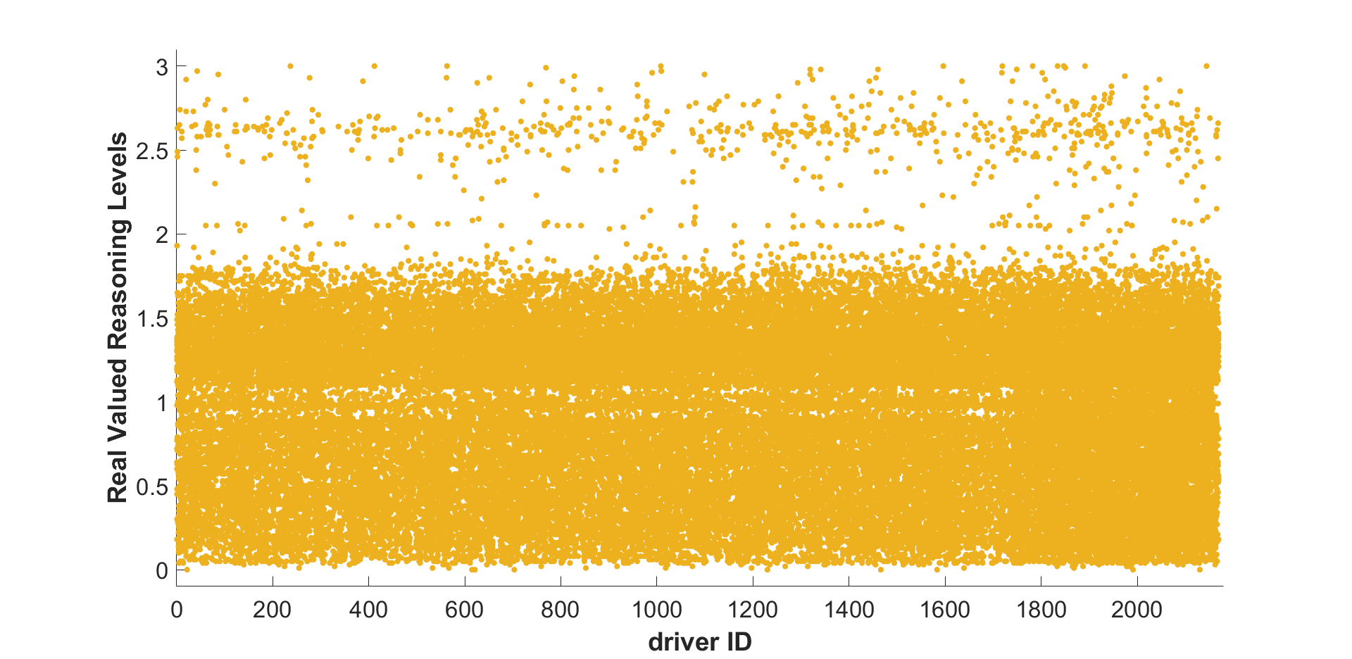
What is more interesting to observe is the distribution of levels among real drivers. Figure 4 shows how this distribution appears for each driver in the traffic data. Each yellow dot on the figure indicates a certain level (given in the y-axis) assigned for a given state of an individual driver (driver ID is given in the x-axis). It is observed that most of the drivers’ reasoning levels are accumulated between level- $0$ and level- $1.75$ . The significant gap at level- $1.75$ and above indicates that in general human drivers act as if other drivers in the traffic do not have reasoning levels of 1 or above. Curiously, this finding is in harmony with the experimental results reported in [53], [54] and pointed out in [44], where it is found that in the Beauty Contest game, for example, with $\rho=2/3$ or $\rho=1/2$ , humans behave mainly as level 1 and 2 and rarely level-3. In [54], unlike in this work, a simple level-0 strategy, corresponding to the bet of 50, which is the average number, is used. On the other hand, in this work, level-0 reasoning corresponds to a strategy which is a driving style determining actions in many different scenarios, and consequently, it is a dramatically more complex strategy in comparison to [54]. This explains the low frequency of level-0 players in [54].

Another demonstration of level distribution of real drivers is given in Figure 5. The y-axis shows the driver ID whereas the x-axis indicates the intervals of real-valued reasoning levels. In particular, intervals are quantized uniformly in which each interval has a size of 0.2 such as $[0.9,1.1)$ except the first and last interval, which are given as $[0,0.3)$ and $[2.7,3.0]$ . The color-bar on the right shows the percentage of the states in the corresponding interval. The figure demonstrates that human drivers mostly have reasoning levels in the interval $[1.1,1.5)$ , followed by the interval $[0.0,0.9)$ . As suggested by the previous result, reasonings in higher levels are not common.

7 Summary

In this study, we proposed a refinement to level- $k$ game theoretical reasoning concept where we introduced continuous levels through multi-output Gaussian Processes. This fills a gap in the literature of level- $k$ game theoretical reasoning concept, which limits us to a few discrete levels for modeling human driver behavior. We also put forward a best response theorem to show that the hierarchical relation is still well defined when the real-valued level policies are linear combinations of integer-valued ones. The proposed approach is validated on real traffic data. Employing US101 driving data, and using Kolmogorov-Smirnov goodness of fit test, it is shown that most of the drivers embrace a behavioral reasoning that is consistent with previous studies.

References

[1] E. Yurtsever, J. Lambert, A. Carballo, and K. Takeda, “A survey of autonomous driving: Common practices and emerging technologies,” IEEE Access, vol. 8, pp. 58443–58469, 2020.
[2] G. Sand and P. Terwiesch, “Closing the loops: An industrial perspective on the present and future impact of control,” European Journal of Control, vol. 19, no. 5, pp. 341–350, 2013.
[3] A. Carvalho, S. Lefévre, G. Schildbach, J. Kong, and F. Borrelli, “Automated driving: The role of forecasts and uncertainty—a control perspective,” European Journal of Control, vol. 24, pp. 14–32, 2015.
[4] N. Kalra and S. M. Paddock, “Driving to safety: How many miles of driving would it take to demonstrate autonomous vehicle reliability?,” Transportation Research Part A: Policy and Practice, vol. 94, pp. 182–193, 2016.
[5] Y. Yildiz, A. Agogino, and G. Brat, “Predicting pilot behavior in medium-scale scenarios using game theory and reinforcement learning,” Journal of Guidance, Control, and Dynamics, vol. 37, no. 4, pp. 1335–1343, 2014.
[6] N. Musavi, D. Onural, K. Gunes, and Y. Yildiz, “Unmanned aircraft systems airspace integration: A game theoretical framework for concept evaluations,” Journal of Guidance, Control, and Dynamics, vol. 40, no. 1, pp. 96–109, 2017.
[7] B. M. Albaba and Y. Yildiz, “Modeling cyber-physical human systems via an interplay between reinforcement learning and game theory,” Annual Reviews in Control, vol. 48, pp. 1–21, 2019.
[8] B. M. Albaba, N. Musavi, and Y. Yildiz, “A 3d game theoretical framework for the evaluation of unmanned aircraft systems airspace integration concepts,” Transportation Research Part C: Emerging Technologies, vol. 133, 2021.
[9] N. Li, D. W. Oyler, M. Zhang, Y. Yildiz, I. Kolmanovsky, and A. R. Girard, “Game theoretic modeling of driver and vehicle interactions for verification and validation of autonomous vehicle control systems,” IEEE Transactions on control systems technology, vol. 26, no. 5, pp. 1782–1797, 2017.
[10] C. Koprulu and Y. Yildiz, “Act to reason: A dynamic game theoretical driving model for highway merging applications,” IEEE Conference on Control Technology and Applications, accepted for publication, 2021.
[11] S. Karimi and A. Vahidi, “Receding horizon motion planning for automated lane change and merge using monte carlo tree search and level-k game theory,” in 2020 American Control Conference (ACC), pp. 1223–1228, IEEE, 2020.
[12] M. Zhang, N. Li, A. Girard, and I. Kolmanovsky, “A finite state machine based automated driving controller and its stochastic optimization,” in Dynamic Systems and Control Conference, vol. 58288, p. V002T07A002, American Society of Mechanical Engineers, 2017.
[13] M. Jain, K. Brown, and A. K. Sadek, “Multi-fidelity recursive behavior prediction,” arXiv preprint arXiv:1901.01831, 2018.
[14] C. F. Camerer, T.-H. Ho, and J.-K. Chong, “A cognitive hierarchy model of games,” The Quarterly Journal of Economics, vol. 119, no. 3, pp. 861–898, 2004.
[15] D. O. Stahl and P. W. Wilson, “On players′ models of other players: Theory and experimental evidence,” Games and Economic Behavior, vol. 10, no. 1, pp. 218–254, 1995.
[16] V. P. Crawford and N. Iriberri, “Level-k auctions: Can a nonequilibrium model of strategic thinking explain the winner’s curse and overbidding in private-value auctions?,” Econometrica, vol. 75, no. 6, pp. 1721–1770, 2007.
[17] M. A. Costa-Gomes, V. P. Crawford, and N. Iriberri, “Comparing models of strategic thinking in van huyck, battalio, and beil’s coordination games,” Journal of the European Economic Association, vol. 7, no. 2-3, pp. 365–376, 2009.
[18] B. M. Albaba and Y. Yildiz, “Driver modeling through deep reinforcement learning and behavioral game theory,” IEEE Transactions on Control Systems Technology, in press, 2021. Available: https://ieeexplore.ieee.org/abstract/document/9424171.
[19] K. Brown, K. Driggs-Campbell, and M. J. Kochenderfer, “Modeling and prediction of human driver behavior: A survey,” arXiv preprint arXiv:2006.08832, 2020.
[20] K. Gillmeier, F. Diederichs, and D. Spath, “Prediction of ego vehicle trajectories based on driver intention and environmental context,” in 2019 IEEE Intelligent Vehicles Symposium (IV), pp. 963–968, IEEE, 2019.
[21] P. Angkititrakul, T. Ryuta, T. Wakita, K. Takeda, C. Miyajima, and T. Suzuki, “Evaluation of driver-behavior models in real-world car-following task,” in 2009 IEEE International Conference on Vehicular Electronics and Safety (ICVES), pp. 113–118, IEEE, 2009.
[22] D. Åsljung, M. Westlund, and J. Fredriksson, “A probabilistic framework for collision probability estimation and an analysis of the discretization precision,” in 2019 IEEE Intelligent Vehicles Symposium (IV), pp. 52–57, IEEE, 2019.
[23] S. Lefèvre, C. Laugier, and J. Ibañez-Guzmàn, “Intention-aware risk estimation for general traffic situations, and application to intersection safety,” 2013.
[24] J. Han, D. Karbowski, N. Kim, and A. Rousseau, “Human driver modeling based on analytical optimal solutions: Stopping behaviors at the intersections,” in Dynamic Systems and Control Conference, vol. 59162, p. V003T18A010, American Society of Mechanical Engineers, 2019.
[25] D. Sadigh, S. Sastry, S. A. Seshia, and A. D. Dragan, “Planning for autonomous cars that leverage effects on human actions.,” in Robotics: Science and Systems, vol. 2, Ann Arbor, MI, USA, 2016.
[26] L. Sun, W. Zhan, and M. Tomizuka, “Probabilistic prediction of interactive driving behavior via hierarchical inverse reinforcement learning,” in 2018 21st International Conference on Intelligent Transportation Systems (ITSC), pp. 2111–2117, IEEE, 2018.
[27] A. Armand, D. Filliat, and J. Ibanez-Guzman, “Modelling stop intersection approaches using gaussian processes,” in 16th International IEEE Conference on Intelligent Transportation Systems (ITSC 2013), pp. 1650–1655, IEEE, 2013.
[28] Q. Tran and J. Firl, “Online maneuver recognition and multimodal trajectory prediction for intersection assistance using non-parametric regression,” in 2014 IEEE Intelligent Vehicles Symposium Proceedings, pp. 918–923, IEEE, 2014.
[29] M. Krüger, A. S. Novo, T. Nattermann, and T. Bertram, “Probabilistic lane change prediction using gaussian process neural networks,” in 2019 IEEE Intelligent Transportation Systems Conference (ITSC), pp. 3651–3656, IEEE, 2019.
[30] Y. Guo, V. V. Kalidindi, M. Arief, W. Wang, J. Zhu, H. Peng, and D. Zhao, “Modeling multi-vehicle interaction scenarios using gaussian random field,” in 2019 IEEE Intelligent Transportation Systems Conference (ITSC), pp. 3974–3980, IEEE, 2019.
[31] L. Schester and L. E. Ortiz, “Longitudinal position control for highway on-ramp merging: A multi-agent approach to automated driving,” in 2019 IEEE Intelligent Transportation Systems Conference (ITSC), pp. 3461–3468, IEEE, 2019.
[32] K. Kang and H. A. Rakha, “Modeling driver merging behavior: a repeated game theoretical approach,” Transportation research record, vol. 2672, no. 20, pp. 144–153, 2018.
[33] Z. Yan, J. Wang, and Y. Zhang, “A game-theoretical approach to driving decision making in highway scenarios,” in 2018 IEEE Intelligent Vehicles Symposium (IV), pp. 1221–1226, IEEE, 2018.
[34] A. Talebpour, H. S. Mahmassani, and S. H. Hamdar, “Modeling lane-changing behavior in a connected environment: A game theory approach,” Transportation Research Part C: Emerging Technologies, vol. 59, pp. 216–232, 2015.
[35] X. Wang, R. Jiang, L. Li, Y. Lin, X. Zheng, and F.-Y. Wang, “Capturing car-following behaviors by deep learning,” IEEE Transactions on Intelligent Transportation Systems, vol. 19, no. 3, pp. 910–920, 2017.
[36] P. Gebert, A. Roitberg, M. Haurilet, and R. Stiefelhagen, “End-to-end prediction of driver intention using 3d convolutional neural networks,” in 2019 IEEE Intelligent Vehicles Symposium (IV), pp. 969–974, IEEE, 2019.
[37] A. Kuefler, J. Morton, T. Wheeler, and M. Kochenderfer, “Imitating driver behavior with generative adversarial networks,” in 2017 IEEE Intelligent Vehicles Symposium (IV), pp. 204–211, IEEE, 2017.
[38] J. Ho and S. Ermon, “Generative adversarial imitation learning,” in Advances in neural information processing systems, pp. 4565–4573, 2016.
[39] N. Musavi, K. B. Tekelioğlu, Y. Yildiz, K. Gunes, and D. Onural, “A game theoretical modeling and simulation framework for the integration of unmanned aircraft systems in to the national airspace,” in AIAA Infotech@ Aerospace, p. 1001, 2016.
[40] M. Albaba, Y. Yildiz, N. Li, I. Kolmanovsky, and A. Girard, “Stochastic driver modeling and validation with traffic data,” in 2019 American Control Conference (ACC), pp. 4198–4203, IEEE, 2019.
[41] R. Tian, S. Li, N. Li, I. Kolmanovsky, A. Girard, and Y. Yildiz, “Adaptive game-theoretic decision making for autonomous vehicle control at roundabouts,” in 2018 IEEE Conference on Decision and Control (CDC), pp. 321–326, IEEE, 2018.
[42] N. Li, Y. Yao, I. Kolmanovsky, E. Atkins, and A. Girard, “Game-theoretic modeling of multi-vehicle interactions at uncontrolled intersections,” arXiv preprint arXiv:1904.05423, 2019.
[43] M. Garzón and A. Spalanzani, “Game theoretic decision making for autonomous vehicles’ merge manoeuvre in high traffic scenarios,” in 2019 IEEE Intelligent Transportation Systems Conference (ITSC), pp. 3448–3453, IEEE, 2019.
[44] R. Lee and D. Wolpert, “Game theoretic modeling of pilot behavior during mid-air encounters,” in Decision Making with Imperfect Decision Makers, pp. 75–111, Springer, 2012.
[45] V. Mnih, K. Kavukcuoglu, D. Silver, A. A. Rusu, J. Veness, M. G. Bellemare, A. Graves, M. Riedmiller, A. K. Fidjeland, G. Ostrovski, et al., “Human-level control through deep reinforcement learning,” Nature, vol. 518, no. 7540, pp. 529–533, 2015.
[46] M. A. Alvarez, L. Rosasco, and N. D. Lawrence, “Kernels for vector-valued functions: A review,” arXiv preprint arXiv:1106.6251, 2011.
[47] M. Salzmann and R. Urtasun, “Implicitly constrained gaussian process regression for monocular non-rigid pose estimation,” Advances in Neural Information Processing Systems, vol. 23, pp. 2065–2073, 2010.
[48] U.F.H. Administration,, “Us101 dataset.” https://www.fhwa.dot.gov/publications/research/operations/07030. Accessed: 2010-09-30.
[49] W. J. Conover, “A kolmogorov goodness-of-fit test for discontinuous distributions,” Journal of the American Statistical Association, vol. 67, no. 339, pp. 591–596, 1972.
[50] M. L. Stein, Interpolation of Spatial Data: Some Theory for Kriging. Springer Science & Business Media, 1999.
[51] GPy, “GPy: A gaussian process framework in python.” http://github.com/SheffieldML/GPy, since 2012.
[52] S. Kirkpatrick, C. D. Gelatt, and M. P. Vecchi, “Optimization by simulated annealing,” science, vol. 220, no. 4598, pp. 671–680, 1983.
[53] C. F. Camerer, Behavioral game theory: Experiments in strategic interaction. Princeton university press, 2011.
[54] R. Nagel, “Unraveling in guessing games: An experimental study,” The American Economic Review, vol. 85, no. 5, pp. 1313–1326, 1995.

Modeling Human Driver Interactions Using an Infinite Policy Space Through Gaussian Processes

Abstract

1 Introduction

2 Related Work

3 Background

3.1 Level-k Reasoning, Deep Reinforcement Learning and Their Synergistic Employment

3.2 Gaussian Processes

3.2.1 Single Output Gaussian Processes

3.2.2 Multi-output Gaussian Processes

4 Method

4.1 Continuous Hierarchical Modelling

Remark.

Remark.

4.2 Best Response in Real-Valued Reasoning Levels

Definition 1.

Theorem 1.

Proof.

5 Validation with Traffic Data

5.1 Construction of the Gaussian Process

5.2 Comparison of Continuous Game Theoretical Policies and Policies Extracted from Driver Data

Definition 2.

Definition 3.

6 Results and Discussion

7 Summary

References

Modeling Human Driver Interactions
Using an Infinite Policy Space Through Gaussian Processes