Efficiently simulating the work distribution of multiple identical bosons with boson sampling

We consider that $N$ identical bosons in a quantum system are driven by a varied external work parameter $\lambda$ from initial time $t=0$ to final time $t=\tau$. The work parameter $\lambda$ could be the position of the quantum piston or the spring coefficient of the harmonic oscillator. Suppose that at initial time $t=0$, the parameter is $\lambda(0)=\lambda_{0}$ and the system is prepared in a thermal state with a heat bath at an inverse temperature $\beta=1/(k_{B}T)$. Here $k_{B}$ is the Boltzmann constant and $T$ is the temperature of the system. After preparing a thermal state, we perform a projective measurement over the energy eigenstates of the system. The probability of bosons initially occupying in the energy eigenstate $|i^{\lambda_{0}}:n_{i}^{\lambda_{0}}\rangle$ is expressed by

Here $Z^{\lambda_{0}}$ is a partition function, which is given by $Z^{\lambda_{0}}=\sum_{i}\text{exp}\big({-\beta n_{i}^{\lambda_{0}}E_{i}^{\lambda_{0}}}\big)$. $E_{i}^{\lambda_{0}}$ is the $i$th eigenenergy at initial time $t=0$, and its corresponding eigenstate is $|i^{\lambda_{0}}\rangle$. $n_{i}^{\lambda_{0}}$ represents the initial occupation number of bosons in the $i$th eigenstate $|i^{\lambda_{0}}\rangle$.

Then the system is detached from the heat bath, and the work parameter of the system is changed from $\lambda(0)=\lambda_{0}$ at initial time $t=0$ to $\lambda(\tau)=\lambda_{\tau}$ at final time $t=\tau$ to perform the work on the system. Finally, we apply the second measurement to project the system into its energy eigenstates again. During the process, the system is evolved under the unitary dynamics and the work distribution of the system can be written as Tasaki 2000; Talkner et al. 2007

Here $E_{f}^{\lambda_{\tau}}$ is the $f$th eigenenergy at final time $t=\tau$, and its corresponding eigenstate is $|f^{\lambda_{\tau}}\rangle$. $n_{f}^{\lambda_{\tau}}$ represents the final occupation number of bosons in the $f$th eigenstate $|f^{\lambda_{\tau}}\rangle$. $P\big(|i^{\lambda_{0}}:n_{i}^{\lambda_{0}}\rangle\rightarrow|f^{\lambda_{\tau}}:n_{f}^{\lambda_{\tau}}\rangle\big)$ is a transition probability from the initial multi-boson eigenstate $|i^{\lambda_{0}}:n_{i}^{\lambda_{0}}\rangle$ to the final multi-boson eigenstate $|f^{\lambda_{\tau}}:n_{f}^{\lambda_{\tau}}\rangle$. The work distribution of multiple particles can be further rewritten as

Here the probability of initial thermal states is described by a vector $P(\mathbf{I})$ and $P(\mathbf{I})=(P(|1^{\lambda_{0}}:n_{1}^{\lambda_{0}}\rangle),P(|2^{\lambda_{0}}:n_{2}^{\lambda_{0}}\rangle),\cdots)$. $\mathbf{I}=(|1^{\lambda_{0}}:n_{1}^{\lambda_{0}}\rangle,|2^{\lambda_{0}}:n_{2}^{\lambda_{0}}\rangle,\cdots)$ is the initial eigenstate vector and its corresponding initial boson number distribution is given by $\mathbf{n_{I}^{\lambda_{0}}}=(n_{1}^{\lambda_{0}},n_{2}^{\lambda_{0}},\cdots)$. $\mathbf{F}=(|1^{\lambda_{\tau}}:n_{1}^{\lambda_{\tau}}\rangle,|2^{\lambda_{\tau}}:n_{2}^{\lambda_{\tau}}\rangle,\cdots)$ is the final eigenstate vector and its corresponding final boson number distribution is given by $\mathbf{n_{F}^{\lambda_{\tau}}}=(n_{1}^{\lambda_{\tau}},n_{2}^{\lambda_{\tau}},\cdots)$. $P(\mathbf{F}|\mathbf{I})$ denotes the transition probability from the initial multi-boson eigenstate vector $\mathbf{I}$ to the final multi-boson eigenstate vector $\mathbf{F}$. From Eq. (3), one can see clearly that the work distribution is mainly determined by two factors. One is the initial thermal distribution probability in Eq. (1), which can be easily calculated on the classical computer. The other is the transition probability $P(\mathbf{F}|\mathbf{I})$ between the multi-boson eigenstates, which is a classically difficult problem to calculate. Due to the interference of multiple identical bosons, the transition probability between multi-boson eigenstates can be constructed from the permanent of the transition amplitude matrix between single-boson eigenstates and it is expressed by Gong et al. 2014; Tichy et al. 2012; Tichy 2014

Here matrix function Per($\Lambda$) represents the permanent of a matrix $\Lambda$. $\Lambda$=$\big(\langle f^{\lambda_{\tau}}|\hat{U}|i^{\lambda_{0}}\rangle\big)$ is a transition amplitude matrix between single-boson eigenstates. $\hat{H}(t)$ is the Hamiltonian of the system, and $\hat{U}$ denotes an evolutionary unitary operator of the system satisfying the time-dependent Schrödinger equation $i\hbar\partial_{t}\hat{U}(t)=\hat{H}(t)\hat{U}(t)$. $\Lambda^{(\mathbf{n_{F}^{\lambda_{\tau}}},\mathbf{n_{I}^{\lambda_{0}}})}$ denotes a sub-matrix of $\Lambda$ by taking $n_{f}^{\lambda_{\tau}}$ ($f=1,2,\cdots$) copies of the $f$th column and $n_{i}^{\lambda_{0}}$ ($i=1,2,\cdots$) copies of the $i$th row of $\Lambda$. Since the total number of bosons is conserved, i.e., $\sum_{i=1}n_{i}^{\lambda_{0}}=\sum_{f=1}n_{f}^{\lambda_{\tau}}=N$, $\Lambda^{(\mathbf{n_{F}^{\lambda_{\tau}}},\mathbf{n_{I}^{\lambda_{0}}})}$ occupies a dimension of $N\times N$.

As shown is Fig. 1, $N$ identical bosons in a one-dimensional quantum piston is an interesting example to understand the work distribution. At $t=0$, the bosons are prepared into a thermal state in a stretchable box of length $\lambda_{0}$ (see Fig. 1a), and their population in the eigenstates is schematically shown in Fig. 1c. Then, the box is stretched to the length $\lambda_{\tau}$ ($\lambda_{\tau}>\lambda_{0}$) at a constant speed $v$ (see Fig. 1b) and at this time the population of bosons in the eigenstates is schematically presented in Fig. 1d. In Appendix A, we provide an explicit expression for constructing the transition amplitude matrix $\Lambda$ between the single-boson eigenstates Quan and Jarzynski 2012; Doescher and Rice 1969. Note that calculating the transition probability between the multi-boson eigenstates in Eq. (4) is a classically difficult problem, because the computational complexity of the permanent of a general complex matrix is #P-hard Valiant 1979; Aaronson 2011. To solve the work distribution problem, in the following text, we would use the boson sampling to simulate the work distribution with multiple identical bosons.

Boson sampling is considered as there are $N$ indistinguishable bosons are scattered into a linear unitary network with $M$ optical modes. We denote the input photon state in the Fock basis as $|\text{{T}}\rangle=|t_{1},t_{2},\cdots,t_{M}\rangle$. Each $t_{i}$ denotes boson occupation-number in the $i$th optical mode and $|\text{{T}}\rangle$ describes $N=\sum_{i=1}^{M}t_{i}$ bosons distribution in each mode. These photons are sent through a linear optical network that is characterized by a unitary transformation $A$. According to the linear mapping relation $a_{i}^{\dagger}\rightarrow\sum_{j=1}^{M}A_{ij}b_{j}^{\dagger}$ between the input mode creation operator $a^{\dagger}$ and the output mode creation operator $b^{\dagger}$ of the network, the probability of getting an output state $|\text{{S}}\rangle=|s_{1},s_{2},\cdots,s_{M}\rangle$ in the Fock basis is mathematically described by Broome et al. 2013; Spring et al. 2013; Tillmann et al. 2013; Crespi et al. 2013,

Remarkably, the probability $P\big(\textbf{S}\,|\,\textbf{T}\big)$ for each of input states and output states is proportional to a permanent of sub-matrix of $A$. Combining Eq. (2), Eq. (4), and Eq. (5), we present a corresponding relationship between the work distribution and boson sampling in Tab. 1. As shown in Tab. 1, one can see that the space of the work distribution with $N$ bosons and $M$-dimensional transition amplitude matrix is isomorphic to the space of boson sampling with $N$ bosons and $M$-dimensional optical network. Therefore, the work distribution can be obtained by sampling from a great quantity of matrix permanents, equivalently to the boson sampling problem.

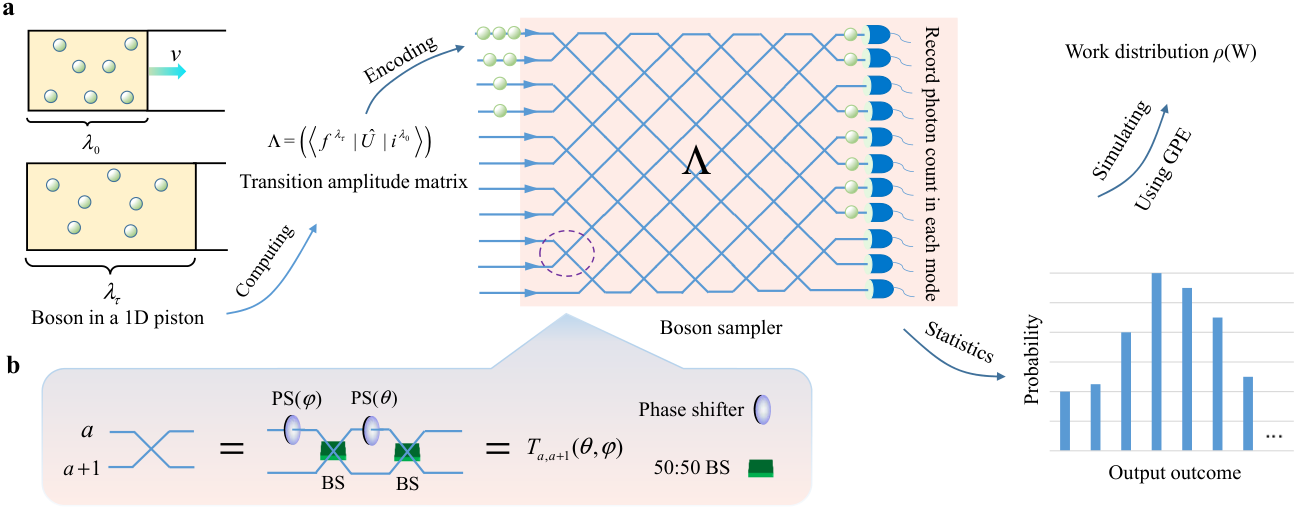
As shown in Fig. 2, we design a schematic setup for simulating the work distribution of multiple identical bosons via boson sampling. We first carefully prepare the input Fock state to simulate the initial thermal state of the multiparticle bosonic system. The input Fock state $|\text{{T}}\rangle_{n}$ in the $n$th optical mode represents the $n$th energy eigenstate of the initial thermal state with the probability $P_{n}$ that can be calculated through the Eq. (1). The similar method to prepare the thermal state has been experimentally demonstrated Sivananda et al. 2020. We then construct the optical network based on the transition amplitude matrix $\Lambda$ between the single-boson eigenstates. The matrix elements $\langle f^{\lambda_{\tau}}|\hat{U}|i^{\lambda_{0}}\rangle$ described in Eq. (20) can be calculated numerically, which depend on the parameters $\lambda_{0},\lambda_{\tau}$, and $v$. The transition amplitude matrix $\Lambda$ is a unitary matrix in principle because the dimension of the matrix $\Lambda$ could be infinite and the matrix $\Lambda$ satisfies the normalization,

However, in reality we have to restrict the dimension of the matrix $\Lambda$ to be finite to encode the matrix into a finite dimensional unitary optical network of boson sampling, which causes the matrix $\Lambda$ to become near-unitary and introduces an encoding error. We can truncate the size of the matrix $\Lambda$ to make it as unitary as possible to reduce the encoding error. We evaluate the error by calculating the unitary fidelity of the matrix $\Lambda$, which is defined as Gilchrist et al. 2005

Here $d$ is the dimension of $\Lambda$ and $I_{d}$ is a $d$-order identity matrix. $\sigma=\Lambda\Lambda^{\prime}$ and $\Lambda^{\prime}$ is the Hermitian conjugate of $\Lambda$. The encoding error $\mathcal{E}$ is described by $\mathcal{E}=1-\mathcal{F}$. We numerically calculate the matrix elements and truncate the size of matrix $\Lambda$ when the encoding error is 0.5% with the fixed parameters $\lambda_{0}=1$, $\lambda_{\tau}=2$ and a varied speed $v$. A relationship between the matrix dimension and the expansion speed $v$ is plotted in Fig. 3a. We also present a relationship between the matrix dimension and the final length of the box in Fig. 3b. As shown in Fig. 3, one can see that the dimension of the matrix $\Lambda$ increases almost linearly with the acceleration of the piston speed $v$ or the final length $\lambda_{\tau}$ of the box. Besides, we note that if the truncated $\Lambda$ matrix as a submatrix is embedded into a unitary matrix Björklund et al. 2019 or increasing the dimension of the truncated $\Lambda$ matrix, the encoding error can be further reduced. In general, the dimension of the optical network will become bigger as the encoding error decreases.

The next step is to encode the transition amplitude matrix $\Lambda$ into a linear optical network. There are mainly two configurations of optical network to realize arbitrary unitary matrix, one is the triangle-shaped network Reck et al. 1994 and the other is the square-shaped network Clements et al. 2016. As shown in Fig. 2a, here we use the square-shaped network to realize the transition amplitude matrix, because the symmetry design of the network is more robust against the photon loss and has minimal optical depth and better stability Clements et al. 2016. As shown in Fig. 2b, the crossing between two optical modes $a$ and $a+1$ in the interferometer consists of two 50:50 beam splitters and two phase shifters, which can be expressed mathematically by a matrix $T_{a,a+1}(\theta,\varphi)$ Clements et al. 2016. $T_{a,a+1}(\theta,\varphi)$ is called an elimination matrix and it is obtained by replacing the entries of an identity matrix with the same size as $\Lambda$ at the $a$th and $(a+1)$th rows and the $a$th and $(a+1)$th columns with

and the rest of the other entries remain unchanged. Based on Gaussian elimination method, the matrix $\Lambda$ can be diagonalized into a diagonal matrix $D$ by multiplying a series of $T_{a,a+1}$ and its inverse matrix $T_{a,a+1}^{-1}$. The matrix $\Lambda$ is realized physically in an optical network by choosing suitable values of parameters $\theta$ and $\varphi$ of $T_{a,a+1}$ and the phase values of diagonal matrix $D$ at each output port. The resource overhead for encoding a $d\times d$ unitary matrix into the optical network requires $d(d-1)$ 50:50 beam splitters and $d^{2}$ phase shifters. In boson sampling system, the phase shifters to realize the diagonal matrix $D$ can be removed as only final photon number is sampled, which will not affect the result but can reduce the resource cost. From Fig. 3, one can see that the total resource cost presents at a polynomial hierarchy with the expansion speed $v$ of the piston or the final length $\lambda_{\tau}$ of the box in terms of the number of required optical elements.

The temperature and the speed play an important role in the piston system during the work process. On one hand, from Eq. (1), one can see that the temperature of the system affects the initial distribution of the bosons. The work distribution for two bosons with different temperature is presented in Fig. 4. As shown in Fig. 4, as the temperature increases, the probability that the bosons populate higher energy levels will increase, which makes the higher energy levels need to be considered. As a result, the dimension of the transition amplitude matrix will become larger, making the calculation of the work distribution more complicated.

On the other hand, the moving speed of the piston is related to the transition probability $P\big(|i^{\lambda_{0}}:n_{i}^{\lambda_{0}}\rangle\rightarrow|f^{\lambda_{\tau}}:n_{f}^{\lambda_{\tau}}\rangle\big)$. In the low speed limit, one can get the result $P\big(|i^{\lambda_{0}}:n_{i}^{\lambda_{0}}\rangle\rightarrow|f^{\lambda_{\tau}}:n_{f}^{\lambda_{\tau}}\rangle\big)\rightarrow\delta_{i,f}$ $(v\rightarrow 0)$ based on the quantum adiabatic theorem. Figure 5a shows approximately the initial energy distribution: the highest peak represents the energy from the beginning to the end of the ground state, the second highest peak corresponds to the energy of the first excited state, etc. As shown in Fig. 5, with the increase of the piston speed, the work distribution for two bosons becomes more complex. This is caused by the higher energy level transition of the bosons when the speed becomes faster.

To understand the work distribution simulated by boson sampling well, as an interesting example, we calculate the work distribution of three bosons in 1D quantum piston in detail. We consider three bosons are trapped in a box with the initial length $\lambda_{0}=1$, the stretching speed $v=0.4$, the final length $\lambda_{\tau}=2$, and the temperature $\beta=0.1$. We numerically calculate the matrix elements of $\Lambda$ based on Eq. (20) and obtain a $5\times 5$ dimensional near-unitary matrix $\Lambda_{5}$ with a unitary fidelity $\mathcal{F}=0.9992$ (see Appendix B). We decompose the matrix $\Lambda_{5}$ into the product of a diagonal matrix $D$ and a series of elimination matrices $T_{a,a+1}$ based on Gaussian elimination method Clements et al. 2016. The result of the decomposition is expressed as

As shown in Fig. 6, the matrix $\Lambda_{5}$ is programmed into an optical network of the boson sampler. The values of phase shifter angles $\theta$ and $\varphi$ in the network are calculated and presented in Tab. 2. The diagonal matrix $D$ can be ignored without affecting the final output probability of photons.

Finally, we calculate the cumulative work distribution by the definition as follows

The result of cumulative work distribution based on Eq. (12) is plotted in the curve of Fig. 7. In real experiments, the noise and error are inevitable. Therefore, we evaluate the effect of the noise on the cumulative work distribution by adding a random noise $\mathcal{N}\in(-0.01,0.01)$ to the angles of the beam splitters. Explicitly, we randomly choose $100$ groups of noise terms and calculate the cumulative work distribution under the noise effects (see error bars in Fig. 7). We find that the ratio between the error bar and the cumulative work distribution curve is $1$% to $2$%.

References

- Jarzynski (1997) C. Jarzynski, Nonequilibrium equality for free energy differences, Phys. Rev. Lett. 78, 2690 (1997).
- Crooks (1999) G. E. Crooks, Entropy production fluctuation theorem and the nonequilibrium work relation for free energy differences, Phys. Rev. E 60, 2721 (1999).
- Hatano and Sasa (2001) T. Hatano and S. I. Sasa, Steady-state thermodynamics of langevin systems, Phys. Rev. Lett. 86, 3463 (2001).
- Kafri and Deffner (2012) D. Kafri and S. Deffner, Holevo’s bound from a general quantum fluctuation theorem, Phys. Rev. A 86, 044302 (2012).
- Deffner and Lutz (2008) S. Deffner and E. Lutz, Nonequilibrium work distribution of a quantum harmonic oscillator, Phys. Rev. E 77, 021128 (2008).
- Quan and Jarzynski (2012) H. T. Quan and C. Jarzynski, Validity of nonequilibrium work relations for the rapidly expanding quantum piston, Phys. Rev. E 85, 031102 (2012).
- Jarzynski et al. (2015) C. Jarzynski, H. T. Quan, and S. Rahav, Quantum-classical correspondence principle for work distributions, Phys. Rev. X 5, 031038 (2015).
- Zhu et al. (2016) L. Zhu, Z. Gong, B. Wu, and H. T. Quan, Quantum-classical correspondence principle for work distributions in a chaotic system, Phys. Rev. E 93, 062108 (2016).
- Łobejko et al. (2017) M. Łobejko, J. Łuczka, and P. Talkner, Work distributions for random sudden quantum quenches, Phys. Rev. E 95, 052137 (2017).
- Batalhão et al. (2014) T. B. Batalhão, A. M. Souza, L. Mazzola, R. Auccaise, R. S. Sarthour, I. S. Oliveira, J. Goold, G. De Chiara, M. Paternostro, and R. M. Serra, Experimental reconstruction of work distribution and study of fluctuation relations in a closed quantum system, Phys. Rev. Lett. 113, 140601 (2014).
- An et al. (2015) S. An, J. N. Zhang, M. Um, D. Lv, Y. Lu, J. Zhang, Z. Q. Yin, H. T. Quan, and K. Kim, Experimental test of the quantum jarzynski equality with a trapped-ion system, Nat. Phys. 11, 193 (2015).
- Sivananda et al. (2020) D. J. Sivananda, N. Roy, P. C. Mahato, and S. S. Banerjee, Exploring the non-equilibrium fluctuation relation for quantum mechanical tunneling of electrons across a modulating barrier, Phys. Rev. Res. 2, 043237 (2020).
- Gong et al. (2014) Z. Gong, S. Deffner, and H. T. Quan, Interference of identical particles and the quantum work distribution, Phys. Rev. E 90, 062121 (2014).
- Wang and Quan (2017) Q. Wang and H. T. Quan, Understanding quantum work in a quantum many-body system, Phys. Rev. E 95, 032113 (2017).
- Wang et al. (2018a) B. Wang, J. Zhang, and H. T. Quan, Work distributions of one-dimensional fermions and bosons with dual contact interactions, Phys. Rev. E 97, 052136 (2018a).
- Goold et al. (2018) J. Goold, F. Plastina, A. Gambassi, and A. Silva, The role of quantum work statistics in many-body physics, in Thermodynamics in the Quantum Regime (Springer, 2018) pp. 317–336.
- Tichy et al. (2012) M. C. Tichy, M. Tiersch, F. Mintert, and A. Buchleitner, Many-particle interference beyond many-boson and many-fermion statistics, New J. Phys. 14, 093015 (2012).
- Tichy (2014) M. C. Tichy, Interference of identical particles from entanglement to boson-sampling, J. Phys. B: At. Mol. Opt. Phys. 47, 103001 (2014).
- Urbina et al. (2016) J. D. Urbina, J. Kuipers, S. Matsumoto, Q. Hummel, and K. Richter, Multiparticle correlations in mesoscopic scattering: Boson sampling, birthday paradox, and Hong-Ou-Mandel profiles, Phys. Rev. Lett. 116, 100401 (2016).
- Valiant (1979) L. G. Valiant, The complexity of computing the permanent, Theor. Comput. Sci. 8, 189 (1979).
- Aaronson (2011) S. Aaronson, A linear-optical proof that the permanent is #P-hard, Proc. R. Soc. A. 467, 3393 (2011).
- Lund et al. (2017) A. P. Lund, M. J. Bremner, and T. C. Ralph, Quantum sampling problems, bosonsampling and quantum supremacy, npj Quantum Inf. 3, 15 (2017).
- Aaronson and Arkhipov (2011) S. Aaronson and A. Arkhipov, The computational complexity of linear optics, in Proceedings of the forty-third annual ACM symposium on Theory of computing (2011) pp. 333–342.
- Gu et al. (2019) X. Gu, M. Erhard, A. Zeilinger, and M. Krenn, Quantum experiments and graphs II: Quantum interference, computation, and state generation, Proc. Natl. Acad. Sci. USA 116, 4147 (2019).
- Arrazola et al. (2021) J. M. Arrazola, V. Bergholm, K. Brádler, T. R. Bromley, M. J. Collins, I. Dhand, A. Fumagalli, T. Gerrits, A. Goussev, L. G. Helt, J. Hundal, T. Isacsson, R. B. Israel, J. Izaac, S. Jahangiri, R. Janik, N. Killoran, S. P. Kumar, J. Lavoie, A. E. Lita, D. H. Mahler, M. Menotti, B. Morrison, S. W. Nam, L. Neuhaus, H. Y. Qi, N. Quesada, A. Repingon, K. K. Sabapathy, M. Schuld, N. Su, J. Swinarton, A. Száva, K. Tan, P. Tan, V. D. Vaidya, Z. Vernon, Z. Zabaneh, and Y. Zhang, Quantum circuits with many photons on a programmable nanophotonic chip, Nature (London) 591, 54 (2021).
- Bao et al. (2023) J. Bao, Z. Fu, T. Pramanik, J. Mao, Y. Chi, Y. Cao, C. Zhai, Y. Mao, T. Dai, X. Chen, X. Jia, L. Zhao, Y. Zheng, B. Tang, Z. Li, J. Luo, W. Wang, Y. Yang, Y. Peng, D. Liu, D. Dai, Q. He, A. L. Muthali, L. K. Oxenløwe, C. Vigliar, S. Paesani, H. Hou, R. Santagati, J. W. Silverstone, A. Laing, M. G. Thompson, J. L. O’Brien, Y. Ding, Q. Gong, and J. Wang, Very-large-scale integrated quantum graph photonics, Nat. Photon. 17, 573–581 (2023).
- Nikolopoulos and Brougham (2016) G. M. Nikolopoulos and T. Brougham, Decision and function problems based on boson sampling, Phys. Rev. A 94, 012315 (2016).
- Nikolopoulos (2019) G. M. Nikolopoulos, Cryptographic one-way function based on boson sampling, Quantum Inf. Process. 18, 259 (2019).
- Huh et al. (2015) J. Huh, G. G. Guerreschi, B. Peropadre, J. R. McClean, and A. Aspuru-Guzik, Boson sampling for molecular vibronic spectra, Nat. Photon. 9, 615 (2015).
- Huh and Yung (2017) J. Huh and M. H. Yung, Vibronic boson sampling: generalized Gaussian boson sampling for molecular vibronic spectra at finite temperature, Sci. Rep. 7, 7462 (2017).
- Shen et al. (2018) Y. Shen, Y. Lu, K. Zhang, J. Zhang, S. Zhang, J. Huh, and K. Kim, Quantum optical emulation of molecular vibronic spectroscopy using a trapped-ion device, Chem. Sci. 9, 836 (2018).
- Wang et al. (2020) C. S. Wang, J. C. Curtis, B. J. Lester, Y. Zhang, Y. Y. Gao, J. Freeze, V. S. Batista, P. H. Vaccaro, I. L. Chuang, L. Frunzio, L. Jiang, S. M. Girvin, and R. J. Schoelkopf, Efficient multiphoton sampling of molecular vibronic spectra on a superconducting bosonic processor, Phys. Rev. X 10, 021060 (2020).
- Banchi et al. (2020) L. Banchi, M. Fingerhuth, T. Babej, C. Ing, and J. M. Arrazola, Molecular docking with Gaussian boson sampling, Sci. Adv. 6, eaax1950 (2020).
- Shi et al. (2022) J. Shi, T. Zhao, Y. Wang, C. Yu, Y. Lu, R. Shi, S. Zhang, and J. Wu, An unbiased quantum random number generator based on boson sampling, arXiv preprint arXiv:2206.02292 (2022).
- Shi et al. (2023) J. Shi, T. Zhao, Y. Wang, Y. Feng, and J. Wu, Chaotic image encryption based on boson sampling, Adv. Quantum Technol. 6, 2200104 (2023).
- Broome et al. (2013) M. A. Broome, A. Fedrizzi, S. Rahimi-Keshari, J. Dove, S. Aaronson, T. C. Ralph, and A. G. White, Photonic boson sampling in a tunable circuit, Science 339, 794 (2013).
- Spring et al. (2013) J. B. Spring, B. J. Metcalf, P. C. Humphreys, W. S. Kolthammer, X. M. Jin, M. Barbieri, A. Datta, N. Thomas-Peter, N. K. Langford, D. Kundys, J. C. Gates, B. J. Smith, P. G. R. Smith, and I. A. Walmsley, Boson sampling on a photonic chip, Science 339, 798 (2013).
- Tillmann et al. (2013) M. Tillmann, B. Dakić, R. Heilmann, S. Nolte, A. Szameit, and P. Walther, Experimental boson sampling, Nat. Photon. 7, 540 (2013).
- Crespi et al. (2013) A. Crespi, R. Osellame, R. Ramponi, D. J. Brod, E. F. Galvao, N. Spagnolo, C. Vitelli, E. Maiorino, P. Mataloni, and F. Sciarrino, Integrated multimode interferometers with arbitrary designs for photonic boson sampling, Nat. Photon. 7, 545 (2013).
- Wang et al. (2017) H. Wang, Y. He, Y. H. Li, Z. E. Su, B. Li, H. L. Huang, X. Ding, M. C. Chen, C. Liu, J. Qin, J. P. Li, Y. M. He, C. Schneider, M. Kamp, C. Z. Peng, S. Höfling, C. Y. Lu, and J. W. Pan, High-efficiency multiphoton boson sampling, Nat. Photon. 11, 361 (2017).
- Wang et al. (2018b) H. Wang, W. Li, X. Jiang, Y. M. He, Y. H. Li, X. Ding, M. C. Chen, J. Qin, C. Z. Peng, C. Schneider, M. Kamp, W. J. Zhang, H. Li, L. X. You, Z. Wang, J. P. Dowling, S. Höfling, C. Y. Lu, and J. W. Pan, Toward scalable boson sampling with photon loss, Phys. Rev. Lett. 120, 230502 (2018b).
- Wang et al. (2019) H. Wang, J. Qin, X. Ding, M. C. Chen, S. Chen, X. You, Y. M. He, X. Jiang, L. You, Z. Wang, C. Schneider, J. J. Renema, S. Höfling, C. Y. Lu, and J. W. Pan, Boson sampling with 20 input photons and a 60-mode interferometer in a -dimensional Hilbert space, Phys. Rev. Lett. 123, 250503 (2019).
- Zhong et al. (2020) H. S. Zhong, H. Wang, Y. H. Deng, M. C. Chen, L. C. Peng, Y. H. Luo, J. Qin, D. Wu, X. Ding, Y. Hu, P. Hu, X. Y. Yang, W. J. Zhang, H. Li, Y. Li, X. Jiang, L. Gan, G. Yang, L. You, Z. Wang, L. Li, N. L. Liu, C. Y. Lu, and J. W. Pan, Quantum computational advantage using photons, Science 370, 1460 (2020).
- Zhong et al. (2021) H. S. Zhong, Y. H. Deng, J. Qin, H. Wang, M. C. Chen, L. C. Peng, Y. H. Luo, D. Wu, S. Q. Gong, H. Su, Y. Hu, P. Hu, X. Y. Yang, W. J. Zhang, H. Li, Y. Li, X. Jiang, L. Gan, G. Yang, L. You, Z. Wang, L. Li, N. L. Liu, J. J. Renema, C. Y. Lu, and J. W. Pan, Phase-programmable Gaussian boson sampling using stimulated squeezed light, Phys. Rev. Lett. 127, 180502 (2021).
- Lau and James (2012) H. K. Lau and D. F. V. James, Proposal for a scalable universal bosonic simulator using individually trapped ions, Phys. Rev. A 85, 062329 (2012).
- Shen et al. (2014) C. Shen, Z. Zhang, and L. M. Duan, Scalable implementation of boson sampling with trapped ions, Phys. Rev. Lett. 112, 050504 (2014).
- Oh et al. (2022) C. Oh, Y. Lim, Y. Wong, B. Fefferman, and L. Jiang, Quantum-inspired classical algorithm for molecular vibronic spectra, arXiv preprint arXiv:2202.01861 (2022).
- Tasaki (2000) H. Tasaki, Jarzynski relations for quantum systems and some applications, arXiv preprint cond-mat/0009244 (2000).
- Talkner et al. (2007) P. Talkner, E. Lutz, and P. Hänggi, Fluctuation theorems: Work is not an observable, Phys. Rev. E 75, 050102(R) (2007).
- Doescher and Rice (1969) S. W. Doescher and M. H. Rice, Infinite square-well potential with a moving wall, Am. J. Phys. 37, 1246 (1969).
- Gilchrist et al. (2005) A. Gilchrist, N. K. Langford, and M. A. Nielsen, Distance measures to compare real and ideal quantum processes, Phys. Rev. A 71, 062310 (2005).
- Björklund et al. (2019) A. Björklund, B. Gupt, and N. Quesada, A faster hafnian formula for complex matrices and its benchmarking on the Titan supercomputer, J. Exp. Algor. 24, 11 (2019).
- Reck et al. (1994) M. Reck, A. Zeilinger, H. J. Bernstein, and P. Bertani, Experimental realization of any discrete unitary operator, Phys. Rev. Lett. 73, 58 (1994).
- Clements et al. (2016) W. R. Clements, P. C. Humphreys, B. J. Metcalf, W. S. Kolthammer, and I. A. Walmsley, Optimal design for universal multiport interferometers, Optica 3, 1460 (2016).