A first taste of nonlinear beam dynamics

A schematic of the bunch compressor that we shall use in this example is shown in Fig. 3 (top), and consists of an RF cavity followed by a chicane constructed from four dipoles. The RF cavity is designed to “chirp” the bunch, i.e. to provide a change in energy deviation as a function of longitudinal position $z$ within the bunch ($z>0$ at the head of the bunch). The accelerating field in the cavity varies with time. Suppose that a particle in the centre of the bunch arrives at the cavity at a time such that the average accelerating field that it sees in the cavity is zero: the energy of this particle will be unchanged. However, particles ahead or behind this particle will see a non-zero field (on average) and will then either gain or lose energy. The energy change $\Delta E$ of a particular particle will depend on the distance by which it is either ahead or behind the centre of the bunch, the RF voltage and frequency of the cavity:

$$\Delta E=-eV\sin(kz).$$

(20)

Here, $V$ is the maximum voltage across the cavity (taking into account the time of flight of a particle through the cavity), $k=\omega/c$ (where $\omega$ is the RF angular frequency and $c$ is the speed of light), and $z$ is the distance of the particle from the centre of the bunch. Note that we use the convention that $z$ is positive for a particle that is ahead of the centre of the bunch. In that case, the minus sign in Eq. (20) means that for a bunch of particles moving through the bunch compressor, the RF cavity reduces the energy of particles at the head of the bunch, and increases the energy of particles in the tail (see Fig. 3, bottom).

For convenience, we define the longitudinal phase space variables as $z$ (the co-ordinate) and $\delta$, the energy deviation. The energy deviation $\delta$ of a particle with energy $E$ is defined as:

$$\delta=\frac{E-E_{0}}{E_{0}},$$

(21)

where $E_{0}$ is the reference energy for the system (corresponding to the energy of a particle with total momentum $P_{0}$, the reference momentum). If the reference momentum is chosen so that it is close to the “average” momentum of particles in the beam, then $\delta$ should be a small number (i.e. $|\delta|\ll 1$) for all particles: this has some advantages when expressing nonlinear transfer maps in terms of power series of the dynamical variables. In terms of the variables $z$ and $\delta$, the transfer map for the RF cavity in the bunch compressor is:

	$\displaystyle z_{1}$	$\displaystyle=$	$\displaystyle z_{0},$		(22)
	$\displaystyle\delta_{1}$	$\displaystyle=$	$\displaystyle\delta_{0}-\frac{eV}{E_{0}}\sin(kz_{0}).$		(23)

Now consider the dynamics in the sequence of four dipoles following the RF cavity: in the example we are considering here, the dipoles form a chicane, so that for a particle with the reference momentum, the trajectory after the exit of the chicane is colinear with the trajectory at the entrance of the chicane. Neglecting synchrotron radiation, the chicane does not change the energy of the particles. However, the path length $L$ depends on the energy of the particle. If we assume that the bending angle in each dipole is small, $\theta\ll 1$, then from Fig. 4 we find that:

$$L=\frac{2L_{1}}{\cos(\theta)}+L_{2}.$$

(24)

The bending angle is a function of the energy of the particle:

$$\theta(\delta)=\frac{\theta_{0}}{1+\delta}.$$

(25)

Assuming that the beam is ultrarelativistic (so that we can neglect differences in the speed of particles arising from differences in energy) the change in the co-ordinate $z$ of a particle after passing through the chicane is the difference between the nominal path length, and the length of the path actually taken by the particle. Hence, the transfer map for the chicane can be written:

	$\displaystyle z_{2}$	$\displaystyle=$	$\displaystyle z_{1}+2L_{1}\left(\frac{1}{\cos(\theta_{0})}-\frac{1}{\cos(\theta(\delta_{1}))}\right),$		(26)
	$\displaystyle\delta_{2}$	$\displaystyle=$	$\displaystyle\delta_{1},$		(27)

where $\theta_{0}$ is the nominal bending angle of each dipole in the chicane, and $\theta(\delta)$ is given by (25).

We can now write down the complete transfer map for the bunch compressor by substituting $z_{1}$ and $\delta_{1}$ from Eqs. (22) and (23) into Eqs. (26) and (27). Expanding the resulting expressions in terms of the dynamical variables provides the transfer map in the form of a power series. Using the standard notation, we write:

	$\displaystyle z_{2}$	$\displaystyle=$	$\displaystyle R_{55}z_{0}+R_{56}\delta_{0}+T_{555}z_{0}^{2}+T_{556}z_{0}\delta_{0}+T_{566}\delta_{0}^{2}+\ldots$		(28)
	$\displaystyle\delta_{2}$	$\displaystyle=$	$\displaystyle R_{65}z_{0}+R_{66}\delta_{0}+T_{655}z_{0}^{2}+T_{656}z_{0}\delta_{0}+T_{666}\delta_{0}^{2}+\ldots$		(29)

The procedure that we have described provides expressions for the coefficients in terms of the bunch compressor parameters. In particular, we find for the coefficients of the linear terms:

	$\displaystyle R_{55}$	$\displaystyle=$	$\displaystyle 1-\frac{eV}{E_{0}}kL_{1}\frac{\theta_{0}\sin(2\theta_{0})}{\cos^{3}(\theta_{0})},$		(30)
	$\displaystyle R_{56}$	$\displaystyle=$	$\displaystyle L_{1}\frac{\theta_{0}\sin(2\theta_{0})}{\cos^{3}(\theta_{0})},$		(31)
	$\displaystyle R_{65}$	$\displaystyle=$	$\displaystyle-\frac{eV}{E_{0}}k,$		(32)
	$\displaystyle R_{66}$	$\displaystyle=$	$\displaystyle 1,$		(33)

The coefficients of the second-order terms are given by:

	$\displaystyle T_{555}$	$\displaystyle=$	$\displaystyle\left(\frac{eV}{E_{0}}k\right)^{2}L_{1}\frac{\theta_{0}(\cos(\theta_{0})-3)-2\sin(2\theta_{0})}{2\cos^{3}(\theta_{0})},$		(34)
	$\displaystyle T_{556}$	$\displaystyle=$	$\displaystyle-\frac{eV}{E_{0}}kL_{1}\frac{\theta_{0}(\cos(\theta_{0})-3)-2\sin(2\theta_{0})}{\cos^{3}(\theta_{0})},$		(35)
	$\displaystyle T_{566}$	$\displaystyle=$	$\displaystyle L_{1}\frac{\theta_{0}(\cos(\theta_{0})-3)-2\sin(2\theta_{0})}{2\cos^{3}(\theta_{0})},$		(36)
	$\displaystyle T_{655}$	$\displaystyle=$	$\displaystyle T_{656}=T_{666}=0.$		(37)

Having constructed the transfer map, the next step is to determine appropriate values for the parameters of the main components, based on consideration of the linear dynamics. The first consideration is the compression factor that the bunch compressor should achieve. This can be written in terms of the mean square values of the initial and final longitudinal co-ordinates:

$$\frac{\langle z_{2}^{2}\rangle}{\langle z_{0}^{2}\rangle}=\frac{1}{b^{2}},$$

(38)

where the brackets $\langle\cdot\rangle$ indicate an average over all particles in the bunch, and $b$ is the required compression factor. If we assume that the beam at the entrance to the bunch compressor has no initial chirp, so that $\langle z_{0}\delta_{0}\rangle=0$, then taking only the linear terms from Eq. (28) gives:

$$\langle z_{2}^{2}\rangle=R_{55}^{2}\langle z_{0}^{2}\rangle+R_{56}^{2}\langle\delta_{0}^{2}\rangle=\frac{\langle z_{0}^{2}\rangle}{b^{2}}.$$

(39)

Generally, the beam exiting the bunch compressor should have no energy chirp, so that $\langle z_{2}\delta_{2}\rangle=0$. Using Eqs. (28) and (29) and again keeping only linear terms gives:

$$\langle z_{2}\delta_{2}\rangle=R_{55}R_{65}\langle z_{0}^{2}\rangle+R_{56}\langle\delta_{0}^{2}\rangle=0.$$

(40)

Note that we have used the fact that $R_{66}=1$. A third (and final) constraint comes from the fact that the linear transfer map must be symplectic: this means that the transfer matrix (with elements $R_{ij}$) must have unit determinant:

$$R_{55}-R_{56}R_{65}=1.$$

(41)

With given initial bunch length, energy spread, and specified compression factor, Eqs. (39), (40) and (41) can be solved to give values for $R_{55}$, $R_{56}$ and $R_{65}$. The result is:

	$\displaystyle R_{55}$	$\displaystyle=$	$\displaystyle\frac{1}{b^{2}},$		(42)
	$\displaystyle R_{56}$	$\displaystyle=$	$\displaystyle\pm\frac{\sqrt{b^{2}-1}}{b^{2}}\sqrt{\frac{\langle z_{0}^{2}\rangle}{\langle\delta_{0}^{2}\rangle}},$		(43)
	$\displaystyle R_{65}$	$\displaystyle=$	$\displaystyle\mp\sqrt{b^{2}-1}\sqrt{\frac{\langle\delta_{0}^{2}\rangle}{\langle z_{0}^{2}\rangle}}.$		(44)

As an example, let us consider the parameters for the bunch compressors in the International Linear Collider, given in Table 1. With the given initial bunch length and energy spread, and the specified final bunch length (and also since $R_{56}$ must be positive in this case), we find that:

	$\displaystyle R_{55}$	$\displaystyle=$	$\displaystyle 0.0025,$		(45)
	$\displaystyle R_{56}$	$\displaystyle=$	$\displaystyle 0.19975\,\textrm{m},$		(46)
	$\displaystyle R_{65}$	$\displaystyle=$	$\displaystyle-4.9937\,\textrm{m}^{-1}.$		(47)

Using these values, we can illustrate the effect of the linearised bunch compressor map on phase space. For clarity and convenience, we use an artificial “window frame” distribution: see Fig. 5. Particles are initially distributed along lines in phase space corresponding to one standard deviation of the nominal distribution. We see that after passing through the bunch compressor, and applying only the linear terms in the transfer map, the rms bunch length is reduced by a factor of 20 as required. The rms energy spread is increased by the same factor, but this is unavoidable, because the transfer map is symplectic; this means that phase space areas are conserved under the transformation, i.e. the longitudinal emittance is conserved (as required by Liouville’s theorem).

Based on the values for the coefficients in the transfer map given in (45), (46) and (47) we can select appropriate values for the parameters of the main components in the bunch compressor. These will also be determined by technical considerations and constraints from the overall design of the facility. Such considerations are beyond the scope of this discussion; but it is found that the parameters given in Table 2 are suitable for the case of the International Linear Collider.

Using the values of the parameters given in Table 2, we can move on to the next step in the design process, which is to evaluate the impact of nonlinear effects. As before, we illustrate the effect of the bunch compressor map on phase space using a “window frame” distribution; this time, however, we can apply the full transfer map expressed in Eqs. (22), (23), (26) and (27). The results are shown in Fig. 6. Although the bunch length has been reduced, there is significant distortion of the distribution: the rms bunch length will be significantly longer than the specification requires. To reduce the distortion, we first need to understand where it comes from, which means looking at the map more closely. Consider a particle entering the bunch compressor with initial energy deviation $\delta_{0}=0$. From the shape of the final phase space²² 2 Note that points along lines of constant energy deviation in the initial phase space are coloured blue: because of the rotation of phase space, the $\delta$ axis in the final phase space plot corresponds (approximately) to the $z$ axis in the initial phase space plot., we see that the final co-ordinate $z_{2}$ varies quadratically with the initial $z_{0}$:

$$z_{2}\propto z_{0}^{2}.$$

(48)

This suggests that the distortion is dominated by the term in the transfer map with coefficient $T_{555}$. To eliminate the distortion, we see from (34) that we would need to choose a bending angle $\theta_{0}$ in the chicane that satisfies:

$$\theta_{0}(\cos(\theta_{0})-3)-2\sin(\theta_{0})=0.$$

(49)

Unfortunately, the only solution to this equation is $\theta_{0}=0$, which would eliminate the chicane altogether, and is incompatible with the linear part of the transfer map. To address the problem of the phase space distortion caused by the nonlinearities, we need to introduce an additional degree of freedom.

Understanding the physical origin of the damaging nonlinearity will help us to identify a possible solution. Since the RF cavity has no effect on the longitudinal co-ordinate, the $T_{555}$ term in the transfer map must come from the chicane: this is confirmed by our observation above, that $T_{555}=0$ if $\theta_{0}=0$, i.e. if we eliminate the chicane altogether. The physical cause of the nonlinear distortion is the second-order dependence of the change in longitudinal co-ordinate on the energy deviation for a particle passing through a dipole. Unfortunately, this effect is intrinsic to dipole magnets, and cannot be corrected within the magnet itself. However, we can compensate for it if we introduce a second-order dependence of the energy deviation on the longitudinal co-ordinate before the bunch enters the chicane.

To see how this works, suppose that we write the transformation of the energy deviation in the first part of the bunch compressor as follows:

$$\delta_{1}=R_{65}^{(1)}z_{0}+T_{655}^{(1)}z_{0}^{2}.$$

(50)

We use the superscript on $R_{ij}^{(1)}$ and $T_{ijk}^{(1)}$ to indicate that the coefficient is for the map for only the first part of the bunch compressor. Then, we write the transformation for the longitudinal co-ordinate in the second part of the bunch compressor:

$$z_{2}=R_{56}^{(2)}\delta_{1}+T_{566}^{(2)}\delta_{1}^{2}.$$

(51)

Substituting $\delta_{1}$ from (50) into (51), and keeping terms only up to second order, we find:

$$z_{2}=R_{56}^{(2)}R_{65}^{(1)}z_{0}+R_{56}^{(2)}T_{655}^{(1)}z_{0}^{2}+T_{566}^{(2)}\left(R_{65}^{(1)}\right)^{2}z_{0}^{2}.$$

(52)

In the transfer map we have used so far for the RF cavity in the bunch compressor, $T_{655}^{(1)}=0$: there is then a second-order dependence of $z_{2}$ on $z_{0}$, with coefficient $T_{566}^{(2)}\left(R_{65}^{(1)}\right)^{2}$. To eliminate this dependence, we need to modify the transformation in the RF cavity so that:

$$T_{555}=R_{56}^{(2)}T_{655}^{(1)}+T_{566}^{(2)}\left(R_{65}^{(1)}\right)^{2}=0.$$

(53)

To achieve this, we simply need to change the phase of the RF cavity, so that a particle at the centre of the bunch sees a non-zero accelerating (or decelerating) field:

$$\delta_{1a}=\delta_{0}-\frac{eV}{E_{0}}\sin(kz_{0}+\phi_{0}).$$

(54)

Although this will introduce the terms that we need in the map to correct the nonlinear distortion, it also means that there is an overall change in the bunch energy. The overall change in energy is inconvenient for the description of the dynamics in the chicane: in order to maintain good accuracy in the power series representation of the transfer map, it is desirable for particles in the bunch to be described by small values of the energy deviation, with mean of zero. To ensure that this is the case, we change the reference energy from $E_{0}$ to $E_{0}-eV\sin(\phi_{0})$. This change in reference energy will restore the mean energy deviation of the bunch to zero; but we also need to take into account, from Eq. (21), that when we change the reference energy from $E_{0}$ to a new value $E_{0}^{\prime}$, the energy deviation changes from $\delta$ to $\delta^{\prime}$:

$$\delta^{\prime}=\left(\delta-\frac{\Delta E_{0}}{E_{0}}\right)\frac{E_{0}}{E_{0}^{\prime}},$$

(55)

where $\Delta E_{0}=E_{0}^{\prime}-E_{0}$. This scaling of the momentum deviation, with no associated change in the longitudinal co-ordinate, is a non-symplectic transformation, and leads to a change in the longitudinal emittance. A similar effect occurs in the transverse degrees of freedom: when associated with acceleration in a linac, it leads to a reduction of the emittances in all three planes, and is known as adiabatic damping. In the present case of the bunch compressor, the result is that the full transformation in the RF cavity is now:

	$\displaystyle z_{1}$	$\displaystyle=$	$\displaystyle z_{0},$		(56)
	$\displaystyle\delta_{1}$	$\displaystyle=$	$\displaystyle\left(\delta_{0}-\frac{eV}{E_{0}}(\sin(kz_{0}+\phi_{0})-\sin(\phi_{0}))\right)\left(1-\frac{eV}{E_{0}}\sin(\phi_{0})\right)^{\!-1}.$		(57)

Expanding to second order in $z_{0}$, this gives:

$$\delta_{1}=\left(1-\frac{eV}{E_{0}}\sin(\phi_{0})\right)^{\!-1}\left(\delta_{0}-\frac{eV}{E_{0}}\cos(\phi_{0})kz_{0}+\frac{eV}{2E_{0}}\sin(\phi_{0})k^{2}z_{0}^{2}+\ldots\right)$$

(58)

Hence:

$$T_{655}^{(1)}=\frac{eV}{2E_{0}}\sin(\phi_{0})k^{2}.$$

(59)

A non-zero value of $\phi_{0}$ leads to a non-zero value for $T_{655}^{(1)}$, and allows us to satisfy the requirement expressed in Eq. (53), to correct the nonlinear distortion arising from $T_{566}^{(2)}$. The other constraints that we need to satisfy are, as before, the specified reduction in bunch length, Eq. (39):

$$R_{55}^{2}+\frac{\langle\delta_{0}^{2}\rangle}{\langle z_{0}^{2}\rangle}R_{56}^{2}=\frac{1}{b^{2}},$$

(60)

and the requirement for zero final energy chirp, Eq. (40):

$$R_{55}R_{65}+\frac{\langle\delta_{0}^{2}\rangle}{\langle z_{0}^{2}\rangle}R_{56}R_{66}=0.$$

(61)

Note that the expressions for the coefficients $R_{ij}$ need to be re-calculated for the case $\phi_{0}\neq 0$: in particular $R_{66}$ is no longer equal to 1. Also, the constraint expressed in Eq. (40) no longer applies, because of the (non-symplectic) rescaling of the reference energy that we have applied following the RF cavity.

We therefore have three constraints, Eq. (53), (60) and (61). Assuming fixed RF frequency and dipole spacing³³ 3 The RF frequency and dipole spacing are fixed at time of machine construction; the RF voltage, RF phase, and dipole bending angle are readily adjusted during operation., we can satisfy the constraints by adjusting the values of the RF voltage $V$, the RF phase $\phi_{0}$, and the dipole bending angle $\theta_{0}$. Given the complicated, nonlinear nature of the constraint equations, the parameter optimisation is best done numerically. Suitable values for the parameters are shown in Table 3.

As before, we illustrate the effect of the bunch compressor on phase space using a “window frame” distribution. But now we use the parameters given in Table 3 to aim to compress the bunch length by a factor 20 while minimising the second-order distortion: the results are shown in Fig. 7. We see that the nonlinear distortion is greatly reduced: the remaining distortion now appears to be dominated by third-order terms, and appears to be small enough that it should not significantly affect the performance of the machine.

The analysis of the bunch compressor presented in this section highlights some important aspects of nonlinear dynamics in accelerators. First, we see that nonlinear effects can limit the performance of an accelerator system. Sometimes the effects are small enough that they can be ignored; however, in many cases, a system designed without taking account of nonlinearities will not achieve the specified performance. Secondly, a careful analysis can lead to an understanding of the nonlinear behaviour of a system, including the origin of the nonlinearities. Based on this analysis, it may be possible to find a means of compensating any adverse effects.

Sextupoles are needed in a storage ring to compensate for the fact that quadrupoles have lower focusing strength for particles of higher energy (see Fig. 8): this is characterised by the chromaticity, which is defined as the change in particle tune in a storage ring with respect to energy deviation. Chromaticity often has undesirable consequences. For example, if particles with sufficiently large energy deviation (by virtue of the natural energy spread of the beam) have betatron tunes close to integer or half-integer values, then the motion of these particles can become unstable, leading to loss of the particles from the storage ring.

A sextupole can be regarded as a quadrupole with focusing strength that increases with horizontal (transverse) distance from the axis of the magnet. If sextupoles are located where there is non-zero dispersion, they can be used to control the chromaticity in a storage ring. The dispersion describes the change in position of the closed orbit with respect to changes in energy deviation: particles with higher energy deviation will then pass through the sextupole further from the axis of the magnet (see Fig. 9), and hence receive additional focusing or defocusing. By adjusting the strength of the sextupole (depending on the size of the dispersion), it is possible to compensate the natural chromaticity arising from the variation of the focal lengths of the quadrupoles with particle energy.

The chromaticity of a storage ring, and hence the strengths of the sextupoles needed to correct the chromaticity, will normally be a function of the phase advance per cell. However, to investigate and illustrate the nonlinear effects of the sextupoles, we shall assume that we keep the strength $k_{2}L$ of the sextupoles in our simple storage ring fixed when we change the phase advance. Although this means that the chromaticity will in general be non-zero, since we shall be looking only at the motion of particles with zero energy deviation, the chromaticity will play no real role. The effects of the sextupoles in this case are sometimes called the geometric effects, to distinguish them from the chromatic effects. The geometric effects of sextupoles can have significant adverse impact on the stability of the motion of particles in a storage ring. Particularly for low-emittance electron storage rings, for example in third-generation synchrotron light sources, it is an important task at the design stage to optimize the chromatic effects of the sextupoles while minimising the geometric effects, in order to achieve a good beam lifetime.

In our simple storage ring, we can assume that the map from one sextupole to the next is linear, and corresponds to a rotation in phase space through an angle equal to the phase advance:

$$\left(\begin{array}[]{c}x\\ p_{x}\end{array}\right)\mapsto\left(\begin{array}[]{cc}\cos(\mu_{x})&\sin(\mu_{x})\\ -\sin(\mu_{x})&\cos(\mu_{x})\\ \end{array}\right)\left(\begin{array}[]{c}x\\ p_{x}\end{array}\right).$$

(62)

Note that we use the symbol $\mapsto$ to mean “transforms to”: this avoids the need to use subscripts to indicate initial and final values of the phase space variables (as in, for example, $x_{0}$ and $x_{1}$). Again to keep things simple, we shall consider only horizontal motion, and assume that the vertical co-ordinate $y=0$.

The change in the horizontal momentum of a particle moving through the sextupole is found by integrating the Lorentz force over the length $L$ of the sextupole:

$$\Delta p_{x}=-\int_{0}^{L}\frac{B_{y}}{B\rho}\,ds.$$

(63)

The sextupole strength $k_{2}$ is defined by:

$$k_{2}=\frac{1}{B\rho}\frac{\partial^{2}B_{y}}{\partial x^{2}},$$

(64)

where $B\rho$ is the beam rigidity. For a pure sextupole field, in the case that the vertical co-ordinate $y=0$, the vertical component of the magnetic field is given by:

$$\frac{B_{y}}{B\rho}=\frac{1}{2}k_{2}x^{2}.$$

(65)

If the sextupole is short (compared to the betatron wavelength), then we can neglect the small change in the co-ordinate $x$ as the particle moves through the sextupole, in which case:

$$\Delta p_{x}\approx-\frac{1}{2}k_{2}Lx^{2}.$$

(66)

Hence, the transfer map for a particle moving through a short sextupole can be represented by a “kick” in the horizontal momentum:

	$\displaystyle x$	$\displaystyle\mapsto$	$\displaystyle x,$		(67)
	$\displaystyle p_{x}$	$\displaystyle\mapsto$	$\displaystyle p_{x}-\frac{1}{2}k_{2}Lx^{2}.$		(68)

To illustrate the effect of the sextupole in our storage ring, let us choose a fixed value $k_{2}L=-600\,\textrm{m}^{-2}$ for the strength of the sextupole, and look at the effects of the maps for different phase advances. As mentioned above, we shall only consider the case that the particles have zero energy deviation. For a given value of the phase advance, we construct a phase space portrait by plotting the values of the dynamical variables after repeated application of the transfer map (equation (62), followed by (67) and (68)) for a range of initial conditions. The phase space portraits for the simple storage ring with a range of phase advances from $0.2\times 2\pi$ to $0.5\times 2\pi$ are shown in Fig. 10.

There are some interesting features in these phase space portraits to which it is worth drawing attention:

• •

  For small amplitudes (small $x$ and $p_{x}$), particles trace out closed loops around the origin: this is what we expect for a purely linear map.

• •

  As the amplitude is increased, “islands” appear in the phase space, with the number of islands related to the phase advance: the phase advance (for the linear map) is often close to $m/p$ where $m$ is an integer and $p$ is the number of islands.

• •

  Sometimes, a larger number of islands appears at larger amplitude.

• •

  Usually, there is a closed curve that divides a region of stable motion from a region of unstable motion. Outside that curve, the amplitude of particles increases without limit as the map is repeatedly applied, i.e. the motion is unstable.

• •

  The area of the stable region depends strongly on the phase advance: for a phase advance close to $2\pi/3$, it appears that the stable region almost vanishes altogether.

• •

  As the phase advance is increased towards $\pi$, the stable area becomes large, and distortions from the linear ellipse become less evident.

An important observation is that the effect of the sextupole in the periodic cell depends strongly on the phase advance across the cell. We can start to understand the significance of the phase advance by considering two special cases: first, the case when the phase advance is equal to an integer times $2\pi$; and second, when the phase advance is equal to a half integer times $2\pi$. In the first case, when the phase advance is an integer, the linear part of the map is just the identity:

	$\displaystyle x$	$\displaystyle\mapsto$	$\displaystyle x,$		(69)
	$\displaystyle p_{x}$	$\displaystyle\mapsto$	$\displaystyle p_{x}.$		(70)

So the combined effect of the linear map and the sextupole kick is:

	$\displaystyle x$	$\displaystyle\mapsto$	$\displaystyle x,$		(71)
	$\displaystyle p_{x}$	$\displaystyle\mapsto$	$\displaystyle p_{x}-\frac{1}{2}k_{2}Lx^{2}.$		(72)

Clearly, for $x\neq 0$, the horizontal momentum will increase without limit. There are no stable regions of phase space, apart from the line $x=0$.

Now consider what happens in the second case, when the phase advance over one cell is a half integer times $2\pi$, so the linear part of the map is just a rotation by $\pi$. If a particle starts at the entrance of a sextupole with $x=x_{0}$ and $p_{x}=p_{x0}$, then at the exit of that sextupole (using the subscript notation to indicate initial and final values of the variables):

	$\displaystyle x_{1}$	$\displaystyle=$	$\displaystyle x_{0},$		(73)
	$\displaystyle p_{x1}$	$\displaystyle=$	$\displaystyle p_{x0}-\frac{1}{2}k_{2}Lx_{0}^{2}.$		(74)

Then, after passing to the entrance of the next sextupole, the phase space variables will be:

	$\displaystyle x_{2}$	$\displaystyle=$	$\displaystyle-x_{1}=-x_{0},$		(75)
	$\displaystyle p_{x2}$	$\displaystyle=$	$\displaystyle-p_{x1}=-p_{x0}+\frac{1}{2}k_{2}Lx_{0}^{2}.$		(76)

Finally, on passing through the second sextupole:

	$\displaystyle x_{3}$	$\displaystyle=$	$\displaystyle x_{2}=-x_{0},$		(77)
	$\displaystyle p_{x3}$	$\displaystyle=$	$\displaystyle p_{x2}-\frac{1}{2}k_{2}Lx_{2}^{2}=-p_{x0}.$		(78)

In other words, the momentum kicks from the two sextupoles in successive cells cancel each other exactly, and the resulting map is a purely linear phase space rotation by $\pi$. In this situation, we expect the motion to be stable (and periodic), regardless of the amplitude.

The important conclusion is that the effect of sextupole “kicks” depends on the phase advance between the sextupoles. This is similar to the case of perturbations arising from dipole and quadrupole errors in a storage ring. In the case of dipole errors, the kicks add up if the phase advance is an integer, and cancel if the phase advance is a half integer, see Fig. 11. In the case of quadrupole errors, the kicks add up if the phase advance is a half integer. In general, there are certain values of the phase advance, termed resonances, at which small perturbations to the motion applied in each periodic section combine to cause particle motion to be unstable. If we include vertical as well as horizontal motion, then we find that resonances occur when the tunes satisfy:

$$m_{x}\nu_{x}+m_{y}\nu_{y}=\ell,$$

(79)

where $m_{x}$, $m_{y}$ and $\ell$ are integers. The order of the resonance is $|m_{x}|+|m_{y}|$: the case $|m_{x}|+|m_{y}|=1$ is an integer resonance; $|m_{x}|+|m_{y}|=2$ is a 2^nd order resonance (or half-integer resonance if $m_{x}=0$ or $m_{y}=0$), and so on. Resonances can be illustrated on a resonance diagram, see Fig. 12. The effect of a resonance depends on the order of the resonance, and the presence of components or perturbations that can “drive” the resonance. Although it is tempting to associate resonances of a particular order with corresponding multipoles, in reality the situation is rather complicated: it turns out that sextupoles (and other higher-order multipoles) can drive resonances of many different orders depending on the exact situation.

Resonances are associated with unstable motion for particles in storage rings. However, the number of resonance lines in tune space is infinite: any point in tune space will be close to a resonance of some order. This raises two questions: first, how do we know what the real effect of any given resonance line will be? Second, how can we design a storage ring to minimise the adverse effects of resonances?

From the discussion above, we have seen that for certain phase advances the kicks from sextupole magnetic fields can be cancelled in successive passages of a particle through a periodic cell. It turns out that certain resonances can be suppressed by constructing a lattice with some periodicity $P$, i.e. building a machine from $P$ identical cells. In that case, a resonance corresponding to a particular value of $\ell$ in the resonance condition Eq. (79) is suppressed by the lattice symmetry (to first order) if $\ell/P$ is not an integer. This means that the kicks from the magnetic fields in consecutive cells cancel out over one turn, and the lattice does not “drive” the resonance: the resonance is called non-systematic. Of course, this is (strictly speaking) only true if the lattice is perfectly periodic, and any variation, for example from random errors in the strengths of the magnets, can break the symmetry and drive nominally non-systematic resonances.

If $\ell/P$ (for a given resonance) is an integer, the resonance will be systematic. In this case, the kicks from consecutive cells of the lattice add up coherently. Figure 13 shows a comparison of the resonance diagram for different lattice periodicities $P$. If the “ideal” symmetry of a lattice is broken by random errors or other effects, then the periodicity is effectively reduced to $P=1$, so $\ell/P$ is an integer for any integer $\ell$: all resonances in that case are systematic.

One way to understand systematic resonances is to consider the “tunes” of individual cells in a periodic lattice (i.e. the phase advances per cell, divided by $2\pi$): if the periodicity is $P$, then each periodic cell has tunes $\nu_{x}/P$ and $\nu_{y}/P$. It follows from the resonance condition Eq. (79) that:

$$m_{x}\frac{\nu_{x}}{P}+m_{y}\frac{\nu_{y}}{P}=\frac{\ell}{P},$$

(80)

and hence if $\ell/P$ is an integer, the resonance condition is satisfied for each individual cell, as well as for the full lattice.

A powerful technique to minimise the impact of resonances on the beam is therefore to design storage rings and synchrotrons (or the arcs of colliders) with a high periodicity. A good example illustrating the suppression of resonances through lattice periodicity was demonstrated at the Advanced Light Source (ALS) at Lawrence Berkeley National Laboratory (LBNL). Figure 14 shows the beam loss rate measured in the ALS for a range of different horizontal tunes in two machine configurations [4]. In the first configuration, with uncorrected linear machine optics, the $\beta$-beating reached approximately 30%. In this configuration, strong losses were observed close to the horizontal 3^rd order resonance $3\nu_{x}=43$ even though this is a non-systematic resonance for the ideal ALS lattice, which has periodicity $P=12$ ($\ell/P=43/12$ is not an integer). In the second configuration, following correction of the linear optics (as is done in routine machine operation), the $\beta$-beating was significantly reduced, to below the 1% level. In this configuration, the beam showed only a very weak sensitivity to the resonance. Thus, by restoring the machine periodicity $P=12$ of the ALS by correcting the $\beta$-beating, the $3\nu_{x}=43$ resonance was almost completely suppressed. It is also interesting to take a closer look at the loss rates observed close to the $5\nu_{x}=72$ resonance, also seen in Fig. 14. The level of losses at this resonance is practically the same for both machine configurations, i.e. without optics correction and with optics correction. The similarity in the losses in both configurations is explained by the fact that $5\nu_{x}=72$ is a systematic resonance ($\ell/P=72/12=6$ is an integer) and therefore there is no suppression of the resonance after restoring the lattice periodicity.

Another way of demonstrating the suppression of the 3^rd order resonance through the lattice periodicity was also demonstrated at the ALS, during the same experiment [4]. Synchrotron radiation images were recorded for a machine working point close to the 3^rd order resonance $3\nu_{x}=43$ as shown in Fig. 15 (top). Before optics correction, the image showed the beam “split” into several spots; after optics correction (restoring the periodicity of the lattice) only a single beam spot is observed. This observation can be understood from the phase space topology obtained from a machine model for the two configurations, as shown in Fig. 15 (bottom). For the uncorrected optics, the resonance distorts the phase space and creates resonant “islands” in phase space. The islands are populated by electrons in the beam, so that each island, in addition to the central part of the beam, acts as a source of synchrotron radiation. The separation between the islands in phase space (projected onto the co-ordinate axes) is visible on the synchrotron light monitor. This phase space structure does not exist for the machine with restored periodicity, as the resonance is suppressed. The phase space looks highly linear and only one beam spot is observed.

Another example of resonance excitation in operational conditions is provided by the Super Proton Synchrotron (SPS) at CERN [25, 26]. Figure 16 shows a measurement of the beam loss rate for a two-dimensional tune scan. Even though the SPS has a design lattice periodicity of $P=6$, which suppresses most of the $3^{\textrm{rd}}$ order resonances (i.e. they are non-systematic), residual beam loss is observed on practically all $3^{\textrm{rd}}$ order normal resonances (solid lines). These resonances are observed to be excited because of perturbations of the linear optics at the level of typically around 10% $\beta$-beating, which in the case of the SPS cannot be corrected as it has no individually powered quadrupole magnets. This situation is not unusual for hadron machines (such as the synchrotrons of the injector chain of the LHC, the Large Hadron Collider at CERN). If necessary, resonances are compensated by dedicated multipole corrector magnets.

The optimisation of the nonlinear beam dynamics and thus the machine performance usually requires use of a combination of tools, such as numerical integration of particle motion (tracking) as well as analytical tools, as we will discuss in the remaining parts of these notes.

For any detailed analysis of nonlinear dynamics in an accelerator, we need a convenient way to represent nonlinear transfer maps. In our analysis of a bunch compressor in section 0.4, we represented the transfer maps for the RF cavity and the chicane as power series in the dynamical variables. For example, the longitudinal transfer map for a chicane can be written as

	$\displaystyle z_{1}$	$\displaystyle=$	$\displaystyle z_{0}+2L_{1}\left(\frac{1}{\cos(\theta_{0})}-\frac{1}{\cos(\theta)}\right),$		(81)
	$\displaystyle\delta_{1}$	$\displaystyle=$	$\displaystyle\delta_{0},$		(82)

where

$$\theta=\frac{\theta_{0}}{1+\delta_{0}}.$$

(83)

Expanding the map for a chicane as a power series gives

	$\displaystyle z_{1}$	$\displaystyle=$	$\displaystyle z_{0}+R_{56}\delta_{0}+T_{566}\delta_{0}^{2}+U_{5666}\delta_{0}^{3}+\ldots$		(84)
	$\displaystyle\delta_{1}$	$\displaystyle=$	$\displaystyle\delta_{0},$		(85)

where the coefficients $R_{56}$, $T_{566}$, $U_{5666}$ etc. are all functions of the chicane parameters $L_{1}$ and $\theta_{0}$. Power series provide a convenient way of systematically representing transfer maps for beamline components, or sections of beamline. However, the drawback is that in general, transfer maps can only be represented exactly by series with an infinite number of terms. In practice, we have to truncate a power series map at some order, and the consequence is that we can then lose certain desirable properties of the map: in particular, a truncated map will not usually be symplectic.

Mathematically, a transfer map is symplectic if it satisfies the condition:

$$J^{\mathrm{T}}SJ=S,$$

(86)

where $J$ is the Jacobian of the map, and $S$ is the antisymmetric matrix with block diagonals:

$$S_{2}=\left(\begin{array}[]{cc}0&1\\ -1&0\end{array}\right).$$

(87)

The Jacobian of the map is a matrix with elements $J_{mn}$ given by:

$$J_{mn}=\frac{\partial x_{m,f}}{\partial x_{n,i}},$$

(88)

where $x_{n,i}$ is the $n^{\mathrm{th}}$ component of the initial phase space vector $(x,p_{x},y,p_{y},z,\delta)$ and $x_{m,f}$ is the $m^{\mathrm{th}}$ component of the final phase space vector. For a linear map, the elements of the Jacobian will be constants (i.e. independent of the phase space variables). For nonlinear maps, the elements of the Jacobian will depend on the phase space variables, but if the map is symplectic, then it will still satisfy the condition (88). Physically, a symplectic transfer map conserves phase space volumes when the map is applied. This is Liouville’s theorem, illustrated in Fig. 17, and is a property of charged particles moving in electromagnetic fields, in the absence of radiation and certain collective effects.

The effect of losing symplecticity (for example, in the truncation of a power-series map to finite order) becomes apparent if we compare phase space portraits constructed using symplectic and non-symplectic transfer maps: an example is shown in Fig. 18. There are a number of clear differences between the phase space portraits constructed using symplectic and non-symplectic maps. Significantly, the closed loops visible in the “islands” in the symplectic case appear blurred when the non-symplectic map is used. This is an indication that conserved quantities (constraining particle motion in the physical system) are maintained by the symplectic map, but not by the non-symplectic map. This can have some important consequences for the conclusions drawn from an analysis of nonlinear effects. For example, particle trajectories that would be stable in a real storage ring may appear to be unstable if the storage ring is modelled using non-symplectic maps, and this can lead to an inaccurate estimate of the dynamic aperture and the beam lifetime.

Real accelerators are often sufficiently complex that it is necessary to construct concise approximate representations of the transfer maps for the various components: fully detailed and accurate transfer maps are usually too demanding in terms of computer processing speed and memory capacity to be of practical use in computational models. Expanding the transfer map as a power series in the dynamical variables provides a convenient representation of a transfer map, in terms of a set of coefficients for the power series. However, we have seen that the power series that result from an expansion of a nonlinear transfer map often have an infinite number of terms. It may be possible in some cases simply to truncate the power series at some point; however, we have seen that when we do so, the resulting power series is often not symplectic. Symplecticity is an important property of some accelerator systems, and the loss of symplecticity can lead to a model producing misleading results.

To address this issue, a number of techniques have been developed for representing symplectic maps in convenient, concise forms. For example, it is possible to construct a power series map that is of finite order, symplectic, and approximates (to a specified degree) a given symplectic power series map with an infinite number of terms. This approach has the additional advantage that a power series representation is explicit: all that is required to apply the map is to substitute particular values of the dynamical variables into the given expressions. However, finite-order symplectic power series are not easy to construct, and may have limited accuracy unless extended to very high order, and alternative techniques may be worth investigating. Examples include the use of mixed-variable generating functions (see Appendix B) and Lie transformations (Appendix C): both of these are powerful techniques, but provide implicit representations of transfer maps in the sense that an additional set of equations needs to be solved (usually numerically) each time the map is applied. This can make these techniques cumbersome to implement, computationally expensive, and may limit accuracy.

As an example of a technique for constructing a symplectic map in the form of a power series, we shall discuss the “kick” approximation that is widely used for modelling multipole magnets in accelerators. The technique can be applied to multipoles of any order; but for simplicity, we shall consider just a sextupole magnet. As usual, and again for simplicity, we consider only motion in one degree of freedom, though the technique that we develop can readily be extended to include additional degrees of freedom.

We start with the equations of motion for a particle moving through the sextupole:

	$\displaystyle\frac{dx}{ds}$	$\displaystyle=$	$\displaystyle p_{x},$		(89)
	$\displaystyle\frac{dp_{x}}{ds}$	$\displaystyle=$	$\displaystyle-\frac{1}{2}k_{2}x^{2}.$		(90)

Since these equations of motion can be derived using Hamilton’s equations, the solution must be symplectic. Unfortunately, the equations do not have an exact solution in terms of elementary functions. However, in the approximation that $p_{x}$ is constant, we can solve Eq. (89); and in the approximation that $x$ is constant we can solve Eq. (90). We therefore split the integration into three steps, making the one or the other approximation at each step. If the total length of the magnet is $L$, we take the first step over $0\leq s<L/2$, making the approximation that $p_{x}$ is constant, so that the transfer map is:

$$x_{1}=x_{0}+\frac{L}{2}p_{x0},\quad p_{x1}=p_{x0}.$$

(91)

Then we make the approximation that $x$ is constant, taking $x=x_{1}$, and integrate Eq. (90) over the full length of the magnet:

$$x_{2}=x_{1},\quad p_{x2}=p_{x1}-\frac{1}{2}k_{2}Lx_{1}^{2}.$$

(92)

Finally, we again make the approximation that $p_{x}$ is constant, and integrate Eq. (89) over $L/2<s\leq L$:

$$x_{3}=x_{2}+\frac{L}{2}p_{x2},\quad p_{x3}=p_{x2}.$$

(93)

Because of the way that we have approximated the equations of motion, each of the transfer maps expressed in Eqs. (91), (92) and (93) is symplectic. The (approximate) solution (91)–(92) to the equations of motion (89) and (90) is an example of a symplectic integrator. For obvious reasons, this particular integrator is known as a “drift–kick–drift” approximation: see Fig. 19. In this case, the approximation can work well if the length of the sextupole is short (compared to the betatron wavelength). However, by splitting the integration into smaller steps, it is possible to obtain better approximations. Using techniques from classical mechanics, it can be shown that by splitting a multipole in particular ways, that is with certain combinations of drifts of varying lengths and kicks of different strengths, it is possible to minimise the error for a given number of integration steps: simply dividing a multipole into steps of equal length and applying kicks of equal strength is not usually the best solution.

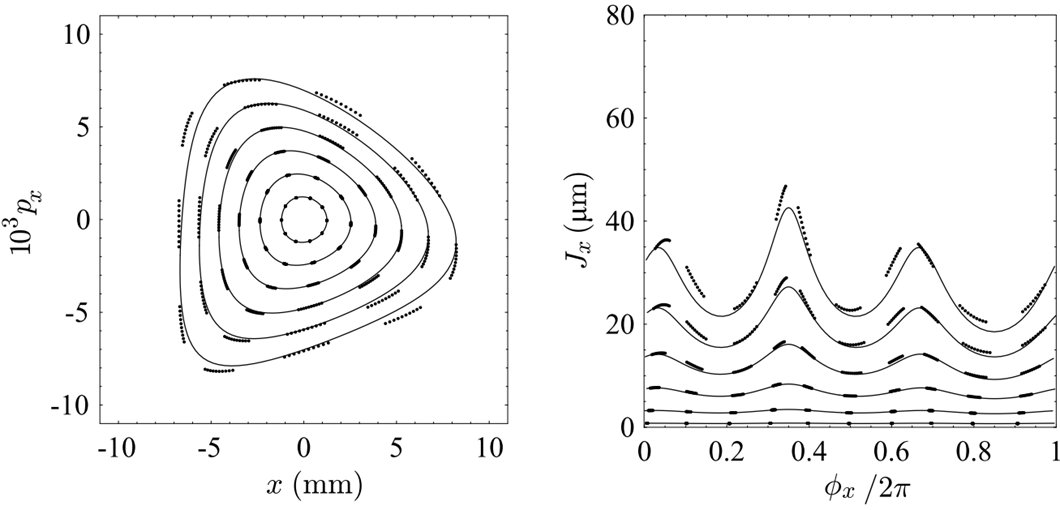
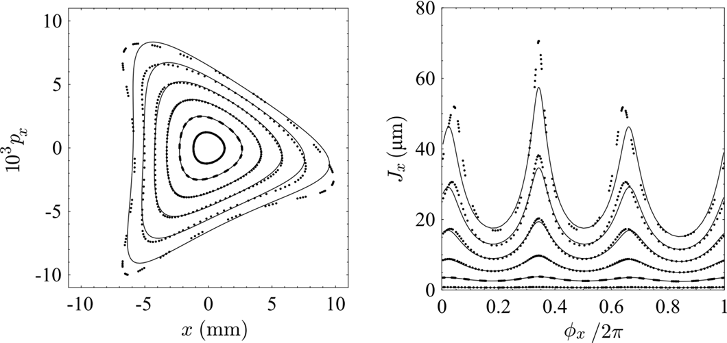
Power series maps are useful for particle tracking, but do not give much insight into the dynamics of a given nonlinear system. To develop a deeper understanding (for example, to determine the impact of individual resonances in a storage ring) more powerful techniques are needed. There are two approaches that are widely used in accelerator physics: perturbation theory [5, 6, 7], and normal form analysis [8, 9, 10]. In both these techniques, the goal is to construct a quantity that is invariant under application of the transfer map. Unfortunately, in both cases the mathematics is complicated and fairly cumbersome, and we do not discuss the details here. However, by way of illustration, consider the case of a simple storage ring containing a single sextupole in each periodic cell. Normal form analysis provides an expression for the betatron action $J_{x}$ of a particle in terms of the phase $\phi_{x}$ in this case [11]:

$$J_{x}\approx I_{0}-\frac{k_{2}L}{8}(2\beta_{x}I_{0})^{3/2}\frac{\left(\cos(3\mu_{x}/2+2\phi_{x})+\cos(\mu_{x}/2)\right)}{\sin(3\mu_{x}/2)}+O(I_{0}^{2}),$$

(94)

where $I_{0}$ is a constant (an invariant of the motion), $\phi_{x}$ is the angle variable, and $\mu_{x}$ is the phase advance per cell. Recall that the cartesian variables $x$, $p_{x}$ are related to the action–angle variables $J_{x}$, $\phi_{x}$ through Eqs. (12) and (13).

Note that the second term in the expression (94) for $J_{x}$ becomes very large when $\mu_{x}/2\pi$ is close to a third integer: this is the indication of a resonance. For linear motion, the action will be constant. The sextupoles in the lattice introduce some nonlinearity, which leads to a variation of the action as a particle moves around the ring (i.e. as the phase $\phi_{x}$ increases). The variation in the action becomes very large close to a third-order resonance. Although higher-order resonances may also be driven by the sextupoles, these are not shown in the expression in Eq. (94), which is based on normal form analysis carried out only up to a given order.

The phase space distortion (related to the variation in the betatron action as a function of angle) is illustrated in Fig. 20. Results from particle tracking (using a symplectic integrator) are shown as point on the plot; the variation in the action described by normal form analysis in Eq. (94) is shown as a solid line. Although there is not exact agreement, the normal form analysis does give a reasonable description of the dynamics, at least at low amplitude. Very large distortions (resulting from motion close to a resonance, or from a strongly-driven resonance, or at large amplitude) are difficult to describe analytically.

Close inspection of the plots in Fig. 20 reveals another effect, in addition to the obvious distortion of the phase space ellipses: the phase advance per turn (i.e. the tune) varies with increasing betatron amplitude. This effect is known simply as tune shift with amplitude. Normal form analysis and perturbation theory can both be used to obtain estimates for the size of the tune shift with amplitude, in terms of the coefficients of a series expansion for the tune in terms of the action:

$$\nu_{x}=\nu_{x0}+\left.\frac{\partial\nu_{x}}{\partial J_{x}}\right|_{J_{x}=0}J_{x}+\frac{1}{2}\left.\frac{\partial^{2}\nu_{x}}{\partial J_{x}^{2}}\right|_{J_{x}=0}J_{x}^{2}+\ldots$$

(95)

Note that in general, the tune in each plane (transverse horizontal and vertical) depends not just on the action in the corresponding plane, but also on the action in the opposite plane. One consequence of the fact that the motion (under appropriate conditions) is symplectic is that the horizontal tune shift with vertical amplitude is equal, or at least very close to, the vertical tune shift with horizontal amplitude.

Where the nonlinearity in a storage ring arises from a single sextupole in each periodic cell, the lowest order term in the expansion in Eq. (95) is second-order in the action. An octupole, however, does have a first-order tune shift with amplitude, given by:

$$\nu_{x}=\nu_{x0}+\frac{k_{3}L\beta_{x}^{2}}{16\pi}J_{x}+O(J_{x}^{2}),$$

(96)

where $k_{3}L$ is the integrated strength of the octupole, integrated over the length of the octupole:

$$k_{3}L=\frac{q}{P_{0}}\int_{0}^{L}\frac{\partial^{3}B_{y}}{\partial x^{3}}\,ds.$$

(97)

The tune shift with amplitude in a storage ring with a single octupole per cell becomes obvious if we construct a phase space portrait by tracking particles through a small number of cells: an example (for 30 cells) is shown in Fig. 21.

Tune shift with amplitude helps to explain the “islands” that we observed appearing in the phase space portraits for a storage ring with a single sextupole per periodic cell, see Fig. 10. The islands (closed loops around points away from the origin in phase space) are associated with resonances, and appear at amplitudes where the phase advance is $2\pi$ times a simple ratio of two integers, and where the transfer map contains an appropriate driving term for a resonance at the corresponding phase advance. The number of islands is determined by the denominator of the ratio of integers, and the width of the islands depends on the size of the tune shift with amplitude, and on the strength of the driving term.

For example, if we consider a one-turn map with a single octupole magnet and a linear map tuned for a phase advance close to a $4^{\textrm{th}}$ order resonance, we observe four stable islands in the phase space as shown in Fig. 22 (left). The tune shift with amplitude is illustrated in Fig. 22 (right), showing the tunes of the tracked particles as a function of their initial action ($2J_{x}$). Particles with small amplitude have tunes below the resonance. For large amplitudes, particles have tunes above the resonance and their tunes increase linearly with action. Particles trapped in the resonances islands have (on average) a tune locked to the resonance condition. As mentioned above, the width of the resonance islands depends on the tune shift with amplitude and on the resonance strength. This is also demonstrated in another case, where we consider a one-turn map consisting of a sextupole, an octupole and a linear map tuned to a phase advance of $\mu_{x}=0.328\times 2\pi$ (i.e. close to the $3^{\textrm{rd}}$ order resonance) as shown in Fig. 23. Here the phase space exhibits three stable islands. Note that the octupole induces a large tune shift with amplitude, which stabilises the particle motion at the resonance as it moves the particle tune out of the resonance for increasing amplitudes. For comparison, without the octupole and thus with a much smaller tune shift with amplitude, particles get lost at the same resonance as we have seen in Fig. 10.

References

- [1] S.Y. Lee, Accelerator Physics (World Scientific, 3rd edition, 2011).
- [2] A. Wolski, Beam Dynamics in High Energy Particle Accelerators (Imperial College Press, 2014).
- [3] H. Wiedemann, Particle Accelerator Physics (Springer, 4th edition, 2015).
- [4] D. Robin, C. Steier, J. Safranek, W. Decking, “Enhanced performance of the ALS through periodicity restoration of the lattice,” Proceedings of EPAC2000, Vienna, Austria (2000), pp. 136–140.
- [5] H. Goldstein, C.P. Poole Jr., J.L. Safko, Classical Mechanics (Pearson, 3rd edition, 2013).
- [6] R.D. Ruth, “Single particle dynamics and nonlinear resonances in circular accelerators”, in Nonlinear dynamics aspects of particle accelerators, Lecture Notes in Physics, Vol. 247 (Springer, 1986), pp. 37–63.
- [7] R.D. Ruth, “Single particle dynamics in circular accelerators”, Tech. Rep. SLAC–PUB–4103, (Stanford Linear Accelerator Center, 1986).
- [8] A.J. Dragt and J.M. Finn, “Normal form for mirror machine Hamiltonians”, Journal of Mathematical Physics 20 (1979), pp. 2649–2660.
- [9] F. Neri and A.J. Dragt, “Analysis of tracking data using normal forms”, Proceedings of the First European Particle Accelerator Conference, Rome, Italy (1988), pp. 675–677.
- [10] É. Forest, Beam Dynamics: A New Attitude and Framework (CRC Press, 1998).
- [11] Ibid. [2], pp. 373–384.
- [12] V.I. Arnold, Mathematical methods of classical mechanics (Springer, 2nd edition, 1989).
- [13] B.V. Chirikov, “A universal instability of many-dimensional oscillator systems”, Physics Reports 52, 5 (1979), pp. 263–379.
- [14] V.I. Arnold, “Instability of dynamical systems with several degrees of freedom”, Soviet Mathematics 5 (1964), pp. 581–588.
- [15] J. Laskar, “The chaotic motion of the solar system: a numerical estimate of the size of the chaotic zones”, Icarus 88 (1990), pp. 266–291.
- [16] J. Laskar, “Frequency map analysis of a Hamiltonian system”, Proceedings of “Nonlinear dynamics in particle accelerators: theory and experiments”, Arcidosso, Italy (1994), pp. 160–169.
- [17] J. Laskar, “Frequency map analysis and particle accelerators”, Proceedings of the 2003 Particle Accelerator Conference, Portland, OR, USA (2003), pp. 378–382.
- [18] L.N. Hand and J.D. Finch, Analytical mechanics, (Cambridge University Press, 1999).
- [19] S.G. Peggs and R.M. Talman, “Nonlinear problems in accelerator physics”, Ann. Rev. Nucl. Part. Sci. 36 (1986), pp. 287–325.
- [20] “A canonical integration technique”, IEEE Transactions on Nuclear Science, NS-30 (4) (1983), pp. 2669–2671.
- [21] “Geometric integration for particle accelerators”, J. Phys. A: Math. Gen. 39 (19) (2006), pp. 5321–5377.
- [22] “Fourth-order symplectic integration”, Physica D, 43 (1990).
- [23] “Construction of higher-order symplectic integrators”, Phys. Lett. A, 150 (1990).
- [24] E. Hairer, C. Lubich, G. Wanner, Geometric numerical integration, (Springer Series in Computational Mathematics, 2006).
- [25] H. Bartosik, G. Arduini, Y. Papaphilippou, “Optics considerations for lowering transition energy in the SPS”, Proceedings of the 2011 International Particle Accelerator Conference, San Sebastian, Spain (2011), pp. 619–621.
- [26] Y. Papaphilippou, “Detecting chaos in particle accelerators through the frequency map analysis method”, Chaos: An Interdisciplinary Journal of Nonlinear Science 24, 024412 (2014).
- [27] M.A. Palmer et al., “The conversion and operation of the Cornell Electron Storage Ring as a test accelerator (CesrTA) for damping rings research and development”, Proceedings of PAC09, Vancouver, BC, Canada (2009), pp. 4200–4204.
- [28] J. Laskar, “Introduction to frequency map analysis”, Proceedings of the NATO Advanced Studies Institute on “Hamiltonian systems with three or more degrees of freedom”, S’Agaro, Spain (1995), p. 134–150.