Deterministic improvements of quantum measurements with grouping of compatible operators, non-local transformations, and covariance estimates
Abstract
Obtaining the expectation value of an observable on a quantum computer is a crucial step in the variational quantum algorithms. For complicated observables such as molecular electronic Hamiltonians, a common strategy is to present the observable as a linear combination of measurable fragments. The main problem of this approach is a large number of measurements required for accurate estimation of the observable’s expectation value. We consider several partitioning schemes based on grouping of commuting multi-qubit Pauli products with the goal of minimizing the number of measurements. Three main directions are explored: 1) grouping commuting operators using the greedy approach, 2) involving non-local unitary transformations for measuring, and 3) taking advantage of compatibility of some Pauli products with several measurable groups. The last direction gives rise to a general framework that not only provides improvements over previous methods but also connects measurement grouping approaches with recent advances in techniques of shadow tomography. Following this direction, we develop two new measurement schemes that achieve a severalfold reduction in the number of measurements for a set of model molecules compared to previous state-of-the-art methods.
I Introduction
Variational Quantum Algorithms (VQA) constitute one of the most promising class of applications for quantum computers in the noisy intermediate scale quantum era. 1; 2 In VQAs, classically intractable optimization problems are represented as lowest eigenstates of -qubit operators
| (1) |
where ’s are coefficients and ’s are tensor products of Pauli operators or identities, . VQAs then solve these problems by minimizing where the quantum computer prepares the trial wavefunction and is given a task to measure , while a classical optimizer determines the optimal . However, it was found that estimating accurately for chemical systems requires large numbers of measurements that diminish VQA’s advantage over classical alternatives.3
Measuring is indeed not a straightforward task since only -Pauli operators can be measured on current digital quantum computers. A common approach to measuring the expectation value of the Hamiltonian is to present as a sum of measurable fragments . The condition for selecting ’s is that they can be easily rotated into polynomial functions of -Pauli operators
| (2) |
Then where the latter can be obtained by measuring -Pauli operators of for the rotated wavefunction .
Unfortunately, in general, the wavefunction is not an eigenstate of , and thus each fragment requires a set of measurements to obtain an estimator for . The efficiency of the Hamiltonian measurement scheme is determined by the total number of measurements, , needed to reach accuracy for . For a simple estimator of as the sum of estimators, the error scales as , where is the variance of each fragment, and ’s are the numbers of measurements allocated for each fragment, with the condition . The optimal distribution of measurements is , which gives the total estimator error as .
This consideration shows superiority of estimators operating with a set of measurable fragments that have the lowest sum over variance square roots. For practical use of this consideration, there are two difficulties in explicit optimization of the estimator error: 1) there is an overwhelming number of choices for measurable operator fragments and 2) variance estimates require knowledge of the wavefunction. The second problem can be addressed by introducing a classically efficient proxy for the quantum wavefunction (e.g. from Hartree-Fock or configuration interaction singles and doubles (CISD) methods in quantum chemistry problems) or by utilizing the measurement results from VQAs to gain empirical estimates. Yet, the search space in the first problem is so vast that it has only been addressed heuristically in previous studies. The Hamiltonian partitioning has been done in qubit space4; 5; 6; 7; 8; 9; 10; 11 and in the original fermionic space with subsequent transfer of all operators into the qubit space.12; 13 An initial heuristic idea was to reduce the number of measurable fragments without accounting for variances. It was shown for several partitioning that the number of fragments is not a good proxy for the total number of measurements, and the fragments’ variances cannot be ignored.14; 13 The key element determining a particular set of measurable fragments is a class of unitary transformations ’s in Eq. (2). Compared to single-qubit transformations, multi-qubit transformations are more flexible and therefore have a greater potential to minimize the total number of measurements by selecting fragments with lower variances. Yet, they also have a downside of an extra circuit overhead needed to perform the rotation before the measurement. Once the set of unitary transformations has been selected, empirically, it was found more beneficial for the estimator variance to use greedy algorithms for the Hamiltonian partitioning. In these algorithms one finds fragments sequentially by minimizing the norm of the difference between partial sum of ’s and .14; 13 This can be rationalized considering that greedy algorithms produce first fragments with larger variances and later fragments with smaller variances. Such a distribution of variances makes sum of square roots somewhat smaller compare to the case where variances are distributed relatively equally over all fragments.
Fragmentation techniques in the qubit space are based on grouping mutually commuting Pauli products in each fragment [Eq. (2)]. Two types of commutativity between Pauli products are used: qubit-wise and full commutativity. The full commutativity (FC) is the regular commutativity of two operators,7 whereas the qubit-wise commutativity (QWC) for two Pauli products is a condition when corresponding single-qubit operators commute.5 Using either commutativity to find ’s, one can efficiently identify unitary operators ’s from the Clifford group that bring the fragments to the form of Eq. (2) for measurement. Only one-qubit Clifford gates are sufficient for ’s of the qubit-wise commuting fragments,5 while ’s for fully commuting fragments require also two-qubit Clifford gates.7
Initial QWC- and FC-based schemes had ’s consisting of disjoint (non-overlapping) sets of Pauli products. Generally, each Pauli product can belong to multiple ’s as long as it commutes with all terms in these fragments. This follows from non-transitivity of both FC and QWC as binary relations: if commutes with , and commutes with , this does not lead to commutativity of and . For the measurement problem, and form separate measurable groups while can be measured within both of these groups. Here, constitutes an overlapping element for the and groups (see Fig. 1 where , , and are , , and respectively). Recent developments based on shadow tomography 15; 16; 17; 18 and grouping19; 20 techniques exploiting overlapping fragments found considerable reduction in the number of needed measurements over non-overlapping grouping schemes. However, all non-overlapping schemes used in those comparisons did not use the greedy approach. Since within qubit-based partitioning schemes there are multiple estimator improvement techniques, it is interesting to assess them all systematically.
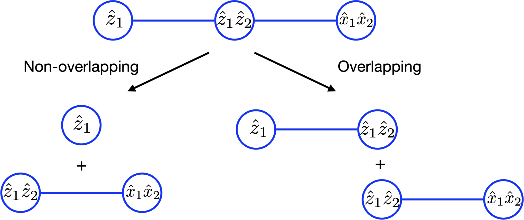
In this work, we assess improvements in the total number of measurements from introducing a series of ideas: 1) grouping commuting operators using the greedy approach, 2) involving non-local (entangling) unitaries for measuring groups of fully commuting Pauli products, and 3) taking advantage of compatibility of some Pauli products with several measurable groups (i.e. overlapping grouping). It is shown that these ideas, used separately or combined, can give rise to schemes superior to prior art within grouping and shadow tomography techniques. One of the most striking findings is that using only greedy non-overlapping grouping within the QWC approach can already surpass the performance of recent shadow tomography techniques that employed overlapping local frames. We do not consider fermionic-algebra-based techniques here because they do not allow overlapping grouping while all other improvements were already discussed for them.13 Other measurement techniques that do not involve grouping of Hamiltonian terms are also outside of the scope of the current work. 21; 22; 23; 24; 25
II Theory
II.1 Estimator for non-overlapping Pauli groups
All measurable fragments ’s are linear combinations of mutually commuting or qubit-wise commuting Pauli products
| (3) |
where ’s are disjoint sets of Pauli products measured as parts of corresponding ’s, and ’s are coefficients of ’s in the Hamiltonian. The commutativity between Pauli products within implies a common eigen-basis , where one can measure all the members of . Initial proposals to find these fragments aim to minimize the total number of fragments using graph coloring algorithms, such as the largest first (LF) algorithm. 5; 7 But later the sorted insertion (SI) algorithm employing the greedy approach was found to produce lower variances for the energy estimator. 14
Let denote the estimator for ; it is a sum of estimators for its parts
| (4) |
Each comes from repeated measurements of ,
| (5) |
where is the -th measurement result of . The variance of is
| (6) |
where ’s are variances of estimators characterizing differences between ’s and the true expectation values ’s. Note that covariances between different fragments are zero because measurements of different fragments are done independently. ’s can be evaluated using quantum operator variances ’s, , which leads to the Hamiltonian estimator variance as
| (7) |
Using the constraint one can minimize with respect to ’s26; 14
| (8) | |||||
| (9) |
In practice, quantum variances are not known a priori. They can be evaluated using covariances between Pauli products,
| (10) | |||||
| (11) | |||||
where . The covariances for different Pauli products are generally non-zero because all of these Pauli products are measured together within the same fragment. The covariances can be approximated for molecular Hamiltonians using approximate wavefunctions obtained on a classical computer. Configuration interaction singles and doubles (CISD) is one example for obtaining approximation for that will be used in the current work. Alternatively, the measurements results obtained from measurement basis can help estimate the covariances between Pauli products of during VQA’s cycles.
II.2 Optimization by Coefficient Splitting
Many Pauli products in the Hamiltonian can be measured in multiple fragments because of their compatibility with other members of those fragments. The coefficient splitting approach, briefly mentioned in Ref. 14, takes advantage of this opportunity by splitting coefficients of Pauli products that are compatible with multiple fragments
| (12) | |||||
| (13) |
where is a set of group indices corresponding to fragments whose members are compatible with (see Fig. 1 for an example). Note that the equations for the estimator variance and the optimal measurement distribution remain the same [Eqs. (8) and (9)]. However, freedom in the coefficient splitting approach [Eq. (13)] can be used to minimize the Hamiltonian estimator variance [(9)].
A straightforward approach to minimization of with respect to ’s is to use analytical gradients . The gradients are non-linear functions of and computing them becomes computationally expensive as the number of ’s grows with the size of the system. As a computationally more efficient alternative, we propose an iterative heuristic that quickly converges to a zero gradient solution.
Iterative coefficient splitting (ICS): Given a particular choice of ’s and its optimal ’s, the procedure consists of iteratively applying two steps: (1) optimization of ’s with fixed ’s and (2) optimization of ’s with fixed ’s. The second step is straightforward using Eq. (8). For the first step, notice that when ’s is fixed, the derivatives of with respect to ’s are linear in ’s:
To account for the constraints in Eq. (13), for each splitting of , we fix one of the as . The gradients become
| (14) | |||||
This allows us to find an optimal ’s by solving the linear system of equations obtained by equating the gradients to zero.
If the number of ’s overcomes computationally affordable limits, one can always limit the minimization to a selected subset of ’s. The criteria for the suitable subset could be the variances, which correlate with magnitudes of their covariances and therefore the importance of their coefficients for .
II.3 Optimization by Measurement Allocation
Another approach to reducing the Hamiltonian estimator variance is to measure each Pauli product as a member of as many compatible measurable fragments as possible. This idea was used in classical shadow tomography methods based on local transformations for measurement of Pauli products.15; 16; 19 First, for a particular Pauli product , one finds a set of measurement bases ’s where can be measured (see Fig. 1 for an example, by a measurement group this method considers a set of compatible Pauli products). Then, all measurement results for obtained in ’s are used to estimate :
| (15) |
where is the -th measurement result of measured in basis , and is the total number of times is measured. ’s are used in the Hamiltonian estimator as . The variance of is
| (16) | |||||
| (17) |
To proceed further, it is important to distinguish covariances between Pauli products measured within the same fragment and in different fragments. The former correspond to and in Eq. (17) and generally are non-zero, while the latter ( or ) are zero
| (18) | |||||
Note that the key element in deriving this Hamiltonian estimator variance is the consideration that if a Pauli product is measured as a part of a certain group, all members of this group contribute to the average and to the variance. Thus, the variance of each group gives rise to covariances between its members. Since the covariances in different groups are different in magnitude, placing a particular Pauli product in all compatible groups can be sub-optimal for the total variance of the Hamiltonian estimator.
Dependencies of and on ’s in [Eq. (18)] make finding the optimal measurement allocation in the analytic form infeasible. To minimize with respect to ’s in Eq. (18) one can numerically optimize ’s as positive variables with restriction . We will refer to this strategy as the measurement allocation approach. It turns out that such minimization is a version of the coefficient splitting approach with . Indeed, substituting ’s for ’s in and using Eq. (7), we obtain as
| (19) | |||||
which agrees with Eq. (18). Therefore, the measurement allocation approach can be seen as a particular choice of coefficient splitting for reducing . The main advantage of the measurement allocation approach is a much lower number of optimization variables () compared to that of the coefficient splitting scheme ().
One can formulate approximation for gradients of with respect to continuous proxy of ’s (see Appendix A), which leads to a gradient descent scheme that we will refer to as gradient-based measurement allocation (GMA). Yet, a computationally more efficient, non-gradient iterative scheme was found and detailed below.
Iterative measurement allocation (IMA): Given an initial guess for ’s and resulting ’s, the corresponding coefficient splitting partitioning of the Hamiltonian is
| (20) |
where
| (21) |
Recall that the optimal measurement allocation for any coefficient splitting is given by Eq. (8). Thus, we use this optimal allocation to update ’s as
| (22) |
which leads to the update in measurable groups
| (23) |
Since there is no guarantee that each iteration will necessarily lower in Eq. (18), we repeat these steps multiple times and choose ’s that result in the lowest estimator variance. Empirically, the procedure finds the best measurement allocation in first few cycles.
III Results and Discussions
We assess the performance of the proposed approaches (IMA, GMA, and ICS) in comparison to prior works (LF, SI, and classical-shadow-based algorithms) in estimating energy expectation values for ground eigen-states of several molecular electronic Hamiltonians. 27 To compare different schemes, we normalize the total measurement budget and require ’s to be positive real numbers. The estimator variance with ’s, , can be scaled by to approximate the estimator variance for measurements for each group. The overlapping groups (’s) of the proposed methods are obtained from an extension of the SI technique (see Appendix B). The initial measurement allocations or coefficient splittings are derived from measurement allocations of the SI technique using exact or CISD wavefunctions.
To illustrate the relative performance of our methods, Table 1 presents the Hamiltonian estimator variances based on covariances calculated with the exact wavefunction. Lower variances in SI compared to those in LF are consistent with earlier findings 14. All proposed methods result in lower variances than those in SI. As the most flexible approach, the coefficient splitting method ICS achieves the lowest variances. GMA has a slight edge over IMA in estimator variances, but due to the computational cost of GMA, we will only consider IMA from here on.
Table 2 shows the number of optimization variables in the measurement allocation and coefficient splitting techniques. For the measurement allocation approaches (IMA and GMA) the number of variables is equal to the number of measurable groups. For the qubit-wise (full) commutativity, the number of such groups scales as () since on average each group contains three () Pauli products. For relatively small molecules in our set (i.e. only few atoms), scales as . In the coefficient splitting approach, the number of variables is a product of and an average number of measurable groups that are compatible with an average Pauli product. For our model systems, it was found empirically that the latter number grows as for the qubit-wise commutativity, whereas for the full commutativity the number is within a range of and thus can be considered relatively constant. These considerations clarify why the measurement allocation techniques can be employed for both commutativities, but the coefficient splitting without extra constraints can be afforded only for the FC grouping.
| Systems | LF | SI | IMA | GMA | ICS |
|---|---|---|---|---|---|
| Qubit-wise commutativity | |||||
| H2 | 0.136 | 0.136 | 0.136 | 0.136 | 0.136 |
| LiH | 5.84 | 2.09 | 1.73 | 1.52 | 0.976 |
| BeH2 | 14.3 | 6.34 | 5.60 | 5.26 | 4.29 |
| H2O | 116 | 48.6 | 27.9 | 18.8 | 13.5 |
| NH3 | 352 | 97.0 | 83.3 | 62.1 | 44.8 |
| Full commutativity | |||||
| H2 | 0.136 | 0.136 | 0.136 | 0.136 | 0.136 |
| LiH | 1.43 | 0.882 | 0.647 | 0.517 | 0.232 |
| BeH2 | 5.18 | 1.11 | 1.02 | 0.974 | 0.459 |
| H2O | 43.4 | 7.59 | 5.88 | 4.27 | 1.50 |
| NH3 | 78.7 | 18.8 | 13.6 | 9.35 | 3.32 |
| Systems | QWC | FC | ||||
|---|---|---|---|---|---|---|
| MA | CS | MA | CS | |||
| H2 | 4 | 15 | 3 | 4 | 2 | 6 |
| LiH | 12 | 631 | 155 | 3722 | 42 | 1466 |
| BeH2 | 14 | 666 | 183 | 5946 | 36 | 1203 |
| H2O | 14 | 1086 | 334 | 11192 | 50 | 1823 |
| NH3 | 16 | 3609 | 1359 | 61137 | 122 | 6138 |
To compare the proposed methods to the classcial shadow tomography techniques (Derand16 and OGM19), we consider QWC grouping methods that do not require non-local (entangling) transformations (Table 3). Unlike the original OGM treatment, we avoid deleting measurement bases to compare all methods on an equal footing. Comparison between the non-overlapping techniques (LF and SI) and classical shadow techniques reveals that only employing the greedy approach to QWC grouping in SI is already enough to surpass the classical shadow tomography techniques. In accord with results of Table 1, both IMA and ICS outperform SI even when approximate covariances are used.
Lastly, we present improvements on the variances that can be achieved by adopting non-local unitary transformations and FC grouping (Table 4). For all considered systems, IMA and ICS are superior to SI. This shows that approximate covariances based on the CISD wavefunction can perform similarly to the exact ones.
| Systems | LF | OGM | Derand | SI | IMA | ICS |
|---|---|---|---|---|---|---|
| H2 | 0.136 | 0.173 | 0.144 | 0.136 | 0.136 | 0.136 |
| LiH | 5.84 | 3.50 | 3.74 | 2.09 | 1.73 | 0.978 |
| BeH2 | 14.3 | 18.3 | 12.5 | 6.34 | 5.60 | 4.40 |
| H2O | 166 | 148 | 114 | 48.6 | 27.9 | 13.8 |
| NH3 | 500 | 305 | 251 | 97.0 | 83.4 | 45.5 |
| Systems | LF | SI | IMA | ICS |
|---|---|---|---|---|
| H2 | 0.136 | 0.136 | 0.136 | 0.136 |
| LiH | 1.43 | 0.882 | 0.647 | 0.232 |
| BeH2 | 5.19 | 1.11 | 1.02 | 0.495 |
| H2O | 43.4 | 7.59 | 5.89 | 1.68 |
| NH3 | 78.8 | 18.8 | 13.7 | 3.42 |
IV Conclusions
We assessed multiple ideas for reduction of the number of measurements required to accurately obtain the expectation value of any operator that can be written as a sum of Pauli products. Since these ideas can be used separately or combined, our main goal was to understand the impact on the number of measurements and incurred computational cost of each idea. Exploring the idea of Pauli products’ compatibility led to the realization that the coefficient splitting framework is the most general implementation of this idea for the grouping methods.
We found that although classical shadow techniques have shown performance superior to that of the non-overlapping measurement scheme based on graph-coloring algorithms, by employing a greedy heuristic the non-overlapping scheme can already outperform the classical shadow techniques. Due to the dependence of the total number of measurements on the sum of square roots of variances for measurable fragments, the greedy approach to grouping performs the best by creating distributions of fragments that are highly non-uniform in variance. The SI technique based on greedy grouping and using only qubit-wise commutativity surpasses shadow tomography based techniques (Derand and OGM) by a factor of 2-3 for larger systems. Thus, for future developments, the shadow tomography approaches need to be compared with greedy grouping based algorithms rather than with grouping approaches that try to minimize the overall number of measurable groups (e.g. LF).
Unlike previous classical shadow techniques that focus on qubit-wise commuting groups, we also considered measuring techniques involving non-local (entangling) transformations that allow one to measure groups of fully commuting Pauli products. An efficient implementation of these non-local transformations using Clifford gates was proposed by Gottesman28 and would introduce only CNOT gates. The schemes based on fully commuting groups outperform their qubit-wise commuting counterparts up to a factor of seven in variances of the expectation value estimators.
Taking advantage of compatibility of some Pauli products with members of multiple measurable groups (i.e. overlapping groups idea) can be generally presented as augmenting the measurable groups with all Pauli products compatible with initial members of these groups. Then the coefficients of Pauli products entering multiple groups are optimized to lower the estimator variance, with the constraint that the sum over coefficients in different groups for each Pauli product is equal to the coefficient of the Pauli product in the Hamiltonian. This coefficient splitting approach incorporates as a special case a heuristic technique of optimizing measurement allocation for overlapping measurable groups.
Even though the coefficient splitting variance minimization provides the lowest variances among all studied approaches, it requires optimizing a large number of variables: () for full (qubit-wise) commutativity. Due to certain restrictions, the measurement allocation approach is much more economical in the number of optimization variables: () for full (qubit-wise) commutativity. Another contributor of the computational cost of these techniques is calculation of the variance gradients. To reduce the computational cost of this part we proposed iterative schemes, the ICS method converges to true extrema, while the IMA scheme deviates from extrema. IMA and ICS provide up to forty and eighty percent reduction in the number of measurements required compared to corresponding best non-overlapping techniques.
Both IMA and ICS use approximate covariances between Pauli products to lower the estimator variance. Use of CISD wavefunction for calculating these covariances shown improvements comparable to those obtained using the exact covariances. Additionally, in IMA and ICS, one can improve covariances obtained from approximate wavefunctions using accumulated measurement results.
Data Availability
The data that support the findings of this study are available from the corresponding author upon request.
Code Availability
Acknowledgements
T.Y. is grateful to Hsin-Yuan Huang and Bujiao Wu for providing details of their respective algorithms in Refs. 16 and 19. The authors thank Seonghoon Choi for useful discussion. A.F.I. acknowledges financial support from the Google Quantum Research Program, Early Researcher Award, and Zapata Computing Inc. This research was enabled in part by support provided by Compute Ontario and Compute Canada.
Author Contributions
T.-C.Y. and A.F.I conceptualized the project and wrote most of the paper. A.G. developed IMA and collected all the data, except for calculations of LF (in Table. 1), SI (in Table. 1), GMA, and OGM that T.-C.Y. performed. T.-C.Y., A.G., and A.F.I participated in discussions that developed the theory as well as the GMA and ICS methods. T.-C.Y. and A.G. share co-first authorship.
Competing Interests
The authors declare that there are no competing interests.
Appendix A Gradients of Measurement Allocation Optimization
The variance of the estimator for as a function of ’s and ’s is
| (24) |
| (25) | |||||
Note that ’s are dependent on ’s. We minimize using ’s as variables under the constraints and . The variance derivatives with respect to ’s are
| (26) | |||||
To avoid constrained optimization with ’s, we use auxiliary variables ’s that express ’s as
| (27) |
to introduce the and conditions. This is known as the softmax function often used in machine learning techniques. Derivatives only require additional terms
| (28) |
for completing a chain-rule expression with Eq. (26).
Appendix B Extensions of Sorted Insertion
Sorted Insertion (SI)14 is one of the most efficient measurement schemes that utilizes non-overlapping Pauli groups. Here, we briefly review the original implementation and introduce modifications to find overlapping groups for the coefficient splitting and measurement allocation approaches.
SI partitions all the Pauli products in into a set of non-overlapping groups such that
| (29) | |||||
| (30) |
SI initiates , and finds the partitioning through the following steps:
- 1.
Sort Pauli products in in the descending order of the magnitudes of their coefficients.
- 2.
Examine each product . If commutes with all products in ,
(31) (32) - 3.
Add to . Set and repeat from step 2 until is empty.
In order to obtain overlapping groups, we maintain set to track Pauli products that are already part of some fragments, and examine whether they are compatible with the group built in step 2. Note that the order in which the Pauli products are added to the groups matters, since the additional Pauli products that are compatible with the SI groups may not be compatible between themselves. We initiate and add an extra procedure between step 2 and 3:
- •
For in the order they were added to , add to if is compatible with all members of . Then, , in the order added to , set
References
- Preskill (2018) J. Preskill, Quantum Computing in the NISQ era and beyond, Quantum 2, 79 (2018).
- Peruzzo et al. (2014) A. Peruzzo, J. McClean, P. Shadbolt, M.-H. Yung, X.-Q. Zhou, P. J. Love, A. Aspuru-Guzik, and J. L. O’Brien, A variational eigenvalue solver on a photonic quantum processor, Nat. Commun. 5, 4213 (2014).
- Gonthier et al. (2020) J. F. Gonthier, M. D. Radin, C. Buda, E. J. Doskocil, C. M. Abuan, and J. Romero, Identifying challenges towards practical quantum advantage through resource estimation: the measurement roadblock in the variational quantum eigensolver, arXiv.org , arXiv:2012.04001 (2020), 2012.04001 .
- Izmaylov et al. (2019) A. F. Izmaylov, T.-C. Yen, and I. G. Ryabinkin, Revising the measurement process in the variational quantum eigensolver: is it possible to reduce the number of separately measured operators?, Chem. Sci. 10, 3746 (2019).
- Verteletskyi et al. (2020) V. Verteletskyi, T.-C. Yen, and A. F. Izmaylov, Measurement optimization in the variational quantum eigensolver using a minimum clique cover, J. Chem. Phys. 152, 124114 (2020).
- Jena et al. (2019) A. Jena, S. Genin, and M. Mosca, Pauli Partitioning with Respect to Gate Sets, arXiv.org , arXiv:1907.07859 (2019), 1907.07859 .
- Yen et al. (2020) T.-C. Yen, V. Verteletskyi, and A. F. Izmaylov, Measuring all compatible operators in one series of a single-qubit measurements using unitary transformations, J. Chem. Theory Comput. 16, 2400 (2020).
- Gokhale et al. (2020) P. Gokhale, O. Angiuli, Y. Ding, K. Gui, T. Tomesh, M. Suchara, M. Martonosi, and F. T. Chong, Measurement Cost for Variational Quantum Eigensolver on Molecular Hamiltonians, IEEE Transactions on Quantum Engineering 1, 1 (2020).
- Izmaylov et al. (2020) A. F. Izmaylov, T.-C. Yen, R. A. Lang, and V. Verteletskyi, Unitary partitioning approach to the measurement problem in the variational quantum eigensolver method, J. Chem. Theory Comput. 16, 190 (2020).
- Zhao et al. (2020) A. Zhao, A. Tranter, W. M. Kirby, S. F. Ung, A. Miyake, and P. J. Love, Measurement reduction in variational quantum algorithms, Phys. Rev. A 101, 062322 (2020).
- Hamamura and Imamichi (2020) I. Hamamura and T. Imamichi, Efficient evaluation of quantum observables using entangled measurements, npj Quantum Information 6, 10.1038/s41534-020-0284-2 (2020).
- Huggins et al. (2021) W. J. Huggins, J. McClean, N. Rubin, Z. Jiang, N. Wiebe, K. B. Whaley, and R. Babbush, Efficient and Noise Resilient Measurements for Quantum Chemistry on Near-Term Quantum Computers, npj Quantum Inf 7, 23 (2021).
- Yen and Izmaylov (2021) T.-C. Yen and A. F. Izmaylov, Cartan subalgebra approach to efficient measurements of quantum observables, PRX Quantum 2, 040320 (2021).
- Crawford et al. (2021) O. Crawford, B. v. Straaten, D. Wang, T. Parks, E. Campbell, and S. Brierley, Efficient quantum measurement of Pauli operators in the presence of finite sampling error, Quantum 5, 385 (2021).
- Hadfield et al. (2020) C. Hadfield, S. Bravyi, R. Raymond, and A. Mezzacapo, Measurements of quantum hamiltonians with locally-biased classical shadows, arXiv.org , arXiv:2006.15788 (2020), 2006.15788 .
- Huang et al. (2021) H.-Y. Huang, R. Kueng, and J. Preskill, Efficient estimation of pauli observables by derandomization, Phys. Rev. Lett. 127 (2021).
- Hillmich et al. (2021) S. Hillmich, C. Hadfield, R. Raymond, A. Mezzacapo, and R. Wille, Decision diagrams for quantum measurements with shallow circuits (2021), arXiv:2105.06932 [quant-ph] .
- Hadfield (2021) C. Hadfield, Adaptive pauli shadows for energy estimation (2021), arXiv:2105.12207 [quant-ph] .
- Wu et al. (2021) B. Wu, J. Sun, Q. Huang, and X. Yuan, Overlapped grouping measurement: A unified framework for measuring quantum states, arXiv.org , arXiv:2105.13091 (2021), 2105.13091 .
- Shlosberg et al. (2021) A. Shlosberg, A. J. Jena, P. Mukhopadhyay, J. F. Haase, F. Leditzky, and L. Dellantonio, Adaptive estimation of quantum observables (2021), arXiv:2110.15339 [quant-ph] .
- Radin and Johnson (2021) M. D. Radin and P. Johnson, Classically-Boosted Variational Quantum Eigensolver (2021), arXiv:2106.04755 [quant-ph] .
- Bespalova and Kyriienko (2021) T. A. Bespalova and O. Kyriienko, Hamiltonian Operator Approximation for Energy Measurement and Ground-State Preparation, PRX Quantum 2, 030318 (2021).
- Wang et al. (2021) G. Wang, D. E. Koh, P. D. Johnson, and Y. Cao, Minimizing Estimation Runtime on Noisy Quantum Computers, PRX Quantum 2, 010346 (2021).
- Torlai et al. (2020) G. Torlai, G. Mazzola, G. Carleo, and A. Mezzacapo, Precise measurement of quantum observables with neural-network estimators, Phys. Rev. Research 2, 022060 (2020).
- García-Pérez et al. (2021) G. García-Pérez, M. A. Rossi, B. Sokolov, F. Tacchino, P. K. Barkoutsos, G. Mazzola, I. Tavernelli, and S. Maniscalco, Learning to measure: Adaptive informationally complete generalized measurements for quantum algorithms, PRX Quantum 2, 040342 (2021).
- Rubin et al. (2018) N. C. Rubin, R. Babbush, and J. McClean, Application of fermionic marginal constraints to hybrid quantum algorithms, New Journal of Physics 20, 053020 (2018).
- (27) The qubit Hamiltonians were generated using the STO-3G basis and the BK transformation. The nuclear geometries for the Hamiltonians are R (), R (), R with collinear atomic arrangement (), R with (), and R with ().
- Aaronson and Gottesman (2004) S. Aaronson and D. Gottesman, Improved simulation of stabilizer circuits, Phys. Rev. A 70, 052328 (2004).
- McClean et al. (2019) J. R. McClean, K. J. Sung, I. D. Kivlichan, Y. Cao, C. Dai, E. S. Fried, C. Gidney, B. Gimby, P. Gokhale, T. Häner, T. Hardikar, V. Havlíček, O. Higgott, C. Huang, J. Izaac, Z. Jiang, X. Liu, S. McArdle, M. Neeley, T. O’Brien, B. O’Gorman, I. Ozfidan, M. D. Radin, J. Romero, N. Rubin, N. P. D. Sawaya, K. Setia, S. Sim, D. S. Steiger, M. Steudtner, Q. Sun, W. Sun, D. Wang, F. Zhang, and R. Babbush, Openfermion: The electronic structure package for quantum computers (2019), arXiv:1710.07629 [quant-ph] .
- Sun et al. (2018) Q. Sun, T. C. Berkelbach, N. S. Blunt, G. H. Booth, S. Guo, Z. Li, J. Liu, J. D. McClain, E. R. Sayfutyarova, S. Sharma, S. Wouters, and G. K.-L. Chan, Pyscf: the python-based simulations of chemistry framework, WIREs Computational Molecular Science 8, e1340 (2018).