PDRs4all: NIRSpec simulation of integral field unit spectroscopy of the Orion Bar photodissociation region

Amélie Canin OrcID: 0000-0002-7830-6363 Affiliation: Institut de Recherche en Astrophysique et Planétologie (IRAP), University of Toulouse, France. olivier.berne@irap.omp.eu Olivier Berné OrcID: 0000-0002-1686-8395 Affiliation: Institut de Recherche en Astrophysique et Planétologie (IRAP), University of Toulouse, France. olivier.berne@irap.omp.eu The PDRs4All ERS team

Abstract

The James Webb Space Telescope (JWST) was launched on December 25 2021. This document presents a simulation of the Near Infrared Spectrograph (NIRSpec) observations of the Orion Bar which will be performed as part of the Early Release Sciences (ERS) program “PDRs4all”. The methodology to produce this data relies on the use of a direct forward model of the instrument applied to a synthetic scene of the Orion Bar, coupled to format matching in order to deliver data in JWST-pipeline data format. The resulting 3D cube for one order is provided publicly, and is compatible with tools developed by the STScI (e.g. Cubeviz) and with the science enabling products developed by the PDRs4all team. This cube can be used as a template observation for proposers who would like to apply for NIRSpec observations of extended sources with JWST.

I Introduction

The James Webb Space Telescope (Gardner et al. 2006, JWST) is a space telescope developed jointly by NASA, European Space Agency (ESA) and Canadian Space Agency (CSA). This telescope, launched on December 25, 2021, has four main scientific focuses: ‘‘The End of the Dark Ages: First Light and Reionization”; ‘‘The Assembly of Galaxies”; ‘‘The Birth of Stars and Protoplanetary Systems”; and ‘‘Planetary Systems and the Origins of Life”. Thirteen Early Release Science (ERS) programs have been selected to demonstrate the scientific capabilities of JWST, to provide public data to the community, to educate and inform the community regarding JWST’s capabilities. This paper is part of this effort in the context of the ERS program “PDRs4all: Radiative feedback from massive stars”¹¹ 1 http://pdrs4all.org (ID1288) which focuses on observations of the Orion Nebula (Berné et al. 2022). This 40-hour program will make use of three instruments aboard JWST, and will dedicate about 12.71 hours to spectroscopy of the Orion Bar with the Near Infrared Spectrograph (NIRSpec, Bagnasco et al. 2007). The NIRSpec instrument (Bagnasco et al. 2007) has 9 filters between 0.6 $\mu$ m and 5.27 $\mu$ m out of which we will use 3 in the PDRs4all ERS project.

In this paper, we present a method to simulate NIRSpec hyperspectral images of the Orion Bar as planned in this ERS project, in the JWST pipeline format. The goal of these simulations is to prepare the tools that post-process the pipeline output and to test the ecosystem of analysis tools developed for JWST data²² 2 https://jwst-docs.stsci.edu/jwst-post-pipeline-data-analysis. The paper is organised as follows: Section II gives an overview of the NIRSpec instrument. In Section III, we present how we simulate the NIRSpec image following Guilloteau et al. 2020, and make it compatible with the NIRSpec output pipeline format.

II NIRSpec Spectroscopy of the Orion Bar

The Near Infrared Spectrograph (NIRSpec, Bagnasco et al. 2007) is one of the four JWST instruments. There are four observing modes of NIRSpec and we are specifically interested in the imaging spectroscopy with the Integral Field Unit (IFU)³³ 3 For more information: https://jwst-docs.stsci.edu/jwst-near-infrared-spectrograph.

The IFU mode has 9 disperser-filter combinations that span a total wavelength range of $0.6\mu m$ to $5.3\mu m$ , and provide three levels of resolving power⁴⁴ 4 More information on IFU mode: https://jwst-docs.stsci.edu/jwst-near-infrared-spectrograph/nirspec-observing-modes/nirspec-ifu-spectroscopy. As part of the PDRs4all ERS project, 6 NIRSpec observations are planned with 3 disperser-filter combinations covering wavelengths between $0.97\mu m$ and $5.27\mu m$ with a nominal resolving power of 2,700. Each exposure will have one integration and each integration will consist of 5 groups with 4 dithers giving a total integration time of $257.68s$ . The footprints of these NIRSpec observations as specified in the Astronomer’s Proposal Tool (APT⁵⁵ 5 https://jwst-docs.stsci.edu/jwst-astronomers-proposal-tool-overview) positioned over the Orion Bar are shown in Fig. 1.

Refer to caption — Figure 1: NIRSpec field of view for the PDRs4all project as specified in the ERS 1288 APT file, with HST-WFC3 (Kimble et al. 2008) with the F656N filter (6.56 $\mu$ m) image of the Orion star forming region in background. Blue regions: NIRSpec footprints corresponding to planned observations. Red cross: position of the target at the coordinates R.A. = 5:35:20.4749, dec. = -5:25:10.45.

III Simulation

III.1 Motivation and strategy

Creating NIRSpec simulations is useful to test JWST analysis tools developed by the PDRs4all team (Berné et al. 2022) or by other teams including those of the STScI (e.g. Cubeviz, Jones et al. 2019). These simulations are also useful to obtain an idea of the quality (in terms of SNR) and richness of the data for a given integration time, ahead of observations. However, performing such simulations is challenging. There exists an instrument simulator (Piquéras et al. 2010), however simulating a full 3D NIRSpec cube (i.e. two spatial dimensions and one spectral dimension) with realistic spatial and spectral textures using this tool is very computationally intensive. As part of a project to develop algorithms to perform data-fusion between NIRSpec and NIRCam, these authors have created a forward mathematical model of the NIRSpec instrument. They applied this forward model to a 3 dimensional input synthetic scene of the Orion Bar to create realistic NIRSpec simulations over the $1\mu m$ to $2.35\mu m$ wavelength range. As part of the PDRs4all project, a larger wavelength range is expected to be observed ( $0.97\mu m$ to $5.2\mu m$ ) with NIRSpec. In addition, Guilloteau et al. 2020 did not implement any tools to write out the cubes in the JWST pipeline format. In this paper, we present how we have extended the method of Guilloteau et al. 2020. To obtain a NIRSpec IFU simulated cube, we apply the direct model of Guilloteau et al. 2020 on the Orion Bar synthetic scene including the $0.97\mu m$ to $5.2\mu m$ range, and from this simulation we extract a cube with precisely the properties of the JWST-NIRSpec pipeline. We thus produce a realistic simulated IFU NIRSpec cube in the stage 3 format of the JWST-NIRSpec pipeline.

III.2 Choice of region to be simulated

Fig. 1 presents an overview of the footprints of the NIRSpec IFU observations planned in September 2022 on the Orion Bar as part of PDRs4all. They span a cut across the Orion Bar, performed with a mosaic strategy (see Berné et al. 2022). Fig. 2 is a zoomed-in version of Fig 1 which includes additional information on the fields of view of the simulations. The black square shows the region over which we apply the direct model of Guilloteau et al. 2020 to the synthetic scene of the Orion Bar presented by the same authors. The green square in Fig. 2 corresponds to the field of view we adopted in the simulation of this paper. It is a $3\times 3^{\prime\prime}$ square (corresponding to NIRSpec IFU) centered on coordinates R.A. = 5:35:20.2570, dec. = -5:25:04.612. The orientation angle is $\frac{5}{9}\pi$ rad. It overlaps with the planned mosaic, however we have centered it on one of the Proplyds, simply to help for coordinate calibration. We have only simulated one dither and one pointing. However, in principle, the method presented in this paper could be extended to simulate mosaics.

III.3 Direct model of NIRSpec

III.3.1 General principles of the model

We follow and complement the formalism and notations of Guilloteau et al. 2020 to describe the forward mathematical model of NIRSpec that we will use. We use a synthetic scene of the Orion Bar $\mathbf{C_{i}}$ , which is a 3D cube sized $(12032\times 300\times 300)$ , where 12032 is the number of spectral elements, and $300\times 300$ the number of spatial elements. To compute this cube we define $\mathbf{X}$ , which is a vectorized version of $\mathbf{C_{i}}$ , sized $(12032\times 90000)$ , and computed with the matrix product :

\mathbf{X}=\mathbf{H}\mathbf{A},

where $\mathbf{H}$ is a matrix of elementary spectra sized $(12032\times 4)$ and $\mathbf{A}$ is a matrix with the weight of the spectra spatially sized $(4\times 90000)$ . $\bar{\mathbf{Y}}_{\text{h}}$ , the hyperspectral NIRSpec image of size $(12032\times 8649)$ , is simulated using :

\bar{\mathbf{Y}}_{\text{h}}=\mathbf{L}_{\text{h}}\mathcal{H}(\mathbf{X})\mathbf{S}+\mathbf{N},

where $\mathbf{L}_{\text{h}}$ is the NIRSpec throughput in a diagonal matrix, $\mathcal{H}(\cdot)$ is a spatial convolution with the JWST and NIRSpec point spread functions, which depends on wavelength and $\mathbf{S}$ is a downsampling operator corresponding to the spatial sampling of the NIRSpec instrument and $\mathbf{N}$ is the simulated noise (see details in Guilloteau et al. 2020). $\bar{\mathbf{Y}}_{\text{h}}$ is then reshaped in a $(12032\times 93\times 93)$ 3D cube, $\mathbf{C_{s}}$ . Finally, $\mathbf{C_{s}}$ is cropped to the spatial dimensions of NIRSpec simulation, i.e. $(12032\times 30\times 30)$ to obtain the final NIRSpec simulated cube $\mathbf{C_{f}}$ . For each filter set, one cube $\mathbf{C_{f}}$ is obtained, $\mathbf{C_{f}^{\rm G140H/F100LP}}$ , $\mathbf{C_{f}^{\rm G235H/F170LP}}$ and $\mathbf{C_{f}^{\rm G395H/F290LP}}$ .

III.3.2 Contents of model matrices

Matrices $\mathbf{A}$ , $\mathbf{S}$ , $\mathbf{N}$

These matrices are computed in the same fashion as in Guilloteau et al. 2020.

Matrix $\mathbf{H}$

This matrix contains the 4 elementary spectra which have been created as part of the PDRs4all project. The initial version of these 4 spectra was presented in Guilloteau et al. 2020, however an updated version of these spectra is described in Berné et al. 2022. Here we use the former version of $\mathbf{H}$ . The total wavelength range is $0.7\mu m-5.2\mu m$ for 12032 spectral points.

Matrix $\mathbf{L}_{\text{h}}$

This matrix is a diagonal matrix where the diagonal corresponds to the throughputs of NIRSpec. Pandeia (Pontoppidan et al. 2016), a Python package developped at STScI, is used. These package calculates the throughputs of the four JWST instruments. For NIRSpec, several inputs are needed: the mode, the disperser, the filter, the readout pattern, the number of integration and the number of groups. All this information is available in the ERS APT proposal (ID 1288, ’PDRs4all’). Pandeia also needs the wavelengths table on which to calculate the throughputs. In our case, the mode is IFU, the readout pattern is nrsrapid, there is 1 integration and 5 groups. The observations are planned with the following disperser-filter combinations: G140H/F100LP, G235H/F170LP and G395H/F290LP. So, 3 different curves are obtained depending on the dispersers/filters. These curves correspond to the diagonal of the matrix, so there are 3 matrices. The code to calculate these throughputs is presented in Listing A.1. Fig. 7 presents the curves obtained for each disperser-filter combination and only for those used in the ERS program.

Operator $\mathcal{H}(\cdot)$

The operator $\mathcal{H}(\cdot)$ is a convolution with point spread functions (PSFs), stored in a matrix we call $\mathbf{G}$ . $\mathbf{G}$ has 4 dimensions and stores the fast Fourier transform (fft) of the NIRSpec PSFs. The two first dimensions are the spatial dimensions of the PSF. The third dimension is the spectral dimension and the last one is for the real part and the imaginary part of the NIRSpec PSF fft.
First, we calculate the NIRSpec PSF with Webbpsf (Perrin et al. 2014), a Python package from the STScI. This package allows to calculate the PSF of NIRSpec for each spectral point.
Then, the fft of the PSFs cubes are calculated and saved in fits files. They are assembled to form one unique cube with all the wavelengths in the matrix $\mathbf{G}$ . The code to calculate the PSF with Webbpsf is presented in Listing A.2. Fig. 3 shows two examples of NIRSpec PSF obtained after the fft.

III.3.3 Format matching

Here we consider the case of the G140H/F100LP filter. We create a file in the stage 3 format of the pipeline, i.e. an _s3d file in fits format. This file includes data and metadata. The data is comprised of several extensions. Extension 1 is the primary data, we use $\mathbf{C_{f}^{\rm G140H/F100LP}}$ cube interpolated on the spectral grid of the NIRSpec simulated cube for filter G140H/F100LP provided by the STScI⁶⁶ 6 NIRSpec IFU data set at https://www.stsci.edu/jwst/science-planning/proposal-planning-toolbox/simulated-data. Extension 2 is the error, here we use an error of 10% of $\mathbf{C_{f}^{\rm G140H/F100LP}}$ . Extension 3 is the data quality array codded on 32 bits. For instance, 0 means that there are no problems with the pixel while a value of 513 ( $2^{9}+2^{0}$ ) corresponds to a bad pixel (2⁰) outside the science area of detector (2⁹). Here we use a cube with dimensions of $\mathbf{C_{f}^{\rm G140H/F100LP}}$ with all elements set to 0 corresponding to good pixels only, since the simulation does not contain bad pixels or pixels with issues.

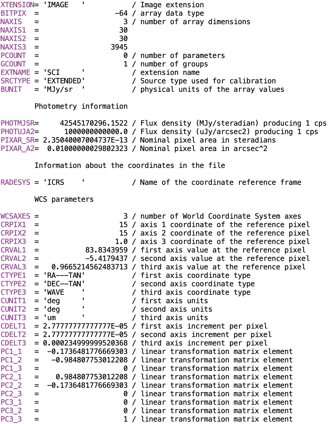
The metadata is composed of two fits headers, a primary header and a header for extension 1 of the data (primary image). We create these headers by making a copy of the header provided by STScI for NIRSpec IFU simulated observations. The primary header contains the information related to the program such as the name of the mission, program, PI, etc. This header is common to all instruments, we replace the relevant information with that from the header created for our ERS program using the pipeline for NIRCam simulations (Canin et al. 2021). In addition, information related to the target and the exposure is replaced manually using the information found in the APT proposal. In the image header, the information relative to the WCS parameters is replaced manually with the coordinates $(\texttt{CRVAL1},\texttt{CRVAL2})=(83.8343959,-5.4179437)$ at the reference point $(\texttt{CRPIX1},\texttt{CRPIX2})=(15,15)$ . An extract of the image header is presented in Fig. 8.

The file corresponding to this simulation can be downloaded at (Canin et al. 2022). The same approach allows to compute the NIRSpec IFU files for the other filters sets (i.e. G235H/F170LP and G395H/F290LP), provided one has the template format for these filters, which is not the case at the time we publish this document.

IV Results

Fig. 4 presents the contents of the $\mathbf{C_{s}}$ cube for two wavelengths, $0.97\mu m$ and $2.87\mu m$ . Fig. 5 presents the spectra of the three $\mathbf{C_{f}}$ cubes extracted in the green circle region in Fig. 6 which presents an image in of the final simulated cube $\mathbf{C_{f}}$ , at $2.12\mu$ m. This cube can be downloaded at this link.

References

Bagnasco et al. (2007) Bagnasco, G., Kolm, M., Ferruit, P., et al. 2007, in Society of Photo-Optical Instrumentation Engineers (SPIE) Conference Series, Vol. 6692, Cryogenic Optical Systems and Instruments XII, ed. J. B. Heaney & L. G. Burriesci, 66920M, doi: 10.1117/12.735602
Berné et al. (2022) Berné, O., Habart, E., Peeters, E., et al. 2022, PASP in prep
Canin et al. (2021) Canin, A., Berné, O., & team, T. P. E. 2021, PDRs4all: Simulation and data reduction of JWST NIRCam imaging of an extended bright source, the Orion Bar. https://arxiv.org/abs/2112.03106
Canin et al. (2022) —. 2022, NIRSpec IFU simulation of the Orion Bar with F100LP/G140H filter, Zenodo, doi: 10.5281/zenodo.5776707
Gardner et al. (2006) Gardner, J. P., Mather, J. C., Clampin, M., et al. 2006, Space Sci. Rev., 123, 485, doi: 10.1007/s11214-006-8315-7
Guilloteau et al. (2020) Guilloteau, C., Oberlin, T., Berné, O., Habart, É., & Dobigeon, N. 2020, AJ, 160, 28, doi: 10.3847/1538-3881/ab9301
Jones et al. (2019) Jones, C., D’Avella, D., Robitaille, T., et al. 2019, spacetelescope/cubeviz: v0.3 - Release v0.3, 0.3.0, Zenodo, doi: 10.5281/zenodo.2616702
Kimble et al. (2008) Kimble, R. A., MacKenty, J. W., O’Connell, R. W., & Townsend, J. A. 2008, in Space Telescopes and Instrumentation 2008: Optical, Infrared, and Millimeter, ed. J. M. O. Jr., M. W. M. de Graauw, & H. A. MacEwen, Vol. 7010, International Society for Optics and Photonics (SPIE), 431 – 442, doi: 10.1117/12.789581
Perrin et al. (2014) Perrin, M. D., Sivaramakrishnan, A., Lajoie, C.-P., et al. 2014, in Society of Photo-Optical Instrumentation Engineers (SPIE) Conference Series, Vol. 9143, Space Telescopes and Instrumentation 2014: Optical, Infrared, and Millimeter Wave, ed. J. Oschmann, Jacobus M., M. Clampin, G. G. Fazio, & H. A. MacEwen, 91433X, doi: 10.1117/12.2056689
Piquéras et al. (2010) Piquéras, L., Legros, E., Pons, A., et al. 2010, in Modeling, Systems Engineering, and Project Management for Astronomy IV, ed. G. Z. Angeli & P. Dierickx, Vol. 7738, International Society for Optics and Photonics (SPIE), 407 – 417, doi: 10.1117/12.856860
Pontoppidan et al. (2016) Pontoppidan, K. M., Pickering, T. E., Laidler, V. G., et al. 2016, in Society of Photo-Optical Instrumentation Engineers (SPIE) Conference Series, Vol. 9910, Observatory Operations: Strategies, Processes, and Systems VI, ed. A. B. Peck, R. L. Seaman, & C. R. Benn, 991016, doi: 10.1117/12.2231768

Appendix A Listings

A.1 Command to calculate the throughputs

⬇

obsmode = { ’instrument’: ’nirspec’,

’mode’: ’ifu’,

’disperser’: ’g140h’,

’filter’: ’f100lp’}

detector = {’readout_pattern’: ’nrsrapid’,

’nint’: 1,

’ngroup’: 5}

conf = {’instrument’: obsmode, ’detector’: detector}

i = pandeia.engine.instrument_factory.InstrumentFactory(config=conf)

pce = i.get_total_eff(tabwave)

A.2 Command to calculate the NIRSpec PSF

⬇

nrs = webbpsf.NIRSpec()

nrs.image_mask = None # No MSA for IFU mode

wl = tabwave[start:end] # Cropped cube

cube = nrs.calc_datacube(wavelengths=wl, fov_pixels=fov_pixels)