An oracle-based framework for robust combinatorial optimization

Enrico Bettiol Thanks: TU Dortmund University {enrico.bettiol@math.tu-dortmund.de} Christoph Buchheim Thanks: TU Dortmund University {christoph.buchheim@math.tu-dortmund.de} Marianna De Santis Thanks: Sapienza University of Rome {marianna.desantis@uniroma1.it} Francesco Rinaldi Thanks: University of Padova {rinaldi@math.unipd.it}

Abstract

We propose a general solution approach for min-max-robust counterparts of combinatorial optimization problems with uncertain linear objectives. We focus on the discrete scenario case, but our approach can be extended to other types of uncertainty sets such as polytopes or ellipsoids. Concerning the underlying certain problem, the algorithm is entirely oracle-based, i.e., our approach only requires a (primal) algorithm for solving the certain problem. It is thus particularly useful in case the underlying problem is hard to solve, or only defined implicitly by a given software addressing the certain case. The idea of our algorithm is to solve the convex relaxation of the robust problem by a simplicial decomposition approach, the main challenge being the non-differentiability of the objective function in the case of discrete or polytopal uncertainty. The resulting dual bounds are then used within a tailored branch-and-bound framework for solving the robust problem to optimality. By a computational evaluation, we show that our method outperforms straightforward linearization approaches on the robust minimum spanning tree problem. Moreover, using the Concorde solver for the certain oracle, our approach computes much better dual bounds for the robust traveling salesman problem in the same amount of time.

Keywords. robust optimization, global optimization, simplicial decomposition

1 Introduction

Robust optimization has become a wide and active research area in the last decades. The aim is to address optimization problems with uncertain data. Unlike the stochastic optimization problem, which usually aims at optimizing expected values, the robust optimization paradigm tries to optimize the worst case. While stochastic optimization requires full knowledge of the probability distributions of all uncertain problem data, robust optimization only asks for a so-called uncertainty sets containing all scenarios that need to be taken into account. While generally leading to computationally easier problems than stochastic optimization, it is well-known that robust counterparts of tractable combinatorial optimization problems usually turn out to be NP-hard for most types of uncertainty sets; see, e.g., [18] or the recent survey [10] and the references therein.

In this paper, we address robust counterparts of general combinatorial optimization problems of the type

\begin{array}[]{l l}\min&c^{\top}x+c_{0}\\[4.30554pt] \textnormal{\,s.t. }&x\in X,\end{array}

(P)

where $X\subseteq\{0,1\}^{n}$ is any set of binary vectors describing the feasible solutions of the problem at hand. The objective function coefficients $(c_{0},c)\in\mathbb{R}^{n+1}$ are considered uncertain. The robust counterpart of (P) is then given by

\begin{array}[]{l l}\min&\max_{(c_{0},c)\in U}\;c^{\top}x+c_{0}\\[4.30554pt] \textnormal{\,s.t. }&x\in X,\end{array}

(R)

where $U\subseteq\mathbb{R}^{n+1}$ is the so-called uncertainty set, collecting all likely scenarios. Note that allowing an uncertain constant $c_{0}$ makes the approach slightly more general, even though the latter is not relevant in the deterministic problem (P). With respect to the considered type of uncertainty set, our approach is rather general, but we will concentrate our exposition on the so-called discrete uncertainty case, where $U$ is given as a finite set. Other classes of uncertainty sets often considered in the literature include polytopal or ellipsoidal sets.

While many approaches devised in the literature consider special classes of combinatorial structures $X$ , our aim is to devise an entirely oracle-based approach. We thus assume that we have at our disposition an algorithm that solves Problem (P), for any given objective $c$ , but we do not pose any restrictions on how this algorithm works. Our approach is thus particularly well-suited in situations where the certain problem is already NP-hard but well-studied, such as, e.g., the traveling salesman problem, or where the underlying problem is not a classical textbook optimization problem, but given by some sophisticated and probably obscure solution software. Our approach does not require any knowledge about the underlying problem.

As mentioned above, robust counterparts are often NP-hard even in cases where the underlying problem (P) is tractable. Consequently, in order to solve (R), it cannot suffice to call the oracle a polynomial number of times. This is even true without assuming P $\neq$ NP [8]. Instead, we propose a branch-and-bound approach, where the main ingredient is the computation of the lower bound given by the straightfoward convex relaxation of (R), namely

\begin{array}[]{l l}\min&\max_{(c_{0},c)\in U}\;c^{\top}x+c_{0}\\[4.30554pt] \textnormal{ s.t. }&x\in\conv(X).\end{array}

(C)

This problem is well-defined and convex, as long as $U$ is any compact set. While ellipsoidal uncertainty leads to a smooth objective in (C), which can be exploited algorithmically [12, 11], the discrete and the polytopal uncertainty cases lead to piecewise linear objective functions, requiring different solution methods.

In our approach, Problem (C) is solved by an inner approximation algorithm; see, e.g., [5] and the references therein. It belongs to the class of Simplicial Decomposition (SD) methods. First introduced by Holloway in [16] and then further studied in [15, 22, 24, 25], SD methods currently represent a standard tool in convex optimization. Our SD method makes use of two different oracles: the first one is an algorithm for solving the convex relaxation over an inner approximation of $\conv(X)$ , being the convex hull of a subset $X^{\prime}$ of $X$ . It is important to notice that such a subroutine implicitly defines the uncertainty set $U$ , while the rest of our algorithm is independent of $U$ . The second oracle is the one described above, which implicitly defines the set $X$ and hence also $\conv(X)$ . Our approach can thus be seen as an oracle-based version of a generalized SD algorithm; see, e.g., [5, 6] for further details about generalized SD. The proposed method indeed performs a two-step optimization process by handling an ever expanding inner approximation of the relaxed feasible set $\conv(X)$ . At a given iteration, the method first builds up a reduced problem (whose feasible set is given by the inner approximation) and solves it by means of the first oracle. It then feeds the second oracle with the information coming from the first step to hopefully generate new extreme points that guarantee a refinement of the inner approximation. If a new point cannot be found, then the solution obtained with the last reduced problem is the optimal one. The way the refinement step is carried out is crucial to guarantee finite convergence of our method in the end.

Dropping rules (i.e., rules that allow to get rid of useless points in the inner approximation) are often used in simplicial decomposition like algorithms to keep the computational cost deriving from the first oracle small enough; see, e.g., [5, 7, 25]. As pointed out in [6], defining suitable dropping rules for a generalized simplicial decomposition, while guaranteeing finite convergence of the method, is a challenging task. We propose a simple dropping rule and analyze it in depth both from a theoretical and a computational point of view.

Some other oracle-based algorithms for robust combinatorial optimization with objective function uncertainty have been devised in the literature. In particular, tailored column generation approaches for dealing with the continuous relaxation of the given combinatorial problem are studied in [9, 17]. When considering Problem (C), those column generation algorithms turn out to be closely related to a Kelly’s cutting plane approach for the problem

\max_{(c_{0},c)\in U}\;\min_{x\in\conv(X)}\;c^{\top}x+c_{0}\;,

which is equivalent to (C) in case of convex $U$ by the minimax theorem. Another interesting approach to handle the relaxation (C) is described in [20], where the author proposes a projected subgradient method that approximately solves the projection problem at each iteration by the classical Frank-Wolfe algorithm. This approach is somehow related to gradient-sliding methods, see, e.g., [21] and the references therein, and hence obviously differs from the one described in this paper.

When aiming at general approaches that do no not exploit specific characteristics of the underlying problem (P), the main alternative to oracle-based algorithms are approaches based on an IP-formulation of (P). For discrete uncertainty, the non-linear objective in (C) can easily be linearized, and this approach can be extended to infinite uncertainty sets $U$ using a dynamic generation of worst-case scenarios, provided that a linear optimization oracle over $U$ is given; see [23] for a general analysis and [14] for an experimental comparison with reformulation-based approaches. The scenario generation method is still applicable when having only a separation algorithm for $\conv(X)$ at hand. In the experimental evaluation presented in this paper, we compare our SD approach to such a separation oracle based approach for the discrete uncertainty case, using CPLEX to solve the resulting integer linear problems.

In the subsequent section, we describe our SD approach in more detail, concentrating on the discrete uncertainty case and with a particular focus on dropping rules. In Section 3, we explain how we embedded this approach into a branch-and-bound framework. An experimental evaluation is presented in Section 4. Section 5 concludes.

2 Computation of lower bounds

The main ingredient in our approach is the computation of the lower bound given by the convex relaxation of the robust counterpart (R). Setting $P:=\conv(X)$ and $f(x):=\max_{(c_{0},c)\in U}c^{\top}x+c_{0}$ , the problem we address is thus given as

\begin{array}[]{l l}\min&f(x)\\[4.30554pt] \textnormal{ s.t. }&x\in P.\end{array}

(CR)

It is easy to see that the objective function $f$ in (CR) is convex for any uncertainty set $U$ , however, it is not necessarily differentiable. E.g., in case of a finite set $U$ , differentiability is guaranteed only in points $\bar{x}$ where the scenario $(c_{0},c)\in U$ maximizing $c^{\top}\bar{x}+c_{0}$ is unique. In the following, we first describe the general idea of the simplicial decomposition approach applied to the potentially non-differentiable problem (CR); see Section 2.1. Afterwards, we investigate a variant of the approach where vertices are dropped in case they are not needed to define the current simplex. This however requires to deal with the issue of cycling; see Section 2.2.

2.1 General approach

We now describe the two oracles that we embed in our SD framework. The first oracle SIM-O essentially minimizes $f$ over a simplex given by the convex hull of a finite set $V\subset\mathbb{R}^{n}$ . Beyond the optimal solution $x^{*}$ , we also need coefficients yielding $x^{*}$ as a convex combination of points in $V$ and a subgradient $c$ of $f$ in $x^{*}$ such that $-c$ belongs to the normal cone of $\conv(V)$ in $x^{*}$ . The existence of such $c$ is a necessary and sufficient condition of optimality for $x^{*}$ .

input : finite subset

V\subset\mathbb{R}^{n}

output :

\alpha^{*}\in\mathbb{R}^{V}_{+}

with

\sum_{v\in V}\alpha^{*}_{v}=1

x^{*}=\sum_{v\in V}\alpha^{*}_{v}v

, and

c^{*}\in\partial f(x^{*})\cap(-\mathcal{N}_{\conv(V)}(x^{*}))

Algorithm 1 SIM-O

The second oracle, namely Oracle LIN-O, is the main oracle defining the underlying problem. It takes as input an objective vector $c$ and returns a minimizer of $\min_{x\in X}c^{\top}x$ , which is the same as solving Problem (P).

input :

c\in\mathbb{R}^{n}

output : optimizer

x^{*}

\min_{x\in X}\;c^{\top}x

Algorithm 2 LIN-O

Using these oracles, Algorithm SD works as follows (see the pseudo-code below): the set $V^{k}$ is initialized as the singleton $\{\hat{x}^{0}\}$ , where $\hat{x}^{0}$ is an arbitrary element of $X$ . Then, we enter a loop. At each iteration $k$ , oracle SIM-O is first called, in order to calculate a minimizer $x^{k}$ of $f$ over $\conv(V^{k})$ and a subgradient

c^{k}\in\partial f(x^{k})\cap(-\mathcal{N}_{\conv(V^{k})}(x^{k}))\;.

Then, oracle LIN-O is called, giving as output a minimizer $\hat{x}^{k}$ of $(c^{k})^{\top}x$ over $x\in X$ . Note that both $x^{k}$ and $\hat{x}^{k}$ belong to $P=\conv(X)$ , but not necessarily to $X$ . From the definition of $\mathcal{N}_{\conv(V^{k})}(x^{k})$ we have that

(c^{k})^{\top}x\geq(c^{k})^{\top}x^{k}\quad\forall\;x\in\conv(V^{k}).

This means that as long as $(c^{k})^{\top}\hat{x}^{k}<(c^{k})^{\top}x^{k}$ we can go further in the minimization of $f$ over $P$ by including the point $\hat{x}^{k}$ in the set $V^{k}$ . Otherwise, if ${c^{k}}^{\top}\hat{x}^{k}\geq{c^{k}}^{\top}x^{k}$ we can stop our algorithm, as $x^{k}$ is a minimizer of $f$ over $P$ and $f(x^{k})$ is a lower bound for Problem (R). See Fig. 1 for an illustration.

given : oracles LIN-O and SIM-O

output : optimizer

x^{*}

of (CR)

compute any

\hat{x}^{0}\in X

by calling LIN-O with arbitrary objective
set

V^{1}=\{\hat{x}^{0}\}

for $k=1,2,\ldots$ do

compute

\alpha^{k},x^{k},c^{k}

by calling SIM-O for the set

V^{k}

compute

\hat{x}^{k}

by calling LIN-O with objective

c^{k}

if $(c^{k})^{\top}\hat{x}^{k}\geq(c^{k})^{\top}x^{k}$ then

STOP:

x^{k}

minimizes

f

over

P

end if

set

V^{k+1}:=V^{k}\cup\{\hat{x}^{k}\}

end for

Algorithm 3 SD

Figure 1: Illustration of Algorithm SD with

X=\{0,1\}^{2}

We claim that Algorithm SD terminates after finitely many iterations with a correct result. For showing this, first observe

Lemma 1.

At every iteration $k$ of Algorithm SD, a lower bound for Problem (CR) is given by $f(x^{k})+(c^{k})^{\top}(\hat{x}^{k}-x^{k})$ .

Proof.

Define $c_{0}:=f(x^{k})-(c^{k})^{\top}x^{k}$ . Since $c^{k}\in\partial f(x^{k})$ , and by the choice of $\hat{x}^{k}$ , we obtain

f(\bar{x})\geq f(x^{k})+(c^{k})^{\top}(\bar{x}-x^{k})=c_{0}+(c^{k})^{\top}\bar{x}\geq c_{0}+\min_{x\in P}\;(c^{k})^{\top}x=c_{0}+(c^{k})^{\top}\hat{x}^{k}

for all $\bar{x}\in P$ , so that $c_{0}+(c^{k})^{\top}\hat{x}^{k}=f(x^{k})+(c^{k})^{\top}(\hat{x}^{k}-x^{k})$ is a lower bound for Problem (CR). ∎

Theorem 1.

Algorithm SD terminates after a finite number of iterations with a correct result.

Proof.

Correctness immediately follows from Lemma 1, since $f(x^{k})$ is clearly an upper bound for Problem (CR) and the algorithm only terminates when $(c^{k})^{\top}\hat{x}^{k}=(c^{k})^{\top}x^{k}$ . So it remains to show finiteness. From the definition of $\mathcal{N}_{\conv(V^{k})}(x^{k})$ we have that

(c^{k})^{\top}x\geq(c^{k})^{\top}x^{k}\quad\forall\;x\in\conv(V^{k}).

This means that in case Algorithm SD does not terminate at iteration $k$ , the point $\hat{x}^{k}\in X$ does not belong to $V^{k}$ , so that $V^{k+1}$ is a strict extension of $V^{k}$ . The result then follows from the finiteness of $X$ . ∎

Note that this proof of convergence relies on our general assumption that $X$ is a finite set and on the fact that we never eliminate vertices of $V^{k}$ . The situation is more complicated when such an elimination is allowed, as discussed in Section 2.2 below.

In the remainder of this subsection, we concentrate on the important special case that $U$ consists of a finite number of scenarios $\{c_{1},c_{2},\ldots,c_{m}\}\subseteq\mathbb{R}^{n+1}$ , where we denote $c_{i}=(\tilde{c}_{i},\bar{c}_{i})$ with the uncertain constant being $\tilde{c}_{i}$ . In this case, the oracle SIM-O can be realized as follows: first note that we essentially need to solve the problem

\min_{x\in\conv(V^{k})}f(x)=\min_{x\in\conv(V^{k})}\max\{\bar{c}_{1}^{\top}x+\tilde{c}_{1},\,\bar{c}_{2}^{\top}x+\tilde{c}_{2},\ldots,\bar{c}_{m}^{\top}x+\tilde{c}_{m}\}.

(1)

In the following, we denote by $x^{k}$ the minimizer of (1), adopting the same notation used within Algorithm SD. As mentioned in [6], having a finite number of scenarios is one of the special cases where the calculation of a subgradient $c^{k}\in\partial f(x^{k})\cap(-\mathcal{N}_{\conv(V^{k})}(x^{k}))$ can be obtained as a byproduct of the solution of (1). For sake of completeness, we report how the subgradient $c^{k}$ is derived. Problem (1) can be rewritten as

\begin{array}[]{l l}\min&z\\[4.30554pt] \textnormal{ s.t. }&\bar{c}_{j}^{\top}x+\tilde{c}_{j}\leq z,\quad j=1,\ldots,m\\[5.16663pt] &x\in\conv(V^{k})\;.\end{array}

(2)

From the optimality conditions of (2), we have that the optimal solution $(x^{k},z^{k})$ , together with the dual optimal variables $\lambda^{k}_{j}$ , satisfies

\begin{array}[]{l r}z^{k}=f(x^{k})=\max\{\bar{c}_{1}^{\top}x^{k}+\tilde{c}_{1},\,\bar{c}_{2}^{\top}x^{k}+\tilde{c}_{2},\ldots,\bar{c}_{m}^{\top}x^{k}+\tilde{c}_{m}\}\\[10.76385pt] x^{k}\in\conv(V^{k}),\;\quad\bar{c}_{j}^{\top}x^{k}+\tilde{c}_{j}\leq z^{k}\qquad j=1,\ldots,m&\mbox{(primal feasibility)}\\[10.76385pt] \displaystyle(x^{k},z^{k})\in\argmin_{x\in\conv(V^{k}),\;z\in\mathbb{R}}\left\{\left(1-\textstyle\sum_{j=1}^{m}\lambda^{k}_{j}\right)z+\textstyle\sum_{j=1}^{m}\lambda^{k}_{j}\bar{c}_{j}^{\top}x\right\}&\mbox{(Lagrangian optimality)}\\[17.22217pt] \lambda_{j}^{k}\geq 0,&\mbox{(dual feasibility)}\\[15.0694pt] \lambda_{j}^{k}=0\quad\mbox{ if }\;\;\bar{c}_{j}^{\top}x^{k}+\tilde{c}_{j}<z^{k}=f(x^{k})\qquad j=1,\ldots,m&\mbox{(complementary slackness)}\end{array}

It follows that $\sum_{j=1}^{m}\lambda^{k}_{j}=1$ and, from Lagrangian optimality, we have

\Big(\sum_{j=1}^{m}\lambda^{k}_{j}\bar{c}_{j}\Big)^{\top}(x-x^{k})\geq 0,\qquad\forall x\in\conv(V^{k}).

(3)

It can be shown (see [4], p.199) that the vector $c^{k}:=\sum_{j=1}^{m}\lambda^{k}_{j}\bar{c}_{j}$ is a subgradient of $f$ at $x^{k}$ , and (3) implies that $-c^{k}$ belongs to the normal cone of $\conv(V^{k})$ at $x^{k}$ , so that we indeed have $c^{k}\in\partial f(x^{k})\cap(-\mathcal{N}_{conv(V^{k})}(x^{k}))$ . Summarizing, when the set $U$ is finite, an oracle SIM-O suited for our purposes can be implemented by any linear programming solver able to address Problem (2), rewritten considering the $\alpha_{v}^{k}$ as variables. In this way, $x^{k}$ is obtained as the convex combination of $\alpha_{v}^{k}$ .

In case of a differentiable function $f$ , the choice of $c^{k}$ is unique. In case of finite $U$ , one may ask the question whether there is some freedom in the choice of $c^{k}$ , which could potentially be exploited in order to find particularly promising search directions. However, it turns out that even in the discrete uncertainty case, the subgradient $c^{k}$ is unique with high probability when the scenarios are chosen (or perturbed) randomly.

Theorem 2.

Assume that all scenarios in $U=\{c_{1},\dots,c_{m}\}$ are perturbed by any continuously distributed random vector in $\mathbb{R}^{m(n+1)}$ with full-dimensional support. Then, with probability one, the set $\partial f(x^{k})\cap(-\mathcal{N}_{\conv(V^{k})}(x^{k}))$ is a singleton in each iteration.

Proof.

By definition, there exist $z^{k}$ and $\alpha^{k}$ such that $(z^{k},x^{k},\alpha^{k})$ is a basic optimal solution of

\begin{array}[]{l l}\min&z\\[4.30554pt] \textnormal{ s.t. }&\bar{c}_{j}^{\top}x+\tilde{c}_{j}\leq z,\quad j=1,\ldots,m\\[5.16663pt] &x=\sum_{v\in V^{k}}\alpha_{v}v\\ &\alpha\geq 0\\ &\sum_{v\in V^{k}}\alpha_{v}=1\;.\end{array}

(4)

Define $A^{=}:=\{v\in V^{k}\mid\alpha^{k}_{v}=0\}$ and $C^{=}:=\{j\in\{1,\dots,m\}\mid\bar{c}_{j}^{\top}x^{k}+\tilde{c}_{j}=z^{k}\}$ . As the feasible set of (4) has dimension $|V^{k}|$ , we have $|C^{=}|+|A^{=}|\geq|V^{k}|$ , and equality holds with probability one. Now $\partial f(x^{k})=\conv\{\bar{c}_{j}\mid j\in C^{=}\}$ has dimension at most $|C^{=}|-1$ and $\mathcal{N}_{\conv(V^{k})}(x^{k})$ has dimension $n-(|V^{k}|-|A^{=}|-1)$ . Consequently, with probability one, the sum of the two dimensions is at most $n$ . Again with probability one, it follows that $\partial f(x^{k})$ and $-\mathcal{N}_{\conv(V^{k})}(x^{k})$ intersect in at most one point. ∎

2.2 Vertex dropping rule

The running time of an iteration of Algorithm SD strongly depends on the size of $V^{k}$ . The overall performance could thus benefit from a dropping rule for elements of $V^{k}$ . A straightforward idea is to eliminate vertices not needed to define the minimizer of $f$ over $V^{k}$ . We thus consider the following modified update rule:

V^{k+1}:=\{v\in V^{k}\mid\alpha^{k}_{v}>0\}\cup\{\hat{x}^{k}\}.

(drop)

In the following, we will refer to Algorithm SD where $V^{k}$ is updated according to (drop) as Algorithm SD-DROP. In case of a non-differentiable function $f$ , Algorithm SD-DROP may cycle, as shown in the following example.

Example 1.

Let us consider the following problem

\begin{array}[]{l l}\min&\max\{x_{1}-x_{2},x_{2}-x_{1}\}\\[4.30554pt] \textnormal{ s.t. }&x_{1}+x_{2}\leq 1\\ &x_{1},x_{2}\geq 0.\end{array}

Starting from $x^{1}={0\choose 0}$ , Algorithm SD-DROP will perform the following iterations:

k=1:

$x^{1}={0\choose 0}$ , $V^{1}=\{x^{1}\}$ , $\alpha^{1}=(1)$ and $\partial f(x^{1})\cap(-\mathcal{N}_{\conv(V^{1})}(x^{1}))=\conv\{{1\choose-1},{-1\choose 1}\}$ .
We choose $c^{1}={1\choose-1}$ . Then $\hat{x}^{1}={0\choose 1}$ , $V^{2}=\{{0\choose 0},{0\choose 1}\}$
k=2:

$x^{2}={0\choose 0}$ , $\alpha^{2}={1\choose 0}$ and $\partial f(x^{2})\cap(-\mathcal{N}_{\conv(V^{2})}(x^{2}))=\conv\{{0\choose 0},{-1\choose 1}\}$ .
We choose $c^{2}={-1\choose 1}$ . Then $\hat{x}^{2}={1\choose 0}$ , $V^{3}=\{{0\choose 0},{1\choose 0}\}$
k=3:

$x^{3}={0\choose 0}$ , $\alpha^{3}={1\choose 0}$ and $\partial f(x^{3})\cap(-\mathcal{N}_{\conv(V^{3})}(x^{3}))=\conv\{{0\choose 0},{1\choose-1}\}$ .
We choose $c^{3}={1\choose-1}$ . Then $\hat{x}^{3}={0\choose 1}$ , $V^{4}=\{{0\choose 0},{0\choose 1}\}$ .

At iteration $k=3$ , we thus get $V^{4}=V^{2}$ and the algorithm cycles. See Fig. 2 for an illustration.

Figure 2: Illustration of Example 1.

Considering this example, two questions may arise. Firstly, the solution $x^{1}$ is actually optimal, so that choosing a better subgradient (namely zero) would have stopped the algorithm immediately. Secondly, the scenarios $(0,1,-1)^{\top}$ and $(0,-1,1)^{\top}$ defining the uncertainty set $U$ contain negative entries. The following example shows that neither of the two features causes cycling:

Example 2.

Let us consider the following problem

\begin{array}[]{l l}\min&\max\{x_{1},x_{2}\}\\[4.30554pt] \textnormal{ s.t. }&x_{1}+x_{2}\geq 1\\ &x_{1},x_{2}\leq 1.\end{array}

Starting from $x^{1}={1\choose 1}$ , Algorithm SD-DROP will perform the following iterations:

k=1:

$x^{1}={1\choose 1}$ , $V^{1}=\{x^{1}\}$ , $\alpha^{1}=(1)$ and $\partial f(x^{1})\cap(-\mathcal{N}_{\conv(V^{1})}(x^{1}))=\conv\{{1\choose 0},{0\choose 1}\}$ .
We choose $c^{1}={1\choose 0}$ . Then $\hat{x}^{1}={0\choose 1}$ , $V^{2}=\{{1\choose 1},{0\choose 1}\}$
k=2:

$x^{2}$ may be ${1\choose 1}$ again, with $\alpha^{2}={1\choose 0}$ , so we eliminate ${0\choose 1}$ , hence $V^{2}=\{{1\choose 1}\}=V^{1}$ .

See Fig. 3 for an illustration.

Figure 3: Illustration of Example 2.

It is easy to see that cycling cannot occur when $f$ is differentiable. In fact, in this case, if $x^{k}$ is not optimal for Problem (CR), we have $f(x^{k+1})<f(x^{k})$ , since $-c^{k}$ is a descent direction. In particular, Algorithm SD-DROP terminates after a finite number of iterations.

For the case of finite $U$ , differentiability is not given, and cycling can occur as seen in the examples above. However, we can still show a weaker result: we will prove that a small random perturbation of the scenario entries can avoid cycling (with probability one). For this, we first need the following observation.

Lemma 2.

Let $L$ be an affine subspace of $\mathbb{R}^{n}$ and assume that $f|_{L}$ , the restriction of $f$ to $L$ , is differentiable in $x\in L$ . Consider $y\in L$ and $c\in\partial f(x)$ with $c^{\top}(y-x)<0$ . Then $y-x$ is a descent direction of $f$ in $x$ .

Proof.

Let $d:=y-x$ . Then $\frac{\partial f}{\partial d}(x)=-\frac{\partial f}{\partial(-d)}(x)$ , since $f|_{L}$ is differentiable in $x$ . From $c\in\partial f(x)$ we obtain $\frac{\partial f}{\partial(-d)}(x)\geq c^{\top}(-d)$ . Hence $\frac{\partial f}{\partial d}(x)\leq c^{\top}d<0$ . ∎

Lemma 3.

Consider an iteration $k$ in which Algorithm SD-DROP does not terminate. Let $L$ be an affine subspace of $\mathbb{R}^{n}$ containing $x^{k}$ such that

(i)

$f|_{L}$ is differentiable in $x^{k}$ ,
(ii)

$\dim(L\cap\aff(V^{k+1}))\geq 1$ ,
(iii)

and $c^{k}$ is not orthogonal to $L\cap\aff(V^{k+1})$ .

Then $f(x^{k+1})<f(x^{k})$ .

Proof.

By (ii), there exists some $y\in L\cap\aff(V^{k+1})$ with $y\neq x^{k}$ . Since $L$ and $\aff(V^{k+1})$ are affine spaces both containing $x^{k}$ , we may choose $y$ such that $(c^{k})^{\top}(y-x^{k})\leq 0$ . By (iii), we may even assume that $(c^{k})^{\top}(y-x^{k})<0$ . Using Lemma 2 and (i), we thus derive that $y-x^{k}$ is a descent direction of $f$ in $x^{k}$ . It thus remains to show that $x^{k}+\varepsilon(y-x^{k})\in\conv(V^{k+1})$ for some $\varepsilon>0$ , which implies that some $\bar{x}\in\conv(V^{k+1})$ has a strictly smaller objective value than $x^{k}$ and hence $f(x^{k+1})\leq f(\bar{x})<f(x^{k})$ .

Since $y\in\aff(V^{k+1})$ , we can write $y=x^{k}+\sum_{v\in\bar{V}^{k}}\gamma_{v}(v-x^{k})+\delta(\hat{x}^{k}-x^{k})$ , where we define $\bar{V}^{k}:=\{v\in V^{k}\mid\alpha^{k}_{v}>0\}$ . As $x^{k}$ belongs to the relative interior of $\conv(\bar{V}^{k})$ , there exists $\bar{\varepsilon}>0$ such that $x^{k}+\sum_{v\in\bar{V}^{k}}\bar{\varepsilon}\gamma_{v}(v-x^{k})\in\conv(\bar{V}^{k})$ . From $(c^{k})^{\top}(y-x^{k})<0$ , $(c^{k})^{\top}\hat{x}^{k}<(c^{k})^{\top}x^{k}$ , and $(c^{k})^{\top}(v-x^{k})=0$ for all $v\in\bar{V}^{k}$ we derive $\delta>0$ . By choosing $\bar{\varepsilon}\leq\tfrac{1}{\delta}$ , we may assume that $x^{k}+\bar{\varepsilon}\delta(\hat{x}^{k}-x^{k})\in\conv(V^{k+1})$ . Altogether, we derive that $x^{k}+\tfrac{1}{2}\bar{\varepsilon}(y-x^{k})\in\conv(V^{k+1})$ . ∎

Theorem 3.

Assume that all scenarios in $U=\{c_{1},\dots,c_{m}\}$ are perturbed by any continuously distributed random vector in $\mathbb{R}^{m(n+1)}$ with full-dimensional support. Then, with probability one, Algorithm SD-DROP terminates after finitely many iterations.

Proof.

Consider any iteration $k$ in which Algorithm SD-DROP does not terminate. Then it suffices to show that $f(x^{k+1})<f(x^{k})$ with probability one. For this, let $L$ be the maximal affine space such that $x^{k}\in L$ and $f|_{L}$ is differentiable in $x^{k}$ . By the definition of $f$ , the epigraph $\epi(f)$ is a polyhedron, and $L$ is obtained by projecting the minimal face of $\epi(f)$ containing $(x^{k},f(x^{k}))$ onto $\mathbb{R}^{n}$ and taking the affine hull of the projection. Thus $L$ is an affine subspace of $\mathbb{R}^{n}$ containing $x^{k}$ , depending continuously on the perturbation of $c_{1},\dots,c_{m}$ . We claim that the conditions (ii) and (iii) of Lemma 3 are satisfied with probability one then, so that the result follows. Indeed, using the same notation as in the proof of Theorem 2, we have $\dim(L)=n-\dim(\partial f(x^{k}))=n-(|C^{=}|-1)=n-(|V^{k}|-|A^{=}|-1)=n-\dim(\aff\bar{V}^{k})$ with probability one, since $|C^{=}|+|A^{=}|=|V^{k}|$ with probability one. Thus, with probability one, we obtain $\dim(L)+\dim(\aff\bar{V}^{k})=n$ and hence $\dim(L)+\dim(\aff V^{k+1})\geq n+1$ . Thus (ii) holds with probability one. For showing (iii), we use again that $\dim(L\cap\aff V^{k+1})\geq 1$ with probability one. This implies that the probability of the fixed vector $c^{k}$ being orthogonal to $L\cap\aff V^{k+1}$ is zero. ∎

Theorem 3 shows that cycling can be avoided by applying small random perturbations to the scenarios $c_{1},\dots,c_{m}$ , e.g., by choosing $(\hat{c}_{j})_{i}\in[(c_{j})_{i}-\varepsilon,(c_{j})_{i}+\varepsilon]$ uniformly at random for some $\varepsilon>0$ , independently for all $j=1,\dots,m$ and $i=0,\dots,n$ . As $X$ is finite, the optimal solution of the perturbed problem (R) will agree with an optimizer of the unperturbed problem if $\varepsilon$ is small enough (even though this is not true for the relaxation (CR)). Note that Theorem 3 requires that also the constant in the objective function is perturbed.

Remark 1.

In practice, the perturbation applied in Theorem 3 is not necessary, because small numerical errors arising in the optimization process will have the same effect. In our experiments described in Section 4, we do not explicitly apply any perturbation.

Note that Theorem 2 also holds when eliminating vertices. In particular, this implies that, when starting from the same set $V^{k}$ , the next subgradient $c^{k}$ is the same with or without elimination (with high probability). However, in a later iteration, the set $V^{k}$ and hence the optimal solution $x^{k}$ may be different in the two cases, and thus also the subgradients. In our experiments, we observed that vertices being eliminated were sometimes re-generated in subsequent iterations.

3 Embedding SD into a branch-and-bound scheme

In order to solve Problem (R) to optimality, we embed Algorithm SD into a branch-and-bound scheme, which we will denote by BB-SD. In this branch-and-bound scheme, we can exploit some specific features of the SD algorithm. Firstly, all binary vertices generated at some node of the branch-and-bound tree can be reused in the child nodes. Indeed, if we branch on fractional variables, each such vertex must be feasible in one of the child nodes, and can thus be inherited. This initial set of vertices enables us to warmstart the SD algorithm at every child node. Moreover, thanks to Lemma 1, every iteration of SD leads to a valid lower bound on the solution of the convex relaxation considered, meaning that early pruning can be performed. In other words, at every node we do not necessarily need to solve the convex relaxation to optimality: the node can be pruned as soon as SD computes a lower bound greater than the current upper bound.

As emphasized above, we assume that Problem (P) can be accessed only by an optimization oracle. Therefore, even when dealing with specific combinatorial problems, we do not exploit any structure to define primal heuristics within BB-SD. Nevertheless, at every node of BB-SD, we easily get an upper bound by evaluating the objective function on all the generated extreme points and taking the minimal value among them.

Having no problem-specific heuristics, we need an enumeration strategy that provides primal solutions quickly. Thus, we adopt a depth first search (DFS). Moreover, the branching rule implemented within BB-SD branches on variables that are fractional in the continuous relaxation, by means of the canonical disjunction. More precisely, we branch on the variable with the fractional part closest to one and produce two child nodes: in the node considered first, we fix the branching variable to $1$ , in the other node we fix it to $0$ . This choice, combined with DFS, typically allows to quickly find integer solutions, which are sparse for many combinatorial problems. Note that all nodes in BB-SD remain feasible. Indeed, regardless of how we select the fractional variable $x_{i}$ to branch on, the oracle must have already returned solutions with both $x_{i}=0$ and $x_{i}=1$ .

4 Numerical results

To test the performance of our algorithm SD and of the branch-and-bound scheme BB-SD, we considered instances of Problem (R) with two different underlying problems: the Spanning Tree problem (Section 4.1) and the Traveling Salesman problem (Section 4.2). The standard models for these problems use an exponential number of constraints that can be separated efficiently. In the case of the Spanning Tree problem, this exponential set of constraints yields a complete linear formulation, while this is not the case for the NP-hard Traveling Salesman problem. For the robust Minimum Spanning Tree Problem, we report a comparison between BB-SD and the MILP solver of CPLEX [3]. For the robust Traveling Salesman Problem, we focus on the continuous relaxations, thus reporting a comparison on the bounds obtained at the root node of the branch-and-bound tree.

In the implementation of SD, for both the robust Minimum Spanning Tree Problem (r-MSTP) and the robust Traveling Salesman Problem (r-TSP), oracle LIN-O is defined according to the underlying problem: for the r-MSTP we implemented the standard Kruskal algorithm [19], a well-known polynomial-time algorithm. For the r-TSP, we used the implementation of the solver Concorde [1]. Since the TSP is NP-hard, the computational times needed to call the linear oracles differ significantly in the two problems, as seen later in the numerical experiments.

Except for the oracle LIN-O, we used exactly the same implementation for both problems. In particular, we applied the same oracle SIM-O for both r-MSTP and r-TSP. Problem (2) is rewritten by expanding the condition $x\in\conv(V^{k})$ . By using the LP formulation (4) and eliminating the $x$ variables, we obtain the following equivalent formulation:

\begin{array}[]{l l}\min&z\\[4.30554pt] \textnormal{ s.t. }&\sum_{v\in V^{k}}\tilde{c}_{j}^{v}\alpha_{v}\leq z,\quad j=1,\ldots,m\\[5.16663pt] &\sum_{v\in V^{k}}\alpha_{v}=1\\[5.16663pt] &\alpha_{v}\geq 0,\quad v\in V^{k},\end{array}

(5)

where $\tilde{c}_{j}^{v}=c_{j}^{\top}v$ , for every $v\in V^{k}$ . Problem (5) is solved with CPLEX. Note that the number of constraints depends on the number of scenarios, and the number of variables corresponds to the cardinality of $V^{k}$ and thus increases at every iteration in our approach SD. The dropping rule implemented in SD-DROP may reduce the size of this problem, thus potentially leading to practical improvements in the running time.

4.1 Spanning Tree Problem

Given an undirected weighted graph $G=(N,E)$ , a minimum spanning tree is a subset of edges that connects all vertices, without any cycles and with the minimum total edge weight. We use the following formulation of the Robust Minimum Spanning Tree problem:

\begin{array}[]{rrcll}\min&\lx@intercol\max_{c\in U}c^{\top}x\hfil\lx@intercol\\[6.45831pt] \textnormal{ s.t.}&\sum_{(u,v)\in E}x_{u,v}&=&|N|-1\\[4.30554pt] &\sum_{u,v\in X}x_{u,v}&\leq&|X|-1&\forall\,\emptyset\neq X\subseteq N\\[4.30554pt] &x&\in&\{0,1\}^{E}\end{array}

(r-MSTP)

The objective function can easily be linearized by introducing a new variable $z\in\mathbb{R}$ and constraints $z\geq c^{\top}x$ for all $c\in U$ . In the above model, the number of inequalities is exponential in the input size, hence we have to use a separation algorithm within CPLEX.

For our experiments, we consider a benchmark of randomly generated instances of r-MSTP. We build complete graphs of five different sizes (from $20$ to $60$ nodes). The nominal costs are real numbers randomly chosen in the interval $[1,2]$ . For each size we randomly generate $10$ different nominal cost vectors. The scenarios $c\in U$ are generated by adding to the vector of nominal costs a random unit vector, multiplied by a scalar factor $\beta$ . We consider three such factors $1$ , $2$ , and $3$ , and generate three different numbers of scenarios (#sc) $10$ , $100$ , and $1000$ . In total, then, we have a benchmark of 450 instances.

In a first experiment, we analyze different dropping rules within algorithm SD. Then, we show how performing a warm start along the branch-and-bound iterations leads to a significant reduction in terms of number of iterations compared to a cold start. Finally, our branch-and-bound method BB-SD is compared to the MILP solver of CPLEX. Within CPLEX, we apply a dynamic separation algorithm using a callback adding lazy constraints, adopting a simple implementation based on the Ford-Fulkerson algorithm.

4.1.1 Comparison of dropping rules

In this section, we focus on the performance of algorithm SD for solving the continuous relaxation of our r-MSTP instances. In particular, we compare the performance of SD implementing three different dropping rules. Since all instances with 10 or 100 scenarios are solved in less than $0.1$ seconds, we only consider the continuous relaxations of instances with $1000$ scenarios, meaning that the evaluation is carried out on $150$ instances. As dropping rules, we implemented the following:

•

d0: meaning that no dropping rule is applied within SD
•

d1: meaning that we update the set $V^{k}$ according to condition (drop) defined in Section 2.2, i.e., we eliminate all vertices $v\in V^{k}$ such that $\alpha_{v}^{k}=0$ at every iteration of SD
•

d2: meaning that we eliminate vertices $v\in V^{k}$ such that $\alpha_{v}^{k}=0$ only if they provide a strict ascent direction, i.e., if $(c^{k})^{\top}(v-x^{k})\geq\varepsilon$ with a fixed threshold $\varepsilon>0$ .

As mentioned before, for each $|N|$ we built $30$ instances, $10$ for each factor $\beta$ . In Table 1, we report the average running times (time) and the average numbers of iterations (#it) for each version of SD; note that the number $n$ of variables in (P) is given by $|E|$ here.

Refer to caption — Figure 4: Comparison between different dropping rules ( $1000$ scenarios).

		d0		d1		d2
$\|N\|$	$\|E\|$	time	#it	time	#it	time	#it
20	190	0.27	69.3	0.30	105.0	0.25	73.1
30	435	0.85	111.1	0.95	184.4	0.73	110.6
40	780	1.72	152.2	2.31	295.2	1.59	155.6
50	1225	2.55	173.6	3.74	353.6	2.44	172.4
60	1770	3.36	208.5	4.65	416.6	3.28	205.5

Table 1: Comparison between different dropping rules (

1000

scenarios).

We further report the performance profiles [13] related to the CPU time and the number of iterations in Fig. 4. We notice that dropping rule d2 allows SD to have slightly better performance in terms of CPU time, despite being not always better with respect to SD with no dropping rule in terms of number of iterations. Indeed, in the MST problem, the linear oracle calls are extremely fast, while most of the computational time is needed to solve the master problem (5). This explains why, although some more iterations are needed, dropping some vertices and hence reducing the size of the master problems can improve the overall performance of the algorithm. On the other hand, it is clear from the results that eliminating all inactive vertices as in Algorithm SD-DROP (rule d1) is not beneficial for SD as both the number of iterations and the CPU time increase.

4.1.2 Warmstart benefits

In the following, we evaluate our branch-and-bound method BB-SD. In particular, we will compare the performance of BB-SD considering both SD with no dropping rule (d0) and SD with dropping rule (d2). The comparison is done on all $450$ instances of r-MST. As mentioned before, for each combination of $|N|$ and #sc, we built $30$ instances, $10$ for each value of the scalar factor $\beta$ . In Table 2, we first compare the performance of BB-SD by considering SD with no dropping rule with and without warmstart (d0 no ws vs d0 with ws). In the table, we report the number of instances solved within the time limit of one hour (#sol), the average running times (time), the average number of nodes (#nodes) and the average number of iterations (#it) for each version of SD. All averages are taken over the instances solved within the time limit. It is clear from the results that the warmstart leads to a considerable decrease in the average number of iterations and consequently a significant decrease in CPU time. The same behavior can be noticed when looking at Table 3, where we compare BB-SD using dropping rule d2 with and without warmstart (d2 no ws vs d2 with ws).

			d0 no ws				d0 with ws
$\|N\|$	$\|E\|$	#sc	#sol	time	#nodes	#it	#sol	time	#nodes	#it
20	190	10	30	1.49	6.72e+2	8.00e+3	30	0.84	6.69e+2	4.23e+3
		100	30	60.03	6.85e+3	1.63e+5	30	33.44	6.87e+3	8.56e+4
		1000	24	476.59	6.74e+3	1.66e+5	27	588.38	1.24e+4	1.78e+5
30	435	10	30	13.12	3.15e+3	5.97e+4	30	7.34	3.52e+3	3.21e+4
		100	25	602.07	3.55e+4	1.15e+5	27	451.05	5.04e+4	8.29e+5
		1000	11	493.33	3.47e+3	8.30e+4	14	642.41	8.64e+3	1.12e+5
40	780	10	30	110.32	1.59e+4	4.10e+5	30	51.77	1.59e+4	1.91e+5
		10	17	764.88	3.24e+4	1.10e+6	19	632.17	5.25e+4	8.65e+5
		10	8	1592.79	7.67e+3	1.78e+5	9	837.77	9.12e+3	9.24e+4
50	1225	10	30	441.38	4.35e+4	1.32e+6	30	201.05	4.40e+4	6.10e+5
		100	10	137.71	7.26e+3	1.53e+5	13	558.02	3.47e+4	5.81e+5
		1000	7	1209.52	3.83e+3	9.81e+4	9	810.38	5.92e+3	6.64e+4
60	1770	10	25	513.71	4.21e+4	1.28e+6	30	575.38	9.81e+4	1.47e+6
		100	9	240.12	9.04e+3	2.09e+5	12	689.81	3.50e+4	5.77e+5
		1000	2	867.80	2.08e+3	5.77e+4	3	1136.77	6.47e+3	7.58e+4

Table 2: Using BB-SD with and without warmstart.

			d2 no ws				d2 with ws
$\|N\|$	$\|E\|$	#sc	#sol	time	#nodes	#it	#sol	time	#nodes	#it
20	190	10	30	1.55	6.75e+2	8.25e+3	30	0.88	6.82e+2	4.39e+3
		100	30	61.11	6.85e+3	1.69e+5	30	34.38	6.88e+3	8.82e+4
		1000	24	480.61	6.74e+3	1.70e+5	27	592.45	1.24e+4	1.82e+5
30	435	10	30	14.62	3.39e+3	6.52e+4	30	7.58	3.52e+3	3.24e+4
		100	25	614.89	3.55e+4	1.16e+6	27	461.70	5.04e+4	8.34e+5
		1000	12	695.62	4.76e+3	1.27e+5	14	576.20	7.51e+3	9.94e+4
40	780	10	30	115.76	1.57e+4	4.10e+5	30	53.22	1.56e+4	1.88e+5
		100	17	776.65	3.21e+4	1.08e+6	18	473.66	3.88e+4	6.37e+5
		1000	7	1266.34	6.69e+3	1.42e+5	9	856.06	9.13e+3	9.26e+4
50	1225	10	30	523.91	4.73e+4	1.44e+6	30	229.78	4.71e+4	6.52e+5
		100	10	143.25	7.26e+3	1.53e+5	13	580.32	3.41e+4	5.75e+5
		1000	7	1194.76	3.83e+3	9.81e+4	9	848.74	5.92e+3	6.64e+4
60	1770	10	25	592.07	4.26e+4	1.29e+6	30	584.95	9.07e+4	1.36e+6
		100	9	249.59	9.04e+3	2.09e+5	12	718.41	3.50e+4	5.77e+5
		1000	2	859.83	2.08e+3	5.77e+4	3	1188.03	6.47e+3	7.58e+4

Table 3: Using BB-SD with and without warmstart, applying dropping rule d2.

In Fig. 5, we further report the performance profiles with respect to the CPU time of the four versions of BB-SD. The versions of BB-SD with no elimination (d0) and with dropping rule d2 show very similar performances. Note that from our results it is clear that the instances become harder with a higher number of scenarios. We can also notice that BB-SD with d2 with ws shows slightly better performances when looking at the hardest instances, namely those with $1000$ scenarios.

4.1.3 Comparison between BB-SD and CPLEX

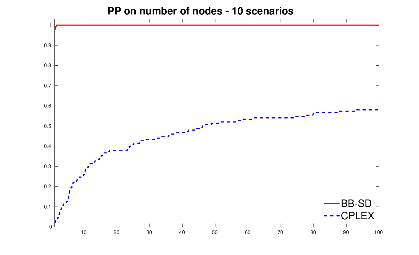
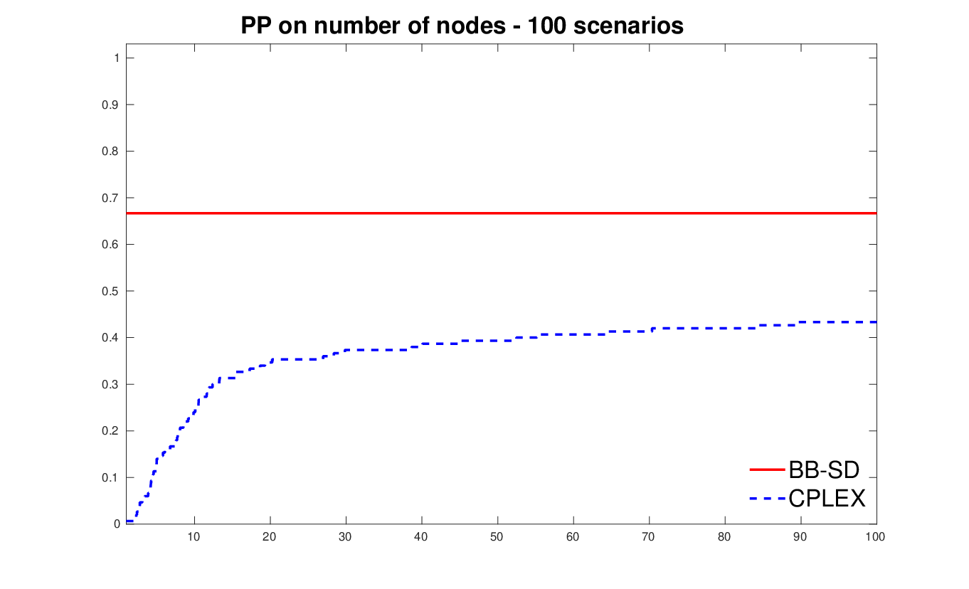
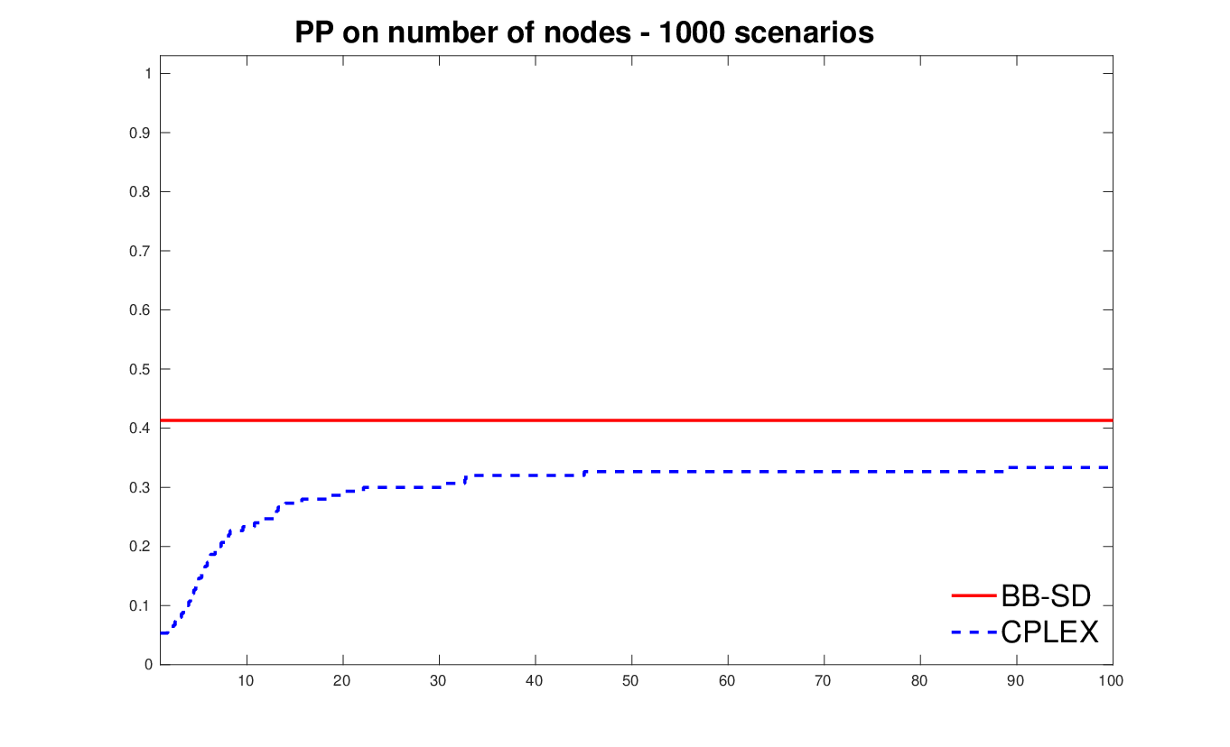
We now compare our branch-and-bound algorithm BB-SD with CPLEX on our r-MSTP instances. As already mentioned, within the MILP solver of CPLEX, we apply a dynamic separation algorithm using a callback adding lazy constraints, adopting a simple implementation based on the Ford-Fulkerson algorithm. The comparison is made with BB-SD implementing the dropping rule d2 and allowing warmstart. In Table 4, we report for each combination of $|N|$ and #sc, the number of instances solved within the time limit of one hour (#sol), the average running times (time) and the average number of nodes (#nodes). We recall that the averages are taken considering the results on $30$ instances each. Performance profiles are presented in Fig. 6.

We can notice that BB-SD strongly ouperforms CPLEX when considering instances with $10$ and $100$ scenarios. As already highlighted before, the higher the number of scenarios, the harder the instances become. Still, also when dealing with instances containing $1000$ scenarios, BB-SD shows better performance with respect to CPLEX. On instances with $10$ scenarios, we see that BB-SD is able to solve all instances within the time limit, while CPLEX fails in $46$ cases. For instances on $100$ scenarios, BB-SD and CPLEX show $50$ and $75$ failures, respectively, while for instances with $1000$ scenarios, BB-SD and CPLEX show $88$ and $95$ failures.

			BB-SD			CPLEX
$\|N\|$	$\|E\|$	#sc	#sol	time	#nodes	#sol	time	#nodes
20	190	10	30	0.88	6.81e+2	30	0.36	2.15e+3
		100	30	34.38	6.88e+3	30	11.85	3.65e+4
		1000	27	592.45	1.24e+4	30	295.54	1.47e+5
30	435	10	30	7.58	3.52e+3	30	39.19	6.80e+4
		100	27	461.70	5.04e+4	27	399.98	7.91e+5
		1000	14	576.20	7.51e+3	17	649.76	2.42e+5
40	780	10	30	53.22	1.56e+4	21	304.25	3.56e+5
		100	18	473.66	3.88e+4	11	897.02	9.29e+5
		1000	9	856.06	9.13e+3	4	1159.91	3.29e+5
50	1225	10	30	229.78	4.71e+4	12	855.83	7.43e+5
		100	13	580.32	3.41e+4	4	685.22	5.17e+5
		1000	9	848.74	5.92e+3	3	3247.92	5.36e+5
60	1770	10	30	584.95	9.07e+4	11	596.26	4.24e+5
		100	12	718.41	3.50e+4	3	1167.98	9.92e+5
		1000	3	1188.03	6.47e+3	1	577.20	8.76e+4

Table 4: Comparison between BB-SD and CPLEX on r-MST instances.

4.2 Traveling Salesman Problem

Given an undirected, complete, and weighted graph $G=(N,E)$ , the Traveling Salesman problem consists in finding a path starting and ending at a given vertex $v\in N$ such that all vertices in the graph are visited exactly once and the sum of the weights of its constituent edges is minimized. Our approach uses the following formulation of the Traveling Salesman problem:

\begin{array}[]{rrcll}\min&\lx@intercol\max_{c\in U}c^{\top}x\hfil\lx@intercol\\[6.45831pt] \textnormal{ s.t.}&\sum_{e\in\delta(i)}x_{e}&=&2&\forall i\in N\\[4.30554pt] &\sum_{e\in\delta(X)}x_{e}&\geq&2&\forall\,\emptyset\neq X\subsetneq N\\[4.30554pt] &x&\in&\{0,1\}^{|E|}\end{array}

(6)

The number of inequalities is again exponential and for CPLEX we use essentially the same separation algorithm as for the Spanning Tree problem; see Section 4.1.

For our tests, we consider 10 instances from the TSPLIB library [2]. For each instance, we generate different scenarios by adding to the nominal costs a random unit vector multiplied by some coefficient. This vector has non-negative components, to avoid negative distances, and the coefficients are $1$ , $2$ and $3$ , as for the r-MST case. We again consider three different numbers of scenarios, namely $10$ , $100$ , and $1000$ , thus producing a benchmark of $90$ instances in total. As mentioned above, we realized the linear oracle by using the solver Concorde. We used the default version and solved each linear problem exactly. In particular, in each linear oracle call an NP-hard problem is solved, so that the time needed by LIN-O is now much larger than the time needed by SIM-O, unlike in the MST case. Therefore, eliminating variables is not effective: it would slightly reduce the time for the linear master problems, while increasing the number of iterations and hence increasing the time to solve the NP-hard oracles. For this reason, for our tests, we only consider SD where no dropping rule is applied.

In the following, we compare the performance of SD applied to solve the continuous relaxation of the instances considered and the performance of CPLEX at the root node. We notice that CPLEX minimizes the non-linear objective function $\max_{c\in U}c^{\top}x$ over the subtour relaxation of the problem, while in our formulation we implicitly optimize the same function over the convex hull of feasible tours, thus obtaining a tighter lower bound. However, our approach needs to solve NP-hard problems to achieve this. It is thus not surprising that the computing time needed by SD to solve the relaxation is often larger than the time needed by CPLEX to solve its weaker relaxation. However, when requiring CPLEX to obtain the same stronger bound, the required computational time increases significantly. In Table 5, we show the results for the TSP instances. For every instance and every number of scenarios, we report the average bound and computing time obtained by SD (SD root node) and by CPLEX (CPLEX root node) to solve the continuous relaxation. In the last column, we report the time needed by CPLEX to obtain the same bound as the SD bound (CPLEX – SD bound). The table shows that, on average, the SD bound is much stronger than the subtour relaxation bound, but it is obtained in a longer time. Furthermore, the time needed by CPLEX to reach the same bound as SD is often much larger than the SD time and in one case the time limit of one hour was reached.

instance	#sc	SD root node		CPLEX		CPLEX
				root node		SD bound
		bound	time	bound	time	time
brazil58	10	46031.5	2.09	41982.9	0.03	1.77
	100	48086.6	12.35	43722.6	0.21	9.75
	1000	49278.8	19.09	44810.6	2.68	256.33
dantzig42	10	1158.0	1.59	1093.1	0.02	0.26
	100	1203.6	0.97	1143.7	0.17	0.99
	1000	1230.9	6.92	1166.3	3.50	15.33
fri26	10	1622.8	0.45	1550.9	0.01	0.09
	100	1691.7	1.32	1624.7	0.07	0.39
	1000	1721.6	1.44	1663.8	0.64	2.75
gr120	10	9801.5	15.96	9564.9	0.16	203.93
	100	9977.8	68.51	9759.4	1.03	672.07
	1000	10131.3	68.74	9886.2	18.34	$>3600.00$
gr17	10	3911.2	0.28	3623.6	0.01	0.04
	100	4053.9	0.57	3676.5	0.02	0.19
	1000	4248.6	0.73	3925.4	0.16	1.94
gr21	10	4928.4	0.22	4903.8	0.01	0.01
	100	5138.5	0.22	5104.6	0.03	0.15
	1000	5301.1	0.23	5277.2	0.24	0.76
gr24	10	2202.9	0.30	2153.9	0.01	0.04
	100	2272.6	0.55	2251.5	0.04	0.16
	1000	2359.8	1.76	2318.3	0.37	1.52
gr48	10	7642.8	0.92	7417.6	0.02	0.43
	100	7907.4	6.38	7668.2	0.14	3.10
	1000	8034.1	8.38	7789.8	1.57	31.01
hk48	10	18545.0	0.55	17895.9	0.02	0.40
	100	18889.0	1.50	18377.3	0.14	2.18
	1000	19190.6	6.74	18854.7	1.63	21.43
swiss42	10	2051.0	1.71	1970.7	0.03	0.50
	100	2128.4	1.41	2064.1	0.16	1.25
	1000	2185.3	9.20	2117.2	2.13	19.31

Table 5: Average results for r-TSP, continuous relaxations.

5 Conclusion

We presented an algorithm for the exact solution of strictly robust counterparts of combinatorial optimization problems, entirely based on a linear optimization oracle for the underlying problem. Concentrating on the discrete scenario case, our experimental evaluation shows that the approach is competitive both in case the underlying problem is very easy to solve, as in the MST case, and in case it is a hard problem, as in the TSP case. In particular, in the latter case, we have seen that solving the underlying problem to optimality can be beneficial even when it is NP-hard: in the same amount of time, our approach produces much better dual bounds than CPLEX based on a linearized IP formulation of the problem, using the standard subtour formulation.

We emphasize again that our approach is not restricted to the case of discrete uncertainty. However, the oracle SIM-O must be adapted when considering other classes of uncertainty sets. In case of ellipsoidal uncertainty, SIM-O turns out to be a second-order cone program. As mentioned above, since $f$ is a smooth function in this case, cycling is not possible even if the most aggressive dropping rule (drop) is used. For the case of polyhedral uncertainty, SIM-O can again be realized as a linear program, and the statement of Theorem 3 holds analogously.

The investigation of other generalizations of our approach is left as future work. In particular, it may be interesting to extend it to more general classes of uncertain objective functions, e.g., of the form $c^{\top}g(x)$ , where a convex function $g\colon\mathbb{R}^{n}\to\mathbb{R}^{m}$ is given and the coefficients $c\in\mathbb{R}^{m}_{+}$ are uncertain. In this case, the function $f$ decribing the worst case over all scenarios is still a convex function, and it suffices to adapt the oracle SIM-O.

References

[1] Concorde TSP solver. https://www.math.uwaterloo.ca/tsp/concorde/index.html.
[2] TSPLIB. http://comopt.ifi.uni-heidelberg.de/software/TSPLIB95.
cpl [2021] IBM ILOG CPLEX Optimizer, 2021.
https://www.ibm.com/it-it/analytics/cplex-optimizer.
Bertsekas [2009] Dimitri P. Bertsekas. Convex Optimization Theory. Athena Scientific, Belmont, MA, 2009.
Bertsekas [2015] Dimitri P. Bertsekas. Convex Optimization Algorithms. Athena Scientific, Belmont, MA, 2015.
Bertsekas and Yu [2011] Dimitri P. Bertsekas and Huizhen Yu. A unifying polyhedral approximation framework for convex optimization. SIAM Journal on Optimization, 21(1):333–360, 2011.
Bettiol et al. [2020] Enrico Bettiol, Lucas Létocart, Francesco Rinaldi, and Emiliano Traversi. A conjugate direction based simplicial decomposition framework for solving a specific class of dense convex quadratic programs. Computational Optimization and Applications, 75(2):321–360, 2020.
Buchheim [2020] Christoph Buchheim. A note on the nonexistence of oracle-polynomial algorithms for robust combinatorial optimization. Discrete Applied Mathematics, 285:591–593, 2020.
Buchheim and Kurtz [2017] Christoph Buchheim and Jannis Kurtz. Min–max–min robust combinatorial optimization. Mathematical Programming, 163(1-2):1–23, 2017.
Buchheim and Kurtz [2018] Christoph Buchheim and Jannis Kurtz. Robust combinatorial optimization under convex and discrete cost uncertainty. EURO Journal on Computational Optimization, 6(3):211–238, 2018.
Buchheim and Santis [2019] Christoph Buchheim and Marianna De Santis. An active set algorithm for robust combinatorial optimization based on separation oracles. Mathematical Programming Computation, 11(4):755–789, 2019.
Buchheim et al. [2018] Christoph Buchheim, Marianna De Santis, Francesco Rinaldi, and Long Trieu. A Frank-Wolfe based branch-and-bound algorithm for mean-risk optimization. Journal of Global Optimization, 70(3):625–644, 2018.
Dolan and Moré [2002] Elizabeth D Dolan and Jorge J Moré. Benchmarking optimization software with performance profiles. Mathematical Programming, 91:201–213, 2002.
Fischetti and Monaci [2012] Matteo Fischetti and Michele Monaci. Cutting plane versus compact formulations for uncertain (integer) linear programs. Mathematical Programming Computation, pages 1–35, 2012.
Hearn et al. [1987] Donald W Hearn, S Lawphongpanich, and Jose A Ventura. Restricted simplicial decomposition: Computation and extensions. In Computation Mathematical Programming, pages 99–118. Springer, 1987.
Holloway [1974] Charles A Holloway. An extension of the frank and wolfe method of feasible directions. Mathematical Programming, 6(1):14–27, 1974.
Kämmerling and Kurtz [2020] Nicolas Kämmerling and Jannis Kurtz. Oracle-based algorithms for binary two-stage robust optimization. Computational Optimization and Applications, 77(2):539–569, 2020.
Kouvelis and Yu [1996] Panos Kouvelis and Gang Yu. Robust Discrete Optimization and Its Applications. Springer, 1996.
Kruskal [1956] Joseph B Kruskal. On the shortest spanning subtree of a graph and the traveling salesman problem. Proceedings of the American Mathematical Society, 7(1):48–50, 1956.
Kurtz [2021] Jannis Kurtz. New complexity results and algorithms for min-max-min robust combinatorial optimization. arXiv:2106.03107, 2021.
Lan [2020] Guanghui Lan. First-order and Stochastic Optimization Methods for Machine Learning. Springer Nature, 2020.
Larsson and Patriksson [1992] Torbjörn Larsson and Michael Patriksson. Simplicial decomposition with disaggregated representation for the traffic assignment problem. Transportation Science, 26(1):4–17, 1992.
Mutapcic and Boyd [2009] Almir Mutapcic and Stephen Boyd. Cutting-set methods for robust convex optimization with pessimizing oracles. Optimization Methods & Software, 24(3):381–406, 2009.
Ventura and Hearn [1993] Jose A Ventura and Donald W Hearn. Restricted simplicial decomposition for convex constrained problems. Mathematical Programming, 59(1):71–85, 1993.
Von Hohenbalken [1977] Balder Von Hohenbalken. Simplicial decomposition in nonlinear programming algorithms. Mathematical Programming, 13(1):49–68, 1977.