Unified gravity at local scales
Abstract
We explore the shifted model with as a distinguishing physical parameter for the study of constraints at local scales. The corresponding dynamics confronted with different geodesics (null and non-null) along with its conformal analogue is investigated. For null geodesics, we discuss the light deflection angle, whereas for non-null geodesics under the weak field limit, we investigate the perihelion advance of the Mercury orbit in Schwarzschild background, respectively. The extent of an additional force, appearing for non-null geodesics, depends on . Such phenomenological investigations allow us to strictly constrain to be approximately with a difference of unity in orders at galactic and planetary scales and seems to provide a unique at local scales. Further, at late cosmic time, we analyse the constraint on via the bare scalar self-interaction Einstein frame potential to provide a null test of dark energy. We constrain the deviation parameter, to which is in a close agreement with the results obtained through various observations in the Jordan frame by several authors. Our results suggest that the present form of model is suitable for the alternate explanation of dark matter-like effects at local scales, whereas at large scales the deviations grow higher and must be addressed in terms of the accelerated background.
pacs
98.80.-k, 95.36.+x, 95.35.+d, 98.80.Jk.I Introduction
Precision cosmology is imperfect without the precise physical observations of systems at different scales. For precise observations, the physical system must be completely known. Unfortunately, the major portion of our observable universe is not completely known to us in the Einstein’s General Relativity (GR) framework. Also, the Einstein’s gravity theory with positive cosmological constant () based on GR supported by observations still can not be regarded as an ultimate gravity theory because of the recent stronger than before Planck’s observation of an accelerating universe ( having the shifted from -1) and its inability to reconcile with the quantum theory completely and also more importantly, the fundamental properties of dark sector (dark energy and cold dark matter) is still unknown besides its distribution. Thus, the observational evidences at different redshifts nurture the concept of modified gravity theory instead of the Einstein’s physical gravity theory of GR with (positive) and cold dark matter (CDM) b1; b2; b3; b4; b5; b6; b7; b8; b08. Actually, the investigation of deviation in the Einstein’s GR theory has become an active area of research under the study of precision concordance cosmology. Therefore, it is the need of precision concordance cosmology to opt for an alternative theory of gravity.
Brans and Dicke first explored the scalar-tensor approach of gravity theory as an alternative to the Einstein-Hilbert (E-H) gravity theory b9 and thereafter H. A. Buchdahl, A. A. Starobinsky and others carried out the study of higher order Lagrangian or non-linear Lagrangian for exploring the cosmic evolution and also for the phenomenological explanation of the major observational issues at different cosmological redshifts of the universe b9; b09; b10; b11; b12; b13; b14; b15; b16; b17; b18; b19; b20; b21; b22; b23; b24; b25; b26; b27; b28; b29; b30; b31; b32; b032. The main implicit powers of the alternate gravity theory can be understand in two ways, on one hand it can address dark sector (dark matter and dark energy) with the different particulate degrees of freedom (see b20) and on the other hand it can precisely address the deviation in the existing gravity theory i.e. Einstein’s GR theory, which at present is very active nowadays in literatures b45; b35; b33; b34; b80. Such alternate gravity theory may also provide a possible way to study the unified theory of dark matter and dark energy b033 .
In this direction, motivated by the dynamical modelling of massive test masses in gravity model by Bhmeret al. b36 and also by our recently investigated power-law model at low redshifts b33; b34; b35 and by others b37; b38; b39; b40 for the clustered dark matter explanation, we further analyse here the precise and strict phenomenological constraints on the model parameter in . That is, we investigate here the constraints corresponding to different geodesics (null and non-null) along with its conformal analogue at the galactic and planetary scales under an idealistic consideration with the modified potential explored in b38; b39; b40. Moreover, our recent combined analysis of light deflection profiles via rotation curves for typical spiral massive galaxies may in principle also diagnose the present model from the other profile of standard dark matter model of galaxy (say Pseudo-isothermal model) in terms of lensing angle b34. With such motivations and also from the motivation drawn from the physical form of deviation introduced in model by Bhmer et al. b36, we look for as a distinguishing parameter for investigating the precise constraints through the study of motions of test masses under the stable orbits in different geodesics (null and non-null) along with its conformal analogue. Although such power-law modification was initially carried out for the study of early-time cosmic evolution, late-time cosmic evolution and also for the galactic dynamic explanation b41; b42; b43 and b36; b37; b38; b39; b40.
From the phenomenological point of view, it seems that formulation have spaces for the explanation of most abundant dark sector of the energy budget of our universe with the standard matter. From the mathematical point of view and motivated by the earlier Jordan-Brans-Dicke Lagrangian b9, the action formulation can be recast into the scalar-tensor form so that one can clearly see the appearance of an extra scalar degree of freedom (scalar fields) which occupy the spaces of dark sectors and unlike some gravity theories in which we have an ad hoc scalar fields b44. Such an extra scalar degree of freedom has non-minimal coupling with the spacetime geometry. Thus, in alternate gravity theories, gravitational interaction can also be mediated via the scalar degrees of freedom (scalaron) together with the spacetime metric tensor (). formulation has also two characteristic length scales, of which one is the Schwarzschild length scale and the other is the characteristic length scale which has an advantage to provide a screening mechanism b45 corresponding to the extra force in high density environments.
For investigating the physical observable effects of such extra scalar degrees of freedom alone (scalaron as scalar field particle), it is preferred in literature that extra scalar degree of freedom should be coupled minimally with the Einstein-Hilbert spacetime geometry () in the action integral so that we can trace its dynamical influence via solving the second order field equations instead of fourth order field equations. This can be possible through the conformal analysis of spacetime metric tensor b44. Thus, we have two gravity actions before and after the conformal transformation i.e., Jordan frame (because the dynamical equations resembles the Jordan-Brans-Dicke gravity theory) and conformal Einstien frame (because the dynamical equations resembles with the Einstein-Hilbert gravity theory). Also, pertaining to the physical observations at different scales, which frame one should prefer is still under debate and several research works have been reported from the early investigations b46; b47; b48; b49; b50; b51, till recent analyses b52; b53; b54; b55; b56; b57; b58. Hence, the well known issue in literature regarding the choice of true physical frame is actually a long standing i.e. which spacetime metric tensor among the conformally related ( or ) should one may choose for representing the geometry of spacetime pertaining to the physical observations. Some scientists claim that both frames are equivalent whereas others claim opposite ( in references b55; b56; b57; b58). The issue can only be settled down through the physical observations of the system.
Several authors had explored this issue before without any firm discussions regarding the most profound physical observations confronted with different geodesics (null and non-null) along with its conformal analogue under the shifted () Einstein-Hilbert theory at local scales. Thus, along with discussing the conformally related different geodesics, we also explore the nature of an additional force in terms of model parameter and further envisage the shifted parameter () as a distinguishing tool for the study of motions at different geodesics to impose the strict constraints on the model via observations.
We also acquired the motivation to explore the bare effects of modification at different scales. Like, from the important analysis to the limit to GR in theory of gravity by G. J. Olmo b59, from the study of model constraints at different scale by W. Hu and I. Sawicki b27, from the recent and early investigation of the Yukawa-like potential in theory b60; b61, from the study of power-law gravity theory b37; b38; b39; b40, from the recent investigation of an uncertainty in the GR prediction for the Mercury orbit under the current (MESSENGER) and planned (the European-Japanese BepiColombo) missions b62; b63; b64; b65; b66, from the analysis of Yukawa type potential in the Schwarzschild-like background for perihelion precession of planets to address the gauge bosons as a possible candidate of fuzzy dark matterb066 and from the relativistic effects and dark matter in the Solar system through the observations of planets and spacecraft b067.
In the present work, we study the deviations in GR in the form (with being the dimensionless physical observable quantity) and instead of investigating the Yukawa-like correction potential as others did b60; b61, we explore the bare modified effects in the form of for different observations without any versions of dark sector. Such form can be modelled in the gravity framework. Also, since physical observations of the system is confronted with different geodesics, we obtain its conformal analogue and investigate the precise deviations at different scales. For instance, we phenomenologically study the geodesics (null and non-null) along with its conformal analogue at local scales under an idealistic considerations and obtain the strict constraints on at galactic and planetary scales, respectively. Such constraints are strict in the sense that for orbital motions at local scales, can be physically represented as with known b36. Further, we explore the extent and nature of an additional force on the test mass due to the shifted modification parameterized by . Next, we analyse the late-time cosmic constraint via the bare potential of Einstein-frame to provide a null test of dark energy, which is also investigated by S. Capozziello under different cosmic observations b77 in jordan frame. The work is followed by the general discussion of conformally transformed gravity action and their field equations. The present paper is organised in different sections as follows. In Section (II), we mathematically discuss the Jordan and conformal Einstein frames dynamical field equations. In Section (III), we discuss the parametrization for geodesics and phenomenologically investigate the null geodesics for the conformally related light deflection angles due to massive spiral galaxies as lens. In Section (IV), we discuss the non-null geodesics and investigate its Newtonian limit for the explanation of additional force in theory. Further, we explore it phenomenologically for the conformally related orbital precession of planet (Mercury) at the solar system scale and analyse and diagnose the tight constraint via specifying as . Next, we discuss the cosmic late-time constraint on the in Section (V) and end with the discussion and concluding remarks of results on the constraints in Section (VI).
Throughout the paper, we follow the signature of the spacetime metric as (, +, +, +) and indices (or ) = (0, 1, 2, 3).
II gravity and conformally related field equations
Lovelock theorem suggests possible modifcation to the gravity theory. According to which, Einstein’s gravity theory of GR is unique theory of gravity, if we demand b67: (i) the metric tensor () is the only field (ii) invariance under diffeomorphism (iii) the equation of motion is second order and (iv) to work with four dimensions.
Any violation of one of these assumptions will provide an alternative or modified gravity theory.
gravity theory focus on the metric tensor and equations of motion.The metric tensor
() is not the only field (but also scalar field) and also the equations of motions are not second order (but becomes forth-order) in gravity theory.
Consider the 4-dimensional action integral having the gravity Lagrangian density possessing some generic function of the Ricci scalar with the usual standard matter action in units of c==1 as,
| (1) |
where is the determinant of the metric tensor , is the Einstein’s gravitational constant with the Newtonian gravitational constant, and is the action of the standard matter part with matter field . We can also write the gravity Lagrangian density of (1) similar to the Jordan-Brans-Dicke gravity theory as,
| (2) |
where with and .
In the action written in the form equation (2), we can see that the extra scalar degrees of freedom in the form of is non-minimally coupled with the geometry () and has the similar form observed in the Jordan-Brans-Dicke gravity action. One can also explore (1) in Helmholtz-Jordan frame and obtainwith the same action which have non-vanishing second derivative. We can perform conformal rescaling of the spacetime metric in order to explore further the dynamics of the extra scalar degrees of freedom.
Therefore, following the well established mathematical procedure of conformal transformation of scalar-tensor theory b44, the conformal map from the four dimensional spacetime manifold with metric to the four dimensional spacetime manifold but with metric i.e.,
| (3) |
along with
| (4) |
whose second term vanishes when (4) is used in the action integral by following the Gauss’ theorem of total derivative which transforms the equation (2) as,
| (5) |
where
| (6) |
is the scalar potential term written in parametric form for general model which has non-vanishing
second derivative and .
Here, instead of considering a new parametric
scalar field11
1
The linear canonical action with minimally coupled
scalar field is obtained by defining a new scalar field with
,
we workout with the action (5) in its simplest form and explore its
field equations.
The field equations in this frame are obtained by varying (5) w.r.t the metric tensor () and the scalar field () which are given as b68,
| (7) |
and
| (8) |
Now, one can obtain the field equations by transforming equations (7) and (8) back to without tilde notation i.e. in the Jordan frame as b68,
| (9) |
where
| (10) |
and
| (11) |
Hence, we get the conformally related equations.
Thus, one can mathematically transform set of equations between the two versions of frame with or . But their physical equivalence is still under debate b47; b48; b49; b52; b53; b54; b55; b56; b57; b58
and can be settled down through the observations. We wish to obtain the precise constraints through conformal analysis that suits the physical observations in both frames.
Therefore, we investigate the null and non-null geodesic equations at the local scales. We then explore the light deflection angle due to a typical massive galaxies and also the perihelion advance of the planet like Mercury’s orbit in the shifted model with parameter . Further, we study the late-time cosmic constraints on .
III conformal investigation of geodesics and phenomenology for null geodesics
The conformal transformation generalizes the spacetime metric according to the form of (see equation 3). Here, we investigate the geodesic equation in different ways i.e., under the re-parametrization and under the conformal analysis for addressing the null and non null dynamics. We express its conformally shifted parameter with new parameter () instead of using tilde notations. The statement can be understood as the action is re-parametrization invariant, so it is possible to express the geodesics (which is a geometrical entity) with different parameter, say . For instance, the geodesics equations in terms of proper time can be written for the material particle following the curve () as,
| (12) |
In terms of new parameter , we can express (12) as,
| (13) |
Thus, we get the generalized equation for geodesics ().
The affine or non-affine nature of the new assigned parameter can be traced if it is expressible in terms of the old parameter () as or vice versa can also be possible. So, on switching from to , if and has a linear relation, then only we can recover the original geodesics equations (12). Such parameters in GR literature can be assigned as affine parameters.
Now, if represents the curves in , then under equation (3), the Levi-Civita connections in have the following relation with the Levi-Civita connections in as,
| (14) |
Thus, the geodesic equation now gets conformally transformed under equation (3) and is given as,
| (15) |
From this equation, it becomes clear that if represents the geodesics in , then it may not be a geodesic in . Therefore, for the curve in , the parameter must also be conformally shifted.
It is interesting that equation (15) resembles the generalized geodesic equation (13) but under the conformal transformation and hence it is conformally modified geodesics in theory. The nature of its parameter in terms of conformal shifting or affine (non-affine) as argued for equation (13) can be traced for the null and non-null cases. For the null case, the last term of conformally modified geodesic equation (15) vanishes because . So, equation (15) gets reduced to
| (16) |
Further, to trace the conformal shift (or affine nature) of parameter , we reduce the equation (16) as argued for equation (13).
Therefore, we re-parameterize the equation (16) under , with as a new parameter (conformally shifted) and is given as,
| (17) |
We find that, if the parameter has a conformal relation with as,
| (18) |
then under such conformal relation, equation (17) becomes,
| (19) |
Thus, the geodesics of particles having zero rest mass remain unaffected for the conformally related spacetime equation (3) in theory. Hence, can be regarded as a conformally shifted (or an affine) parameter. Therefore, the conformally transformed spacetime metric exhibits the same causal structure.
Now, for the phenomenological study of null geodesics, we explore the light deflection angle due to a typical spiral massive galaxies. Following b38; b39; b40, let us consider a static Schwarzschild-like metric element outside the source under the four-dimensional spacetime with as,
| (20) |
where the quantities and act like the functions of weak gravitational potential. The actual form of potentials can be determined via solving the vacuum field equations for the function of Ricci scalar () entering in the generalized Einstein-Hilbert gravity action integral.
Now, to calculate the deflection angle in gravity theory, we must know the complete form of metric element or the form of the effective potential. For the investigation of light deflection angle, we closely follow the references b38; b39. It becomes clear from the discussions of b38 that the formal expression for the total deflection angle of light ray (following null geodesics) in gravity theory must remain the same under the weak field limit of Schwarzschild-like metric. The components of Schwarzschild-like metric critically depend upon the expression chosen for curvature part of the Lagrangian.
Thus, for the physically motivated metric element like equation (20) with obeying the power-law in Ricci curvature scalar ( dimensionless constant), we have an explicit expression for the modified effective gravitational potential in the weak field limit with explored first by Capozziello et al., and further investigated by other authors b37; b39; b40 as well for the study of galactic dynamics. For a point-like baryonic mass in background, the effective gravitational potential is given as,
| (22) |
with
| (23) |
where and is the scaling length, whose appearance is natural in gravity theory due to the Noether’s symmetry (seeb45 and references therein). is new parameter related with the shifted model parameter () as in equation (23) b39. It is clear from the equations (22) and (23) that for we have , and the Newtonian limit is recovered.
Furthermore, we have also recently investigated the constraint on the model parameter to be from the combined study of flatness profile of rotation curves and the corresponding deflection angle profile in the halo of scalaron cloud (instead of dark matter) surrounding the typical massive galaxies b23; b24. Behmer et al., investigated the small value of the power-law model b36 valid for the discussion at local scale. Therefore, it is possible to rewrite equation (22) in the narrowest range of and for the study of local scale dynamics. Since, in the narrowest range, the order of and have approximately one-to-one relation (see Fig. 1).
Thus, we can express equation (22) in terms of model parameter with smaller values as,
| (24) |
Clearly, for , we recover the GR Lagrangian along with its relevant Newtonian potential.
The profile of with respect to can be understood from Fig. (2).
Thus, we prefer to work with the small values of model parameter .
Now, under the conformal transformation (obtained through equations (20) and (21)), the effective potential (equation (24)) can be conformally shifted on making use of equation (3) in the weak field limit and is written as,
| (25) |
Further, withequation (3) under the footnote (1) for with as a weight constant having dimension of Ricci Scalar (), we have,
| (26) |
Now, under the weak field limit, with normalized to unity, we have
| (27) |
Thus, equation (25) can be rewritten on using equation (27) as,
| (28) |
The light deflection angle for a spherically symmetric lens (a typical massive spiral galaxy) with the massive point-like effective potential (equation (24)), in background is given as b38,
| (29) |
where, is a two-dimensional impact parameter, is the Newtonian gravitational constant ( kpc km2 sec-2 ), is fundamental scaling parameter in theory apart from the Schwarzschild length scale b45 and is galaxy mass in solar mass unit. The famous classical result of light deflection angle is recovered for .
For the conformally transformed effective lens potential (equation (28)), the light deflection angle will be,
| (30) |
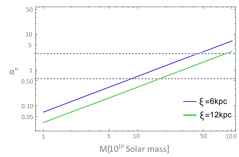
The profile of net deflection angles according to the equations (29) and (30) is plotted in Fig. 3 and Fig. 4.
Thus, it becomes clear by the profile of net light deflection angles from different figures (3 and 4) to choose the narrow values of () for conformal equivalence.
The small (about ) profile of is also recently confirmed from our study of galactic dynamics b33; b34.
Therefore, for the physical interpretation, we explore the small values of for the light deflection angles due to the typical massive spiral galaxy system acting as a point-like lens and trace it via the known physical observations of lensing data for few galaxies culled from b69 and references therein.
For instance, the quantitative analysis of the net modified deflection angle can be explored by considering the case of an object having solar mass unit (like a typical massive spiral galaxy) in the galactic halo (halo of scalaron cloud due to the background) acting as a weak lens for the light rays coming from the source star positioned in the external galaxy, like the Magellanic clouds.
Fig. 5 shows the profile of deflection angles plotted with smaller value of for different typical massive galaxies acting as a point source. The observed profile of deflection angle for the galaxies b69 is in agreement with the explored model without dark matter, so the conformally related deflection angles seem to be physically equivalent for b34; b69.
We have also plotted in Fig.6 the deflection angles for typical massive galaxies in GR.
As an important point to draw attention here is that the extent of can also be probed directly via the study of orbital motion of neutral hydrogen clouds (as a test particle) in stable orbits far from the visible profile of typical spiral galaxies with taking km/s b36.
IV conformal non-null geodesics analysis and phenomenology for perihelion shift
Because of the uncertainty in the GR predicted result of Mercury’s orbit b62; b63; b64; b65 as well as the upcoming probes b66, motivate us to study the Mercury’s orbit in theory in order to investigate the bare effect of deviation () at the planetary scale, i.e. .
Earlier investigation for the present case was done with Yukawa-like potential in theory b38. Unlike deflection of light, here the case is that an object (test mass) never gets out to infinity where the spacetime metric is asymptotically Minkowskian. Hence, for the study of conformal non-null geodesics, we start from equation (15). Under this case, the last term of equation (15) does not vanish for the non-relativistic material particles having non-zero rest mass and so it is not further possible to reduce the equation (15) to the original one (12) by different conformal relations like equation (18). Thus, equation (15) suggests that under the conformally related spacetime (equation (3)), the non-null trajectories experiences an extra force for unit test mass. This extra force can be the carrier of a new particle. In gravity theory, this new particle will be the scalar field particle called scalaron (see reference b72).
Let us investigate the non-relativistic case of equation (15) for the material particle (non-zero rest mass) tracing the curve . For mathematical convenience, we normalize its last term, b73. Thus, equation (15) can be re-written as,
| (31) |
In the non-relativistic limit with (space coordinates) one should get the Newtonian equation with the conventional gravitational force b73. Therefore, equation (31) has the following form,
| (32) |
So, under the non-relativistic Newtonian limit, equation (32) becomes,
| (33) |
Now, if is the conventional (or standard) force of gravity, then under the conformal transformation of spacetime metric (equation (3)), we have an additional force on the unit test mass,
| (34) |
where is the general conformal factor of the theory.
Clearly, the extent of such extra force will depend upon the extent of model parameter () and vanishes for . Also, in contrast to the Newtonian gravitational force, it die off in strength slowly as,
| (35) |
where, , and is the Ricci scalar curvature corresponding to the metric equations (20) with (24). It becomes clear from equation (35) that the suppression of such extra force depends on the constrained values of which from the observations in high-density regions is usually much small.
It is concluded from the non-vanishing value of given as,
| (36) |
that outside the source, value of Ricci curvature scalar depends on the model parameter and vanish for in GR theory and hence the corresponding force also vanish. As it is well known that a deviation from the Newtonian force is responsible to a perihelion advancement of Mercury’s orbit (explained observationally by Einstein’s gravity theory). Therefore, any modification in the Einstein’s GR theory must be much smaller for interpreting phenomenologically the present case.
Now, for the phenomenological study of conformal non-null geodesics under an idealized consideration of system, we explore the time-like orbit of Mercury at the Solar system scale.
We simplify the problem in theory by using the corresponding symmetries and write the modified gravity Lagrangian following equation (20) as,
| (37) |
where is given by equation (22) and the dot denotes differentiation w.r.t the proper time ().
The and equations following from this Lagrangian are given by using Euler’s Lagrangian formalism as,
| (38) |
and
| (39) |
where, and are constants. The equation can be simplified for material particle with as,
| (40) |
| (41) |
Now, on defining a new variable as,
| (42) |
and
| (43) |
In contrast to the Newtonian classical equation of motion b73, we have
| (45) |
we can rewrite the modified relativistic equation (44) as,
| (46) |
where, with as total energy of the system. We observe that the relativistic correction factor (the last term which is responsible for the advancement of perihelion motion of a planet) is also enhanced by modification. Therefore, the deviated (i.e., ) modifications must be smaller in order not to violate the GR result but possible probe the uncertainty found if any by different current running projects and to have an agreement with the observation. Such modification may be compatible for explaining an uncertainty in the GR prediction under the current (MESSENGER)b65 and planned (the European-Japanese BepiColombo) b66 missions.
If we express with as a Schwarzschild length in units of and as a modified Schwarzschild length, then (46) can be written as,
| (47) |
Clearly, for , we recover the GR differential equation of motion and hence, the shift in perihelion
can be obtained via the standard perturbation approach to the Newtonian solution b73.
Now, to determine the shift in perihelion, we solve equation (47) by equating it to zero, since for perihelion and aphelion is fixed. Actually, this will suggest us different positions. Since equation (47) is a cubic equation, so has and as its three different solutions or roots. But the semi-classical observed problem has bounded solution between perihelion and aphelion . Thus, among the three solutions, one solution must be an unphysical. Therefore, if we assume that as an unphysical solution, then we must eliminate it from equation (47) for the study of bounded motion.
From equation (47), it is possible to replace the R.H.S. with the three roots viz., , and as,
| (48) |
Under the assumption of bounded motion, , equation (48) can be rewritten as,
| (49) |
To eliminate the assumed unphysical solution i.e., from equation (49), we must impose a boundary condition on the three solutions.
Since has the dimension of inverse of length and has the dimension of length. Because and are basically considered as two roots of equation (45), so represents the inverse length of major axis b73 and if is positive then must be a large in contrast to modified Schwarzschild length . So, the plausible boundary condition can be constructed as,
| (50) |
Now, equation (51) become,
| (54) |
Further, equation (54) can be solved to give,
| (55) |
The twice of the left hand side of the equation (56) suggests the angle between successive perihelion. The perihelion shift can be computed as,
| (57) |
Thus, the required perihelion shift in gravity theory is,
| (58) |
The last factor of above equation can be classically given from the values of perihelion and aphelion in terms of semi-major axis and eccentricity b73. So, we can rewrite equation (58) under the observed bounded motion as,
| (59) |
where is the semi-major axis, is the eccentricity of the orbit which for a planet like Mercury are available from the observations and is the speed of light. The last factor in equation (59) in numerator indicates that deviation , which arises due to modification in Einstein gravity under , contributes to the perihelion shift within the permissible limit and therefore must be much smaller. Thus, the effect of such modification may probe the uncertainty in GR result as suggested after different missions b62; b63; b64; b65; b66.
We investigate equation (59) for with the values of m and for Mercury precession about the massive Sun, kg and m3/(kg-sec-2). The data is culled from NASA’s Solar System Bodies b74. With these values we get, radian per revolution or per revolution. As, the periodic time of Mercury around the Sun is Earth-days so that it makes revolution per year, or revolutions in one century. Therefore, the advance of the perihelion of Mercury in 1 century is seconds of arc. Thus, the GR result is fully recovered.
The relativistic conformal shift of the perihelion of Mercury orbit can be written (following equation (26) and (27)) as,
| (60) |
The profile of perihelion shift according to the equations (59) and (60) is plotted in Fig. 7 and Fig. 8 for different values of model parameter .
It becomes clear from Fig. 7 that the perihelion shifts ( and ) vary largely w.r.t the small deviation in the model parameter and also not observationally consistent with . But, from Fig. 8, it is clear that for the perihelion shift approximately attains an observable constant value for and .
As a further interesting fact, we also look for the number of revolutions corresponding to the age of our Solar System. For instance, for the degree shift of the orbit, the time taken will be centuries. Now, for 360 degrees, the required time is millions of years (or years). Obviously, this is not very much at cosmological time scale. In about billion years (during which Sun, Earth and other planets form) before the present epoch, the number of revolutions the axis of Mercury has gone through is !
According to Fig. 8, the perihelion shift can be successfully explained for . Such constraint can be directly probed via specifying the model parameter with the orbital velocity of Mercury ( km/s) as . Contrasting with the constraints explored by Zakharov et al., ( ) and Clifton ( ) b37; b037, the explored constraint is different from them and corresponds to the extra force which drops off as . Such relativistic effects is likely to be detectable by different probes as discussed by Will in reference b66. It in also in close approximation with the parameterized post-Newtonian (PPN) estimates.
V Realization of late-time cosmic constraints via bare self-interaction potential
The recent (2018) Planck Collaboration b1; b2 has measured the Equation of State parameter (EoS) , which motivates us to explore an alternative theory of gravity and also because of the serious issues with the classical cosmological constant with b3. Actually, the case of positive cosmological constant (also interpreted as vacuum energy density) can be viewed in two different perspectives till 1998 (its smallness) and after 1998 (its coincidence with present average matter density of the universe). At present, the common view that at the background level there is nothing but a cosmological constant of positive nature and an alternative gravity theory may work at large scales because of the observations demanding the EoS not exactly equal to . We investigate the present model in this connection and explore the constraint via the vacuum solution of the theory with bare conformal potential.
To see the extent of power-law curvature scalar in Jordan frame fitted with the cosmic observational data, Capozziello et al., explored the encouraging results with SNIa and WMAP data and constrained the cosmic viable shifted power-law model parameter, to be approximately -0.6 or 0.4 b77.
Now, to realize the observed late-time cosmic constraint on the shifted model parameter in the conformal Einstein frame, we argue that it is the form of bare curvature scalar potential (equation (6)) that provides the current cosmic acceleration. So, accordingly we can write the observed dark energy parameter (positive Cosmological constant) as b76; b75; b72; b27,
| (61) |
Here is the observed dark energy parameter and is the weight constant of our model which we assign here to be the background mass scale and may represents the critical density or vacuum energy density in the universe today b27. During the late-times saturates (or dilutes) to (cosmic coincidence). Such coincidence can be seen as problematic only if one starts assuming that one could be present with equal probability in any of the periods of the cosmic evolution. But this is definitely not the case b3; b27.
Before exploring (61) under above discussion, we study the extremum condition on the Einstein frame bare potential and obtain the bound on the model parameter . Because it is the bare potential which decides the extremum conditions for the effective potential (i.e., including non-relativistic matter fields) under a suitably chosen function in Einstein frame b35. On using equations (3) and (6) and the Footnote , we have
| (62) |
Clearly, for the minima of effective potential, we must have and . For , the extremum conditions are satisfied as
| (63) |
| (64) |
Therefore, on further simplifying equation (61) with small , we get
| (65) |
Clearly, for , the contribution vanishes and now we have to add by hand a classical cosmological constant in GR geometric action for interpreting present cosmic acceleration.
Now, because of the observed late-time cosmic coincidence, , we get from equation (65)
| (66) |
A small discrepancy in the value of in contrast to b77 may be attributed to the very small discrepancy in the exactness of the equality of and b3. Thus, it seems that in an alternative gravity theories, an approximate ratio of the order of one of the present comparable energy densities is replaced by the necessity to constrain phenomenologically the model parameter corresponding to the dark sectors with an appropriate strength to fit the observational data. Clearly, this is a simple analysis which could be used to constrain the shifted model parameter with the realization of its consistency in different conformal frames.
In this way, different direct evidences from the observations at different scales can precisely constrain the shifted model parameter along with its conformal analogue and it is also realized that can acts as a diagnostic tool to distinguish the two frames and also to provide the precise observational constraints via the combined analysis.
VI Summary and Discussions
Let us then recapitulate the present work briefly. The study of precision cosmology is not possible in GR frame work until we completely know the physical system, but it provides a way to model the deviations in Einstein-Hilbert GR action. Deviations from Einstein GR theory are indeed predicted mostly in various extra-dimensional theories. Contrasting alternatives to Einstein GR are actually useful to understand precisely which features of the theory have been tested in a particular experiment, and also to suggest new experiments probing different features. Such study can be modelled in the gravity framework. Therefore, we study the deviations in GR in the form with being the dimensionless physical observable quantity. We focus on the study of null and non-null geodesics at local scales and explore it under conformal theory. Our discussion shows that conformal transformation of spacetime metric () leaves the null geodesic unchanged (Section III). On the other hand, the effect of such transformation for non-null geodesics produces an additional force on the unit test mass which can be traced under the Newtonian limit (see equation (33) or (34)). We discuss the extent of this additional force in Schwarzschild background and investigate its relativistic effect on the perihelion advance of Mercury orbit by obtaining the expressions for the conformally related orbital precession of Mercury. We also explore some features of the model for small deviations in Figs. (1), (2) and (3), whereas in Figs. (4), (5) and (8) we investigate the physical observations of the system confronted with different geodesics along with its conformal analogue and explore the precise deviations at different scales. The main motivation to explore the deviation in the narrowest value comes from the recent combined investigation of galactic dynamics for the power-law model b33; b34; b36 as well as from b27; b37.
The extra force can be screened in the high density environment as it directly depends on with (see equation (35)) and the observational results can be traced with smaller (Fig. 8). Such deviation can be envisaged as a distinguishing factor since can be specified as as well as also for the conformal investigations of different frames under different physical observations at local scale.
The phenomenological study of different geodesics, light deflection angle for null geodesics and perihelion advance of mercury orbit for non-null geodesics (under an idealistic consideration22 2 It is often stated in literature that the relativistic perihelion advance of Mercury is really only a test of the vacuum Schwarzschild solution, as the general relativistic effects can be derived simply from such metrics. along with its conformal analogue at local scales imposes the strict constraints on to be approximately with a difference of unity in order at galactic and planetary scales respectively (see Figs. 4, 5 and 8). Such constraints are strict in the sense that for orbital motions at local scales, can be physically represented as with known through observations. Our recent analysis of lensing profile of galaxies with for the dark matter model may also, in principle, diagnose the present model from the other galactic standard dark matter model (pseudo-isothermal sphere model etc.). The analysis of perihelion advance of mercury orbit as contrast to other authors b37; b037; b74 shows the new constraints within bare framework to be about . Here, we do not consider the frame-dragging effect on the metric. Since, different missions (surveys) have reported an uncertainty in the GR result for the Mercury orbit b62; b63; b64; b65; b66; b74, so gravity theory may be a potential candidate in this regard. Thus, the present model preserves the same form for the explanation of local scale dynamics including the planetary scales and hence an unique at local scale.
We further analyse the constraint on the deviation parameter, via using the bare scalar self-interaction potential to provide a null test of dark energy. In this direction, we discuss the Einstein frame potential and explore the cosmic late-time constraint on the model parameter to be which is a close agreement with the encouraging results explored in Jordan frame by Capozziello et al. b77. Our analysis provides a powerful tool to obtain the precise constraints on the shifted parameter modelled in gravity at different scales.
Such smaller values for are also consistent with cosmological constraints coming from primordial nucleosynthesis b27; b78; b79.
Currently all operating projects for the detection of gravitational waves, including LIGO, Virgo and LISA are based on geodesic deviation equation, so we will also extend this work in future for the study of binary systems and gravitational wave (GW) analysis and will look for the physical quantity for to directly diagnose the model with GW data in order to investigate uncertainty in the Einstein’s GR theory.
The present status of the custered (DM) and unclustered (DE) dark sector hypothesis and the modified gravity alternatives, deduce that there is a lack of definitive convincing arguments in favour of any of the two concepts or particular theories. Basically, all the gravity models have some successful predictions but also problematic comparisons with some observations and experiments. Therefore, it seems that new observations are necessary, especially on the scale of stars and planetary systems.
As an important comment, because of the highly different values of the shifted parameter of model at different scales (basically at local scale and at late-time cosmic scales), it may not be a suitable model in its present form to study the unified approach to dark matter, dark energy and inflation. The possible investigation of precise modification in this direction (at early time epoch) is also explored by the authors b80. Although, the investigated model seems to be consistent for the study of clustered dark matter like dynamics at local scales and therefore would bridge the gap among the gravitational anomalies ranging from stellar to galactic scales. In this way, different direct evidence from the observations at different scales can precisely constrain the shifted model parameter along with its conformal analogue. Our findings are also in an close agreement with the recently explored values by us at galactic scales and also seems to provide a new phenomenological constraint for the study of perihelion advance of Mercury orbit as it differs from the values explored by different authors.
Acknowledgments
Authors thank IUCAA, Pune, for providing the facilities with which a part of the present work was completed under the associateship programme. VKS also thanks Swagat S. Mishra, B. K. Yadav and A. K. Sharma for fruitful discussions. He thanks Varun Sahni for several comments and support during visits to IUCAA.
References
- (1) N. Aghanim, Y. Akrami, et al., Planck 2018 results, Astron. Astrophys., 641, A6, (2020).
- (2) A. G. Riess et al., (SUPERNOVA SEARCH TEAM collaboration), Astrophys. J. 116, 1009 (1998); B. Schmidt et al., Astrophys. J. 507, 46 (1998); S. Perlmutter et al., Astrophys. J. 517, 565 (1999); D. N. Spergel et al., (WMAP Observations), Astrophys. J. Suppl. 148, 175 (2003).
- (3) T. Padmanabhan, Phys. Rept. 380, 235 (2003) ; R. R. Caldwell and M. Kamionkowski, Annu. Rev. Nucl. Part. Sci., 59, 397, (2009); S. Weinberg, Rev. Mod. Phys. 61, 1 (1989).
- (4) P. Salucci, Astron. and Astrophys. Rev. 124, 27 (2019).
- (5) V. C. Rubin, W. K. Ford, N. Thonnard, Astrophys. J. 238, 471 (1980); V. C. Rubin, D. Burstein, W. K. Ford, and N. Thonnard, Astrophys. J. 289, 81 (1985).
- (6) R. H. Sanders, The Dark Matter Problem: A Historical Perspective (Cambridge University Press, Cambridge, 2010).
- (7) D. Clowe et al., Astrophys. J. 648 L109 (2006).
- (8) S. H. Oh et al., AJ 142, 1 (2011); W. J. G. de Blok, arXiv:0910.3538v1 [astro-ph.CO] (2009).
- (9) Joshua D. Simon et al., xx xxx, xx (2019), arXiv:1903.04742v1 [astro-ph.CO] (2019).
- (10) C. Brans, and R.H. Dicke, Phys. Rev. 124, 925,(1961).
- (11) H. A. Buchdahl, Mon. Not. R. Astron. Soc. 150, 1 (1970).
- (12) A. A. Starobinsky, Phys. Lett. B 91, 99 (1980); A.A. Starobinsky, JETP Lett. 86, 157 (2007).
- (13) M. Milgrom, Astrophys. J. 270, 365 (1983).
- (14) H. Motohashi, A.A. Starobinsky, J. Yokoyama, Int. J. Mod. Phys. D 20 (8), 1347 (2011).
- (15) S. Nojiri, and S. D. Odintsov, TSPU Bulletin N 8 (110), 7-9 (2011).
- (16) T. Clifton et al., Physics Reports 513, 1-3 (2012).
- (17) D. Langlois, Int. J. Mod. Phys. D 28, 05 (2019).
- (18) Christian Arnold, Matteo Leo, and Baojiu Li, Nature 3, 945 (2019).
- (19) N. Israel and J. Moffat, Galaxies 6, 41 (2018).
- (20) T. Kobayashi, and P. G. Ferreira, Phys. Rev. D 97, 121301(R) (2018).
- (21) S. Nojiri, S. D. Odintsov, V. K. Oikonomou, Physics Reports 692, 1-104 (2017).
- (22) T. Katsuragawa and S. Matsuzaki, Phys. Rev. D 95, 044040 (2017).
- (23) T. Katsuragawa and S. Matsuzaki, Phys. Rev. D 97, 064037; Phys. Rev. D 97 (12), 129902 (2018).
- (24) S. S. Mishra, V. Sahni, and Y. Shtanov, JCAP 06, 045 (2017).
- (25) S. Capozziello, M. De Laurentis, G. Lambiase, Phys. Lett. B 715, 1 (2012).
- (26) S. Capozziello and V. Faraoni, Beyond Einstein Gravity: A Survey of Gravitational Theories for Cosmology and Astrophysics (Springer, New York 2011).
- (27) J. A. R. Cembranos, Phys. Rev. Lett. 102 (14), 141301 (2009).
- (28) S. Capozziello, V. F. Cardone and A. Troisi, Mon. Not. Roy. Astron. Soc. 375, 1423 (2007).
- (29) W. Hu, I. Sawicki, Phys. Rev. D 76, 064004 (2007).
- (30) Y. Sobouti, Astron. Astrophys. 464, 921 (2007).
- (31) J. R. Brownstein, J. W. Moffat, Mon. Not. Roy. Astron. Soc. 382, 1 (2007).
- (32) V. Sahni, A. Starobinsky, Int. J. Mod. Phys. D 15, 2105 (2006).
- (33) G. J. Olmo, Phys. Rev. Lett. 95 (26), 261102 (2005).
- (34) S. M. Carroll et al, Phys. Rev. D 70, 043528 (2004).
- (35) Y. Shtanov, arXiv:2105.02662v1 [hep-ph], (2021).
- (36) S. S. Mishra, V. Sahni Eur. Phys. J. C. 81 7, 625 (2021).
- (37) V. K. Sharma, B. K. Yadav, and M. M. Verma, Eur. Phys. J. C 80, 619 (2020).
- (38) V. K. Sharma, B. K. Yadav, and M. M. Verma, Eur. Phys. J. C 81, 109 (2021).
- (39) B. K. Yadav and M. M. Verma, JCAP 10, 052 (2019).
- (40) C. G. Boehmer, T. Harko, and F. S. N. Lobo, Astropart. Phys. 29, 386 (2008).
- (41) A. F. Zakharov et al., Phys. Rev. D 74, 107101 (2006).
- (42) T. Clifton, Class. Quantum Grav. 23, 7445 (2006).
- (43) S. Capozziello, V. F. Cardone, and A. Troisi, Phys. Rev. D 73, 104019 (2006).
- (44) S. Capozziello, V. F. Cardone, and A. Troisi, Mon. Not. Roy. Astron. Soc. 375, 1423 (2007).
- (45) C. F. Martins and P. Salucci, Mon. Not. Roy. Astron. Soc. 381, 1103 (2007).
- (46) V. Muller, H.J. Schmidt, A. A. Starobinsky, Class. Quant. Grav. 7, 1163 (1990).
- (47) S. Capozziello, V. F. Cardone, S. Carloni, A. Troisi, Int. J. Mod. Phys. D 12, 1969 (2003).
- (48) H. Motohashi, Phys. Rev. D 91, 064016 (2015).
- (49) Y. Fujii and K. I. Maeda, The Scalar-Tensor Theory of Gravitation, (Cambridge University Press, 2003).
- (50) S. Capozziello et al., JCAP 06, 044 (2017); Ann. Phys. (Berlin) 524, 545 (2012).
- (51) C. M. Will, Liv. Rev. Rel. 4, 4 (2001).
- (52) Y. M. Cho, Class. Quantum Grav. 14, 2963 (1997).
- (53) G. Magnano and L. Sokolowski, Phys. Rev. D 50, 5039 (1994).
- (54) V. Faraoni and E. Gunzig, Int. J. Theor. Phys. 38, 217 (1999).
- (55) M. Roshan, F. Shojai, Phys. Rev. D 80, 043508 (2009).
- (56) J. D. Barrow and K. Maeda, Nucl. Phys. B 341, 294 (1990).
- (57) E. Elizalde, S. Nojiri, and S. D. Odintsov, Phys. Rev. D 70, 043539 (2004).
- (58) G. Cognola, et al., Phys. Rev. D 77, 046009 (2008).
- (59) S. Capozziello et al., Found. Phys. 39, 1161 (2009).
- (60) S. Capozziello, P. M. Moruno, C. Rubanoa, Phys. Lett. B 689, 117 (2010).
- (61) N. Deruelle and M. Sasaki; Cosmology, Quantum Vacuum and Zeta Functions, 137 (2011) (Conference paper).
- (62) S. Bahamonde et al., Phys. Lett. B 766, 225 (2017).
- (63) M. Rinaldi, Eur. Phys. J. Plus 133, 408 (2018).
- (64) G. J. Olmo, Phys. Rev. D 75, 023511 (2007).
- (65) M. De. Laurentis, I. De Martino, and R. Lazkoz, Phys. Rev. D 97, 104068 (2018).
- (66) I. De Martino, R. Lazkoz, and M. De. Laurentis, Phys. Rev. D 97, 104067 (2018).
- (67) R. S. Park et al., Astron. J 153, 121 (2017).
- (68) L. Iorio, Planetary and Space Science 55, 1290 (2007).
- (69) B. Sun, Z. Cao, and L. Shao, Phys. Rev. D 100, 084030 (2019).
- (70) A. Genova et al., Nature Communication 9, 289 (2018).
- (71) C. M. Will, Phys. Rev. Lett. 120, 191101 (2018).
- (72) T. K. Poddar, S. Mohanty, and S. Jana, Eur. Phys. J. C 81, 286 (2021).
- (73) E. V. Pitjeva and N. P. Pitjev, Mon. Not. R. Astron. Soc. 432, 3431 (2013).
- (74) D. Lovelock, J. Math. Phys. 12, 498 (1971).
- (75) G. J. Olmo and W. Komp, arXiv:gr-qc/0403092v2 (2004).
- (76) M. C. Campigotto et al., JCAP 06, 057 (2017).
- (77) T. P. Sotiriou and V. Faraoni, Rev. Mod. Phys. 82 (2010).
- (78) C. W. Misner, S. Thorne, and J. A. Wheeler, Gravitation (W. H. Freeman and Co., NY, 1973).
- (79) https://solarsystem.nasa.gov; G. G. Nyambuya, Mon. Not. R. Astron. Soc. 403, 1381 (2010).
- (80) X. Zhang, W. Zhao, H. Huang, and Y. F. Cai, Phys. Rev. D 93, 124003 (2016).
- (81) T. Liu, X. Zhang, W. Zhao, Phys. Lett. B 777, 286 (2018).
- (82) S. Capozziello, et al., Int. J. Mod. Phys. D 12, 10 (2003).
- (83) T. Clifton and J. D. Barrow, Phys. Rev. D 72, 103005 (2005).
- (84) S. Nojiri, S. Odintsov, and V. Oikonomou, Class. Quant. Grav. 34, 245012 (2017).
- (85) A. K. Sharma and M. M. Verma, accepted in Astrophys. J. (2021).