Dynamical Lee–Yang zeros for continuous-time and discrete-time stochastic processes
Abstract
We describe classical stochastic processes by using dynamical Lee–Yang zeros. The system is in contact with external leads and the time evolution is described by the two-state classical master equation. The cumulant generating function is written in a factorized form and the current distribution is characterized by the dynamical Lee–Yang zeros. We show that a continuous distribution of zeros is obtained by discretizing the time variable. When the transition probability is a periodically oscillating function of time, the distribution of zeros splits into many parts. We study the geometric property of the current by comparing the result with that of the adiabatic approximation. We also use the Floquet–Magnus expansion in the continuous-time case to study dynamical effects on the current at the fast-driving regime.
I Introduction
Understanding statistical fluctuations of current is one of the main objectives in nonequilibrium physics. When the system is coupled to multiple reservoirs, we observe a current through the system. The fluctuation theorem tells us how the underlying symmetry of the system is reflected to the current distribution ECM; GC; Crooks.
In the long-time limit, the system settles down to a stationary behavior irrespective of the choice of the initial condition. Full counting statistics describes distributions of transferred charges through the system GC; LL; LLL; BN; SU. The generating function can be treated as an analog of the partition function in equilibrium statistical mechanics.
The analytic properties of the partition function can be described by the Lee–Yang zeros YL; LY; Fisher. The partition function is a positive quantity and goes to zero only when we set the parameters to unphysical values. The only exception is when the system has a phase transition. It involves a breakdown of the analyticity and can be described by the distribution of the zeros.
A similar behavior is also expected to hold in the generating function of the full counting statistics. Previous studies found that the generating function is described by the dynamical Lee–Yang zeros AI; IA; FG; UEUA; HFG; SMY16; BMPGF; SMY17. We note that the Lee–Yang zeros are useful not only in the presence of the phase transitions but also for general systems. By knowing the distribution of zeros, we can obtain the complete information of the system. Any statistical quantities are represented by zeros. It was shown in quantum systems WL; PZWCDL and in classical stochastic systems BMPGF that the Lee–Yang zeros are not artificial mathematical objects but are directly related to the experimental observables.
Zeros of the generating function can be clearly understood when the number of events is finite, or countably infinite. For a stochastic process described by the probability distribution , the generating function is defined as
| (1) |
When the positive integer parameter is finite, the generating function, written as
| (2) |
is completely characterized by a set of zeros . Each represents a point where the generating function goes to zero in complex plane of . Statistical quantities calculated from the generating function are represented by using the zeros.
The number of zeros becomes large as the number of events increases. However, previous studies found that the number of zeros in stochastic systems described by the two-state classical master equation is given by a small finite value IA; FG; HFG; BMPGF. This property is totally different from the original Lee–Yang theory where many zeros are accumulated to form a continuous distribution in a complex plane in the thermodynamic limit. To find a similar behavior in stochastic systems, we need to find a controllable parameter that determines the number of zeros.
A different interesting problem is the situation when the system is driven periodically. Then, the transition-rate matrix in the master equation is time dependent. When we treat the system by the adiabatic approximation, the generating function is defined at each time and the zeros oscillate as a function of time. However, they do not represent the zeros of the global generating function. It would be an interesting problem to clarify how to describe the periodically driven systems by the dynamical Lee–Yang zeros.
In this paper, we study distributions of the dynamical Lee–Yang zeros by using the two-state classical master equation in several situations. We show that the number of zeros is controllable by discretizing the time variable. Then, we can find a nontrivial distribution of zeros in the long-time limit. To study periodically driven systems, we use the adiabatic approximation in the slow-driving regime Thouless; SN and the Floquet–Magnus expansion in the fast-driving regime Magnus; BCOR.
The organization of the paper is as follows. In Sec. II, we treat the continuous-time master equation to reproduce known results on the dynamical Lee–Yang zeros. The analysis is extended to the discrete-time master equation to obtain a nontrivial distribution of zeros in Sec. III. Then, we study a periodically driven system from an adiabatic picture in Sec. IV. We also study the continuous-time system with a high frequency in Sec. V. Section VI is devoted to summary.
II Continuous-time process

When we pursue an analogy between the current generating function for stochastic processes and the partition function in statistical mechanics, it is reasonable to study the long-time behavior of the stochastic processes. The time evolution of the probability distribution is generally given by the master equation under the assumption that the process is Markovian. To make the discussion concrete, we treat the system depicted in Fig. 1. The system takes two states (“empty”) and (“filled”), and we observe flows among left and right leads. When the transition-rate matrix in the master equation is time independent, the dynamical Lee-Yang zeros were obtained in previous studies IA; FG; HFG; BMPGF. In this section, we summarize the basic definitions and notations, and reproduce the known results together with several small findings.
The time evolution of the probability distribution of states is described by the master equation. We introduce the counting field to measure flows between the system and the right lead and define the modified master equation SN
| (3) |
with the transition-rate matrix
where each of , , , and represents a transition rate and takes a positive value. The generating function is obtained from as where . Since the probabilistic properties of are maintained throughout the time evolution, the off-diagonal components of are non-negative and the diagonal components are determined from the relation . The counting field is incorporated only in the off-diagonal components. To describe the long-time limit, we define the cumulant generating function
| (9) |
The th moment of the current is given by
| (10) |
The current generating function is obtained from the Legendre transformation of as we demonstrate below.
The modified master equation is solved by using the spectral representation of as
| (11) |
where denotes the eigenvalue, and and are the corresponding left and right eigenstates respectively. The eigenstates satisfy the orthonormal relation and the resolution of unity . Although the diagonalization of the general transition-rate matrix is not always possible, we can find the spectral representation in the present two-state case as we see below. The eigenvalues are explicitly written as
| (12) |
where and are given by
| (13) | |||||
The modified master equation for a given initial condition is solved to give the generating function as
The component represents the stationary state since holds for arbitrary real values of . We also note that and .
We are interested in zeros of the generating function by extending to complex values. They are obtained by solving
| (15) |
Although the general solution is dependent on and on the initial condition, the equation reduces to at large . From the explicit forms of the eigenvalues in Eq. (12), we conclude that the dynamical Lee–Yang zeros are given by and . These points are negative, which means that the zeros are located on inaccessible region in complex plane of . The cumulant generating function is given by
| (16) |
This expression was obtained in previous works IA; FG; HFG; BMPGF.
The representation of the cumulant generating function by zeros is convenient to find nontrivial relations of the current distributions. We write in Eq. (10) as . Then, is only dependent on and . For example, we have
| (17) |
The higher-order moments are calculated in a similar way. As they are parametrized only by and , we can find nontrivial relations between the moments. Up to the fourth order of the cumulants, we obtain
| (18) | |||
| (19) |
As far as we understand, these relations have not been obtained in previous studies.
The current distribution function is calculated from the Legendre transformation as at large . The cumulant generating function in Eq. (16) is invariant under the transformation :
| (20) |
In the Legendre transformation, the relation between and is given by . Then, and we have
| (21) |
In the context of nonequilibrium thermodynamics, this relation is known as the fluctuation theorem. The product of the zeros gives the affinity which represents a bias between the left and right leads.
III Discrete-time process
The polynomial representation of the generating function in Eq. (2) is possible only when the number of events is finite. Equation (16) does not have a simple polynomial form and it is not clear why the number of zeros is given by 2. We note that the number of zeros is not related to the number of states in the master equation, as we confirm below.
Here we treat a discrete-time process. It is suitable to describe rare events where the charge transfer occurs sporadically. We set a finite-time interval and the total process time is discretized as . In this setting, the charge transfer is counted discretely and the number of events is controllable by the integer parameter . In the following analysis, we take the long-time limit while keeping finite.
The discrete master equation is given by
| (22) |
where the integer index denotes a discretized time . Each element of represents a probability and must be smaller than unity. The transition-rate matrix in the continuous limit is obtained by using the relation . When we include the counting field to , is a linear combination of and . We write the transition matrix
| (28) |
Then, we see that the generating function can be factorized as
| (29) |
As in the continuous-time case, we write as
| (30) |
and the generating function
| (31) | |||||
We want to find the zeros of the generating function, and in Eq. (29). They are obtained by solving . In the continuous-time case, the solution is expressed as in Eq. (15) and the right hand side of the equation is neglected in the large-time limit. A similar analysis is applied for the present discrete-time case. A notable difference in that case is that we need to introduce the factor with . We obtain the relation
| (32) |
For a given , there exist two zeros, and . They are obtained by solving the equation
| (33) |
with respect to . Here, are given by Eq. (13) with the replacement , and . The explicit forms of are given by
The zeros are located on the negative real axis of with and . We note that and represents the zeros in the continuous-time case. We also note that the relation
| (35) |
holds for any . This property is due to the symmetry of the transition-rate matrix, as discussed in the continuous-time case.
At the limit , we obtain and . Contributions from with do not affect the current since they satisfy
at the limit. Then, the system is characterized by two zeros and . This behavior is consistent with the result in the previous section. To find the nontrivial form of the cumulant generating function in Eq. (16), we must carefully take the continuous-time limit and the long-time limit simultaneously.
We can find a continuous distribution of zeros by taking the limit while keeping finite. At the limit, the density of zeros defined by
| (37) |
is calculated from the number of within the interval . We obtain
for and , and otherwise. This function is plotted in Fig. 2. The distribution of zeros is characterized by the edge points and . These points represent zeros in the continuous-time limit and the affinity is given by their product as .
The cumulant generating function is obtained from the density of zeros as
| (39) | |||||
The current distribution function is also written by the density of zeros. By using the Legendre transformation, we can write
| (40) |
where the relation between and is given by
| (41) |
is plotted in Fig. 3.

To confirm that the description by the zeros gives a reasonable result, we calculate the current distribution from numerical simulations. The state of the system, or , at each time is denoted by or 1. We generate a uniform random number with at each to write the state as
| (42) | |||||
The net flow to the right lead is calculated as
| (43) | |||||
with the initial condition . Then, the current is given by . We produce discrete-time sequences of steps from a given set of transition probabilities. The current distribution is obtained from samples. The result is plotted in Fig. 3. We see that the result is consistent with that from the zeros.
IV Periodically driven process
When the transition probability fluctuates periodically, we observe a nontrivial distribution of the current. It is an interesting problem to study the properties of the system by using the dynamical Lee–Yang zeros. Although the complete study of the dynamical effects is a difficult problem in general, we can use the adiabatic approximation when the transition probability slowly changes as a function of time. It is well known in the adiabatic regime that the nontrivial geometric effect is observed in the current distributions Thouless; SN. In this section, we study the dynamical Lee–Yang zeros in periodically driven processes. As we mentioned in Sec. I, the dynamical Lee–Yang zeros cannot be found in the continuous-time case when we use the adiabatic approximation. This problem does not arise in the discrete-time case. By extending the analysis of the previous section, we study periodically driven systems in the discrete-time case.
IV.1 Discrete-time formulation
We denote the period of the oscillation by an integer and write the probability distribution as
| (44) |
where
The transition matrix at discrete time is denoted by and satisfies . The total time is given by . The generating function is written as in Eq. (29) with the replacement . The number of zeros is given by . When we use the spectral decomposition
| (46) |
the zeros of the generating function are given by solving Eq. (32).
We consider the case where the transition matrix with is written in a form of Eq. (28) at each time. Then, the eigenvalues of are written as
| (47) | |||||
to define . By using this form in Eq. (32), we can find zeros at each . The zeros are located in several separated domains where the function in the square root in Eq. (47) is negative. The number of the domains is given by . Each point () denotes an edge of a domain.
The density of zeros in the present case is defined as
| (48) |
When we assume that all of take real (negative) values, by taking the limit , we can write
| (49) |
in the domains of definition. The cumulant generating function is calculated from the second line of Eq. (39).
IV.2 Dynamical current and geometrical current
We examine the relation between the current distribution and the density of zeros. Before studying the discrete-time system, we summarize the result in the continuous-time system SN; TFHH; THFH. When the system is driven periodically, each of , , , and is represented as a function of with the period . The current consists of the dynamical part and the geometrical part: . The dynamical current is written by using the largest eigenvalue of the transition-rate matrix as
| (50) | |||||
This is independent of the frequency . The geometrical part is written by using the expansion with respect to . At the first order, the geometrical current is written by using the Berry curvature as
| (51) | |||||
The current is represented by a flux penetrating a surface in parameter space SN; Berry.
To examine the geometric property of the system, it is useful to write each parameter as follows:
| (52) | |||
| (53) | |||
| (54) | |||
| (55) |
and are real and satisfies . Since determines the overall time scale, we take it constant. Then, the dynamical current is written as
It is nonzero when as we can understand from the expression of the affinity at each time:
| (57) |
On the other hand, the geometrical current is given by
To find a nonzero value of , we need that and, at least, one of and has a nontrivial time dependence.
In a typical parametrization, the dynamical part is the dominant contribution to the current. The dynamical current is calculated from the instantaneous eigenvalue of the transition-rate matrix. The corresponding approximation in the discrete-time case is given by
| (59) |
where denotes the largest eigenvalue of . The geometrical current is typically a small quantity and becomes important only when the dynamical current is absent.
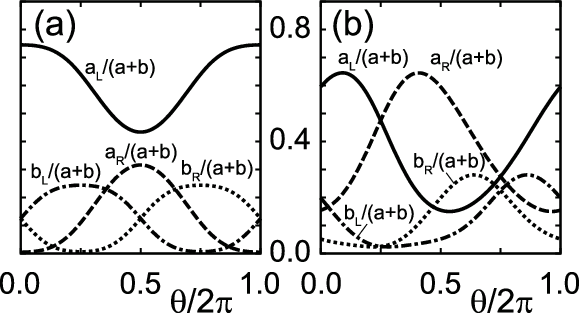
The present parametrization allows us to study each part of the current separately. In the first protocol, we use
| (60) | |||
| (61) | |||
| (62) |
The corresponding behavior of parameters , , , and is shown in Fig. 4(a). In this case, in the continuous-time case and the dominant contribution of the current comes from the dynamical part.


In the discrete-time case, we consider the process by using the discretized protocol. In Fig. 5, we plot the density of zeros at and . We find that each () in these cases takes a negative value. Then, the zeros continuously distribute on the negative real axis of with () where we set .
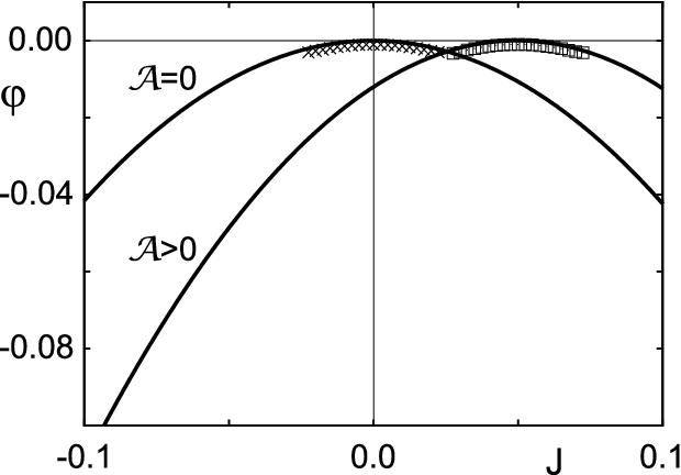
The corresponding rate function , calculated from Eq. (40), is shown in Fig. 6. We compare three results, exactly calculated from , from the approximation in Eq. (59), and from the simulations. As we see in Fig. 6, the result from zeros is consistent with that from the simulations. We also observe that the average current is well described by the approximation in Eq. (59).
We next consider the second protocol:
| (63) | |||
| (64) |
The corresponding behavior of parameters , , , and is shown in Fig. 4(b). In this case, the current in the continuous-time case is purely geometric. at each time, which means that the instantaneous dynamical current is exactly equal to zero. On the other hand, the flux in Eq. () is nonzero and we can observe a nonzero geometrical current.


We study how the geometric effect appears in the discrete-time case. At and , each () takes a negative value also in this case. The results of are shown in Fig. 7 and in Fig. 8.
In the case of , the current distribution is almost symmetric and the magnitude of the average current takes a small value. at small is well described by the approximation in Eq. (59). At , the protocol trajectory in parameter space does not enclose any surface and no geometric effect is observed. This result is significantly changed when we consider the case. The approximation in Eq. (59) does not give any reasonable result and we observe a nonzero average current. We find that simulation results are well fitted by the result from zeros. Since the condition of the adiabatic approximation is not obvious in the discrete-time case, it is remarkable to find that the geometric effect can be seen at small .
V Floquet–Magnus expansion
We have described the systems with small frequency by using the adiabatic approximation in the previous section. A similar systematic analysis is possible when takes a large value. When the transition-rate matrix drastically changes in short times, it is not appropriate to treat the discrete-time system and we consider the continuous-time case in this section.
In contrast to the adiabatic case, we can easily find two zeros in two-state systems and study the fluctuation effects on the current distributions. When the period of the modulation is very small, we can expect that the system is basically described by the averaged transition-rate matrix . The correction can be expressed by using a series expansion of the inverse frequency, which is known as the Floquet–Magnus expansion Magnus; BCOR.
We define the effective transition-rate matrix from the relation
| (65) |
where T denotes that the time-evolution operator is represented by the time-ordered product. In the Floquet–Magnus expansion, this effective matrix is represented as . is proportional to and the explicit forms at and 2 are given as follows:
| (66) |
| (67) | |||||
To give a concrete discussion, we treat the two-state case. Since the expansion keeps the trace of the transition-rate matrix invariant, we can generally write
where
| (71) |
and is defined in a similar way. The cumulant generating function is given by the largest eigenvalue of as
| (72) |
Up to the first order of the expansion, each element is given respectively by
| (73) | |||||
| (74) | |||||
| (75) | |||||
From these relations, we can find that the cumulant generating function takes a form
| (76) |
As in the zeroth order, the function is characterized by two zeros.
We can also examine the higher-order corrections. Although it is a difficult task to find the explicit forms, the expansion is systematically represented by multiple commutators. We find that up to the th order of the expansion
Then, the average current is given by
| (78) |
The current is generally characterized by many zeros and the number of the zeros increases as we increase the order of the expansion.


We show the result of the expansion up to the second order. We set the protocol in Eqs. (52)-(55) with
| (79) | |||
| (80) | |||
| (81) |
as shown in Fig. 9. The zeros are plotted in Fig. 10 and the corresponding current is in Fig. 11. We see that the current is properly described by using the zeros. At the zeroth order of the expansion, two zeros are located on the negative real axis. They change as functions of by taking into account the higher-order corrections. At the same time, when we increase the order of the expansion, different zeros appear around the origin and on the real axis far from the origin. These zeros are treated in pairs and give small corrections to the current as
| (82) |
at and .
To study the meaning of zeros, we examine how the fluctuation theorem is affected by the expansion. The rate is calculated from the Legendre transformation . In the expansion up to th order, the relation between and is obtained from
| (83) | |||||
with is uniquely determined for a given . Since it is difficult to obtain a compact form of the general solution, we discuss the cases where takes extremal values.
When the absolute value of is large, , the corresponding counting field is also large and we can evaluate
for and
for . Then, after some calculations we obtain
| (86) |
for . This relation implies that the affinity is given by the geometric mean of zeros. As we find in the above example, the product takes a finite value.
In the opposite limit at , the corresponding is obtained by solving
| (87) |
Then, is obtained as and
| (88) |
for .
VI Summary
We have studied dynamical Lee–Yang zeros in stochastic processes. As we mentioned in the Introduction, the distribution of zeros has complete information about the statistical properties of the processes. By discretizing the time variable, we can explicitly confirm that the number of zeros is related not to the number of states but to the number of events. We find nontrivial distributions of zeros even in simple two-state processes. The distribution of zeros is related to the current distributions and we expect that our discrete-time result can be confirmed experimentally by measuring processes with rare events.
Since our analysis is restricted to simple two-state systems, the zeros distribute only on the negative real axis of . In statistical mechanics, thermal phase transitions can be found by studying the distribution of zeros. The locations of zeros represent the boundary of different phases in complex plane. We have not found closed boundaries in the present analysis. It may be an interesting problem to study more complex systems such as quantum dot systems coupled with external reservoirs treated in previous studies UEUA; SMY17.
One of the important findings in the present study is that the method can be applied in the case of the periodically oscillating transition rate. In the adiabatic case with slowly varying transition-rate matrix, the property of the density of zeros is dependent on the geometric properties of the protocols. We also find in the fast-driving regime of the continuous-time case that the number of zeros depends on the order of the expansion. These results show that it is important to study global distributions of zeros to characterize the dynamically fluctuating systems instead of using a few number of zeros. The distribution also reflects a fundamental symmetry of the system. We expect that the principle of nonequilibrium thermodynamics can be studied along with the method developed in the present study.
Acknowledgments
We thank Y. Utsumi for valuable comments. K.T. was supported by JSPS KAKENHI Grants No. JP20K03781 and No. JP20H01827.
References
References
- (1) D. J. Evans, E. G. D. Cohen, and G. P. Morriss, Probability of Second Law Violations in Shearing Steady States, Phys. Rev. Lett. 71, 2401 (1993).
- (2) G. Gallavotti and E. G. D. Cohen, Dynamical Ensembles in Nonequilibrium Statistical Mechanics, Phys. Rev. Lett. 74, 2694 (1995).
- (3) G. E. Crooks, Entropy production fluctuation theorem and the nonequilibrium work relation for free energy differences, Phys. Rev. E 60, 2721 (1999).
- (4) L. S. Levitov and G. B. Lesovik, Charge distribution in quantum shot noise, JETP Lett. 58, 230 (1993).
- (5) L. S. Levitov, H.W. Lee, and G. B. Lesovik, Electron counting statistics and coherent states of electric current, J. Math. Phys. 37, 4845 (1996).
- (6) D. A. Bagrets and Y. V. Nazarov, Full counting statistics of charge transfer in Coulomb blockade systems, Phys. Rev. B 67, 085316 (2003).
- (7) K. Saito and Y. Utsumi, Symmetry in full counting statistics, fluctuation theorem, and relations among nonlinear transport coefficients in the presence of a magnetic field, Phys. Rev. B 78, 115429 (2008).
- (8) C. N. Yang and T. D. Lee, Statistical theory of equations of state and phase transitions. I. Theory of condensation, Phys. Rev. 87, 404 (1952).
- (9) T. D. Lee and C. N. Yang, Statistical theory of equations of state and phase transitions. II. Lattice gas and Ising model, Phys. Rev. 87, 410 (1952).
- (10) M. E. Fisher, The Nature of Critical Points, Lectures in Theoretical Physics Vol. VII C (University of Colorado Press, Boulder, 1965).
- (11) A. G. Abanov and D. A. Ivanov, Allowed Charge Transfers between Coherent Conductors Driven by a Time-Dependent Scatterer, Phys. Rev. Lett. 100, 086602 (2008).
- (12) D. A. Ivanov and A. G. Abanov, Phase transitions in full counting statistics for periodic pumping, Europhys. Lett. 92, 37008 (2010).
- (13) C. Flindt and J. P. Garrahan, Trajectory Phase Transitions, Lee–Yang Zeros, and High-Order Cumulants in Full Counting Statistics, Phys. Rev. Lett. 110, 050601 (2013).
- (14) Y. Utsumi, O. Entin-Wohlman, A. Ueda, and A. Aharony, Full-counting statistics for molecular junctions: Fluctuation theorem and singularities, Phys. Rev. B 87, 115407 (2013).
- (15) J. M. Hickey, C. Flindt, and J. P. Garrahan, Intermittency and dynamical Lee–Yang zeros of open quantum systems, Phys. Rev. E 90, 062128 (2014).
- (16) R. S. Souto, A. Martín-Rodero, and A. L. Yeyati, Analysis of universality in transient dynamics of coherent electronic transport, Fortschr. Phys. 65, 1600062 (2016).
- (17) K. Brandner, V. F. Maisi, J. P. Pekola, J. P. Garrahan, and C. Flindt, Experimental Determination of Dynamical Lee–Yang Zeros, Phys. Rev. Lett. 118, 180601 (2017).
- (18) R. S. Souto, A. Martín-Rodero, and A. L. Yeyati, Quench dynamics in superconducting nanojunctions: Metastability and dynamical Yang–Lee zeros, Phys. Rev. B 96, 165444 (2017).
- (19) B.-B. Wei and R.-B. Liu, Lee–Yang Zeros and Critical Times in Decoherence of a Probe Spin Coupled to a Bath, Phys. Rev. Lett. 109, 185701 (2012).
- (20) X. Peng, H. Zhou, B.-B. Wei, J. Cui, J. Du, and R.-B. Liu, Experimental Observation of Lee–Yang Zeros, Phys. Rev. Lett. 114, 010601 (2015).
- (21) D. J. Thouless, Quantization of particle transport, Phys. Rev. B 27, 6083 (1983).
- (22) N. A. Sinitsyn and I. Nemenman, The Berry phase and the pump flux in stochastic chemical kinetics, Europhys. Lett. 77, 58001 (2007).
- (23) W. Magnus, On the exponential solution of differential equations for a linear operator, Commun. Pure Appl. Math. 7, 649 (1954).
- (24) S. Blanes, F. Casas, J. Oteo, and J. Ros, The Magnus expansion and some of its applications, Phys. Rep. 470, 151 (2009).
- (25) K. Takahashi, K. Fujii, Y. Hino, and H. Hayakawa, Nonadiabatic Control of Geometric Pumping, Phys. Rev. Lett. 124, 150602 (2020).
- (26) K. Takahashi, Y. Hino, K. Fujii, and H. Hayakawa, Full counting statistics and fluctuation-dissipation relation for periodically driven two-state systems, J. Stat. Phys. 181, 2206 (2020).
- (27) M. V. Berry, Quantal phase factors accompanying adiabatic changes, Proc. R. Soc. London, Ser. A 392, 45 (1984).