A New Modeling of Classical Folds in Computational
OrigamiThanks: Supported by JSPS KAKENHI Grant No.16K00008
Affiliation: University of Tsukuba
Tsukuba 305-8573, Japan
Abstract
This paper shows a cut along a crease on an origami sheet makes simple modeling of popular traditional basic folds such as a squash fold in computational origami. The cut operation can be applied to other classical folds and significantly simplify their modeling and subsequent implementation in the context of computational origami.
1 Introduction
Origami attracts the minds of people all over the world. Some are interested in its geometric aspects, and others in artistic or recreational elements, so-called traditional origami. Although both origami categories rely on a single notion of paper folding, their methodologies differ significantly due to the pursuits’ objectives and goals. In this paper, we focus on traditional origami.
We can find numerous origami artworks in web pages, books and technical papers; some are in the realm of artistic creation, and others are pieces of origami works for recreation and educational purposes. The origami creators’ interest lies more in artistic creativity than general folding rules in the first category. In contrast, in the second category, the underlying motivation is to find a finite number of basic fold rules. Although in 2D (two dimensional) origami geometry, we can obtain such a collection of rules, in traditional origami, we are more liberal to collect fold rules since the set may be open. Nevertheless, we give some basic fold rules that we use in traditional origami. We start from the description of the web pages [4].
We understand the 2D origami geometry to the extent that we do the 2D Euclidean geometry in terms of the constructible points in the two geometries. Namely, the set of the points constructible by Huzita-Justin’s fold rules [6, 10] is the strict superset of intersecting points of the circles and the lines made by a straightedge and a compass - the construction tool of Euclidean geometry. Alperin gave a more concise description of this fact in the language of fields [2].
However, we do not have a clear view of formalization of traditional origami. The formalization of traditional origami, in its entirety, is not our intended goal. Instead, we prefer to model some of the crucial and sophisticated operations using the results of the accumulated formalization efforts (e.g., [11, 5, 4]).
In our earlier work, we presented an abstract origami system [8]. It involves the notions of two relations on the set of origami faces. By them, we can model the superpositions of pieces of origami faces. The superpositions of the faces make origami look like a three-dimensional (3D) object. To superpose faces intriguingly makes the origami artistic or a thing that many people fancy to construct. Classical folds have been discovered and elaborated over time to the present day to cater to these desires. For example, on the web pages of corsoyard.com, they show more than ten classical folding techniques [4]. As typified by the squash fold and inside-reverse fold, the classical fold intricately combines several simple folds. One squash fold, for example, requires the simultaneous three simple folds, i.e., mountain or valley fold, subjected to non-trivial constraints. The combination of those three folds will not afford us simple modeling of the fold.
This paper shows a cut along a crease makes simple modeling of a squash fold in computational origami. The cut operation can be applied to other classical folds and significantly simplify their modeling and subsequent implementation in the context of computational origami.
2 Preliminary
Let be a finite set of (origami) faces, be a binary relation on , called adjacency relation and be a binary relation on , called superposition relation. An abstract origami is a structure . We abbreviate abstract origami to AO. We denote the set of AOs by . An abstract origami system is an abstract rewriting system [3] , where is a rewrite relation on , called abstract fold.
For , we write when is abstractly folded to . We start an origami construction with an initial AO and perform an abstract fold repeatedly until we obtain the desired AO. Usually, we start an origami construction with a square sheet of paper. This initial sheet of paper is abstracted as a structure having a single distinguished face denoted by the numeral . Then, the initial AO is represented by . We could use any symbol to denote the initial face. Still, we find it convenient to use the numeral ’’ as we can interpret it as a numeric value to generate the denotation of the new faces during the construction. We will see in the concrete examples that when we fold face , the face is divided into two faces and . We use this convention in this paper and the realization of the data structure of the computational origami system Eos [9]. Suppose that we are at the beginning of step of the construction, having AO . We perform an abstract fold and obtain a next AO . Thus, we have the following -sequence.
An abstract origami construction is a finite -sequence of AOs.
In concrete terms, the operation can be a Huzita-Justin’s fold rule, a mountain fold, a valley fold, etc., each requiring different kinds of arguments. For further details, refer to [7], Chapter 7.


3 A motivating example
We consider a squash fold since it is used frequently in traditional origami. See, for example, a popular book on origami [12].
Figure 1 shows an origami house that most children can compose when they learn the recipe of the origami house. The only non-trivial steps are the squash folds on the right- and left-hand roofs of the house. Figures 2 and 3 show the selected AOs in the construction sequence. When we show AOs in the figures, we show their geometrical interpretation rather than express them symbolically.


We briefly explain how we obtain each AO in the sequence.
-
Step 1: We start with the initial origami , which we represent geometrically in 2(a).
-
Step 2: Fold to bring D to A in Fig. 2(b).
-
Steps 3 and 4: Fold to bring D to C, and then unfold in Fig. 2(c).
-
Steps 5 and 6: Fold to bring F to C, and then unfold in Fig. 2(d).
-
Step 7: Fold to bring C to H in Fig. 2(e).
-
Steps 8 and 9: Fold to bring F to R, and then unfold in Fig. 3(a).
From the construction sequence, we see a slit below faces JSF and SJR, i.e., square JRSF in Fig. 3(a). We pull point J slightly upward and make a small space below JRSF. Then, we move segments SF and SJ with S fixed, such that SF overlays SR. By this movement, we squash face JSF onto the area to the right of segment SR. After the squash, the rotated segment SF and non-moved segment SR, as a whole, look like a ridge and a valley that departs at S. This fold invokes three simultaneous face moves by three fold lines. It is a sophisticated motion, and none of Huzita-Justin rules can cope with it. In applying Huzita-Justin rules, we can employ only one fold line in a single fold. If we allow a cut along crease SJ, we simplify the moves of the involved faces. After we complete this squash operation, we glue the edges separated by the cut operation. The algorithm of squash fold with a cut in the next section makes clear the involved face moves.
To complete the construction of the origami house, we perform the same sequence of fold operation on the left part of the rectangle DBFE, although in a mirror fashion across line IC.
4 Squash fold with a cut
In its simplest form, we perform a squash fold on a four-layered square shown in Fig. 4(e).


We can visualize more clearly by expanding the vertical gap between the faces, as in Fig. 5.

We have . We could represent the relations and by the usual notation of a set of pairs of the denotations of the faces in , but to facilitate the analysis of the relations, we use the graphs of and . Figures 6(a) and 6(b) show the relations and , respectively. We note that faces and are adjacent. We can also observe the adjacency of faces and in Figs. 4(e) and 5. The dotted line borders faces and . As a convention, a dotted line denotes a valley crease in our graphics visualization.


To reason about the geometric properties of 3D origami, we extensively use tools of graph theory and 3D visualizations. We needed to develop tools of the latter by ourselves as part of Eos.
With this preparation, we now describe the algorithm of a squash fold with a cut.
Algorithm Squash fold with a cut
- 1.
- 2.
Fold face 10 along ray IG (cf. Fig. 7(a)).
- 3.
Fold face 11 along ray FI (cf. Fig. 7(b)).
- 4.
Fold to bring point F to point G. Equivalently, fold along segment IC (cf. Fig. 7(c)).
- 5.
Glue the edge separated at Step 1, i.e., edge IB.
We show the result of the execution of the algorithm in 3D, together with the associated adjacency and superposition graphs in Fig.9.


The curved surfaces between the edges
of the two overlapping faces show that they are connected.


Once we design the algorithm of the squash fold, we can easily abstract the algorithm into a function called SquashFold. Then, we treat the call of SquashFold with appropriate arguments as if the squash fold were a single operation. We describe SquashFold in the syntax of Wolfram Language of Mathematica [13]. Function SquashFold is incorporated into Eos. SquashFold0 below performs the algorithm.11
1
We omit optional arguments in function definitions for brevity. It is one of the rewrite rules that define function SquashFold. We have other rules for different kinds of arguments of the squash fold.
SquashFold0[{below_,above_},{bottom:Ray[P_,Q_],
 ridge:Ray[R_,P_]}]:=
(CutEdge[{below,above}];
 ValleyFold[below,bottom];ValleyFold[above,ridge];HO[R,Q];
 GlueEdges[$cutEdge])
The first line and the second (to the left of :=) line of the program is a left-hand side of a rewrite rule in which we specify input arguments; below and above are faces that will become below and above the faces of the squashed part of the origami. In this case, the variables below and above are bound to 10 and 11, respectively, when we execute the following function call.
SquashuFold0[{10,11},{Ray["I","G"],Ray["F","I"]}]
The other variables, i.e., variables P, Q, and R, are bound to "I", "G", and "F", respectively. Note that we enclose point names with double quotation marks when we write Eos programs.
The third to fifth lines of the program are a constituent of the right-hand side of the rewrite rule, and their meanings are self-explanatory, except for the global variable $cutEdge, which holds the encoding of the cut edges. The fourth line is the program’s nucleus. It performs lines 2, 3, and 4 of Algorithm Squash fold with a cut. In the program, we evaluate the functions with specific names to its operations, i.e., functions corresponding to valley fold, valley fold and Huzita-Justin rule O2.
In summary, we have observed that at the level of abstract origami rewriting.
We call the composition of rewrites a rewrite of a squash fold.
We can also observe that the adjacency graphs of and are the same.
5 Basic folds in traditional origami
We remarked in the introduction that origamists are more interested in the final origami shapes than the rule set of folds in traditional origami practice. Nevertheless, it is convenient to have a small collection of basic folding rules. In this section, we present some candidates of such basic rules.
- •
Huzita-Justin rules (seven rules, O1 – O7,)
- •
Mountain fold and valley fold
- •
Inside-reverse fold
- •
Outside-reverse fold
- •
Rabbit-ear fold
- •
Pleat fold and crimp-pleat fold
5.1 Huzita-Justin rules
Huzita and Justin proposed the rules in the context of 2D origami geometry. They are the alternatives to a compass and a straightedge of the 2D Euclidean geometry. The rules define a fold line, and we fold the origami along it. We use the fold line to perform either a mountain fold or a valley fold. We restrict the use of Huzita-Justin rules to geometric origami, primarily. However, we have seen with Huzita-Justin rules we can construct a variety of origami works.
5.2 Mountain fold and valley fold
Mountain and valley folds are applicable, in Eos, to a set of the faces of the abstract origami. They can be multi-layered. Eos automatically computes the target faces on which it performs folds. Thus, Functions MountainFold and ValleyFold can take arguments of a list of origami faces and a fold line. We can perceive the difference between “mountain” and “valley” when we unfold the origami immediately after the fold. If we see the crease made by the fold line that looks like a valley, it is a valley fold; if the crease looks like a mountain ridge, it is a mountain fold.
These are the most basic fold operations. We note that fold lines have no association with directions. Therefore, we use a ray instead of a line when Eos cannot determine the direction of the face movement in folding by other parameters. With the use of rays, we can observe the right-/left-hand side of the line. We adopt the right-handed system and move the faces to the right of the ray when we fold the origami along the ray(line).
In the program of SquashFold0, we already used two valley folds and one Huzita-Justin rule O2. We may replace the rule O2 with a fold along a ray that forms the perpendicular bisector of Segment[R, Q]. However, the O2 rule is applicable in this case since the target faces together form a flat plane. Furthermore, it is easier to reason about the geometric properties with Huzita-Justin rules.
5.3 Inside reverse fold and outside reverse fold
An inside reverse fold and an outside reverse fold are very similar operations. Suppose we have a pair of overlapping faces that share an edge. We fold the two faces by moving the part of the faces as in Fig. 10 and Fig. 11. The figures clearly show what actions are involved. We need two (but the same) rays to perform mountain and valley folds simultaneously. The inside reverse and the outside reverse folds require two folds in a restricted way. Hence, we see that we cannot apply Huzita-Justin rules. We can use the cut as in the squash fold. We show programs of the inside reverse fold and the outside reverse fold, too. They are easy to understand since we use the same set of functions similarly.
We obtain the origami shape in Fig. 10 by executing:
InsideReverseFold[{5,7},Ray["F","E"]]
where function InsideReverseFold is defined by
InsideReverseFold[{below_,above_},ray_] :=
 (CutEdge[{below,above}];
  MountainFold[above,ray,InsertFace->below];
  ValleyFold[below,ray,InsertFace->above];
  GlueEdges[$cutEdge])
The numerals 5 and 7 of the faces are obtained by the visualization tools, which are not discussed here.


Likewise, we obtain the origami in Fig. 11 by executing:
InsideReverseFold[{5,7},Ray["F","E"]]
where function OutsideReverseFold is defined by
OutsideReverseFold[{below_,above_},ray_] :=
 (CutEdge[{below,above}];
  ValleyFold[above,ray];
  MountainFold[below,ray];
  GlueEdges[$cutEdge])


5.4 Rabbit ear fold
We show in Figs. 12(a) - (f) selected (geometric representation of) AOs in the construction sequence of a rabbit ear fold. We can see an erected tab on the plane in Fig. 12(f). We apply Function RabbitEarFold to with the following arguments (inside RabbitEarFold[...]).
RabbitEarFold[{11,9},{Ray["F","A"],Ray["F","H"],
  Ray["F","D"]}]
To be precise, the function RabbitEarFold takes a pair of faces and three rays. It makes a tab that looks like a rabbit ear standing on the isosceles triangular plane (cf. Fig. 12(e)). The three rays start from the same point , and we represent the three rays as Ray[, ], Ray[, ], and Ray[, ]. is a right-angle triangle whose hypotenuse is , and is another right-angle triangle whose hypotenuse is . The function constructs rabbit ear .
RabbitEarFold[{below_,above_},
 {ridge_,base_,hypotenuse_}] :=
  (CutEdge[{below,above}];
   ValleyFold[below,Rev[ridge]];
   ValleyFold[base];
   ValleyFold[Rev[hypotenuse]];
   ValleyFold[ridge];
   GlueEdges[$cutEdge])
In the above, we have Rev[Ray[,]]Ray[, ] for any points and .
During the rabbit ear fold, we cut the edge FE of . Then, we perform four valley folds with supplied arguments. To make the intended faces move, we need to define carefully the ray along which we perform the fold. The fold of to is a valley fold along Ray[H, F] by . The value is an additional argument of VallyFold, and it specifies the angle of rotation during the valley fold. It makes the ”ear” part stand upright as shown in Fig. 12(e).


5.5 Pleat fold and pleat crimp fold
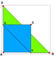
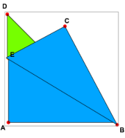
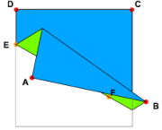
A pleat is a shape pattern made of cloth or flexible flat material folded along two fold lines. In origami, a fold that makes a pleat, such as shown in Fig. 13, is called a pleat fold. In the figure, we only show three examples of pleat folds. The line segments DB and EF are not necessarily in parallel. We often use two lines sharing a point. In the pleat crimp fold, we shortly explain, we use the configuration that two line segments meet at one end.
A pleat fold is easy to perform. A pleat fold becomes more complex and exciting when combined with folds similar to an outside (or inside) reverse fold. In Fig. 14, we show an origami construction that makes up a pleat crimp. The idea of realizing a pleat crimp is to divide the origami into two and apply a pleat fold to each piece. After the pleat folds on each piece, we glue them together. We have two ways of making a crimp. The one shown in Fig. 14 has a pleat outside. Figure 15 shows the other case that the pleats are inside.


6 Concluding remarks
We have shown that a cut along a crease enables modeling the classical fold ”squash fold” more abstract and simplifies the implementation in computational origami. Using a cut operation, we can reduce the squash fold to a sequence of valley folds and a Huzita-Justin rule. We explained the model as an abstract origami rewrite system. Graph representation of abstract origami reveals properties among origami faces which, otherwise, would be invisible by usual origami by hand. We have also shown that we can model other popular traditional folds by cut and glue crease edges.
References
- [1]
- [2] Roger C. Alperin (2000): A Mathematical Theory of Origami Constructions and Numbers. New York Journal of Mathematics 6, pp. 119–133.
- [3] Marc Bezem & Jan Willem Klop (2003): Abstract reduction systems, chapter 1, pp. 7 – 23. Term Rewriting Systems, Cambridge University Press.
- [4] corsoyard.com: Origami Basic Technics. Available at http://corsoyard.com/origami/origami-basic/#basic5.
- [5] Folds.net (2005): Origami Diagrams on the Web. Available at http://www.folds.net/tutorial/index.html.
- [6] Humiaki Huzita (1989): Axiomatic Development of Origami Geometry. In Humiaki Huzita, editor: Proceedings of the First International Meeting of Origami Science and Technology, Ferrara, Italy, pp. 143 – 158.
- [7] Tetsuo Ida (2020): An introduction to Computational Origami. Texts and Monographs in Symbolic Computation, Springer Internatonal, 10.1007/978-3-319-59189-6.
- [8] Tetsuo Ida & Hidekazu Takahashi (2010): Origami fold as algebraic graph rewriting. J. Symb. Comput. 45(4), pp. 393–413, 10.1016/j.jsc.2009.10.002.
- [9] Tetsuo Ida, Dorin Tepeneu, Bruno Buchberger & Judit Robu (2004): Proving and Constraint Solving in Computational Origami. In: Proceedings of the 7th International Symposium on Artificial Intelligence and Symbolic Computation (AISC 2004), Lecture Notes in Artificial Intelligence 3249, pp. 132–142, 10.1007/978-3-540-30210-0_12.
- [10] Jacques Justin (1986): Résolution par le pliage de l’équation du 3e degré et applications géométriques. L’Ouvert (42), pp. 9 – 19.
- [11] Robert J. Lang (2003): Origami Design Secrets: mathematical methods for an ancient art. ISBN-10 : 1568811942, A K Peters/CRC Press, 10.1201/b10706.
- [12] Shufunotomosha, editor (2011): Popular Origami Best 50 (in Japanese). Shufunotomosha. English guidance by M. Aoki is provided.
- [13] Wolfram Research, Inc. (2012): Mathematica 12.3.