Resolvent-based tools for optimal estimation and control via the Wiener-Hopf formalism
Abstract
The application of control tools to complex flows frequently requires approximations, such as reduced-order models and/or simplified forcing assumptions, where these may be considered low-rank or defined in terms of simplified statistics (e.g. white noise). In this work, we propose a resolvent-based control methodology with causality imposed via a Wiener-Hopf formalism. Linear optimal causal estimation and control laws are obtained directly from full-rank, globally stable systems with arbitrary disturbance statistics, circumventing many drawbacks of alternative methods. We use efficient, matrix-free methods to construct the matrix Wiener-Hopf problem, and we implement a tailored method to solve the problem numerically. The approach naturally handles forcing terms with space-time colour; it allows inexpensive parametric investigation of sensor/actuator placement in scenarios where disturbances/targets are low rank; it is directly applicable to complex flows disturbed by high-rank forcing; it has lower cost in comparison to standard methods; it can be used in scenarios where an adjoint solver is not available; or it can be based exclusively on experimental data. The method is particularly well-suited for the control of amplifier flows, for which optimal control approaches are typically robust. Validation of the approach is performed using the linearized Ginzburg-Landau equation. Flow over a backward-facing step perturbed by high-rank forcing is then considered. Sensor and actuator placement are investigated for this case, and we show that while the flow response downstream of the step is dominated by the Kelvin-Helmholtz mechanism, it has a complex, high-rank receptivity to incoming upstream perturbations, requiring multiple sensors for control.
1 Introduction
Flow control is a challenging problem both from the academic perspective and in terms of concrete applications, where problems such as laminar-to-turbulent transition, drag reduction, and flow-induced vibration are of practical concern [1, 2, 3, 4, 5, 6]. The difficulties arise from the non-linearity of flow dynamics, which is often avoided by considering a linearized system. Nevertheless, it is not clear how to model the neglected non-linear terms, and effective methods to determine the optimal location of sensors and actuators are still a topic of research. Among the linear control strategies presently available, inverse feed-forward, wave-cancellation, optimal and robust control are popular choices. Throughout this work, by optimal and robust control we mean the corresponding linear control approaches.
In flows dominated by convection, wave-cancellation has been proposed as a simple-but-effective control strategy. Waves are identified by upstream sensors, and actuators situated between the sensors and targets act to minimize perturbations at the target location [7]. Although the approach is not guaranteed to be causal, in so far as computation of the actuation signal may require future sensor readings, causality can be imposed by ignoring the non-causal part of the control kernel. This has been shown to closely reproduce optimal control when there is sufficient distance between sensors, actuators, and targets [8]. While this can significantly reduce the effectiveness of the controller [9], the approach has been successfully used in numerous studies [10, 11, 12]. A similar approach was used by [5], where opposition control based on the resolvent operator was performed. Adaptive control strategies are often similar to wave-cancellation approaches, but use additional downstream sensors to adapt the control law to changes in the flow [13, 14].
Optimal control, on the other hand, minimizes a quadratic cost functional [15], frequently associated with the mean perturbation energy. This approach provides a maximal reduction of perturbation energy and has been used to control flow instabilities [16] or to reduce the receptivity of a flow to disturbances [17, 18, 19, 20, 21, 22], to delay transition to turbulence, for instance.
However, the robustness of optimal control may be hindered by feedback between actuators and sensors and/or by small errors in the flow model. In some cases, such issues may even cause the control law to further destabilize the system. While the model can be accurately known in some scenarios, for instance when simulating transitional flows subject to small disturbances, applications in off-design conditions, or in cases where non-linear dynamics are important, will generally result in a reduction of the accuracy with which the linear model represents the physical system. Robust control allows a balance to be struck between the cost-functional reductions and the control robustness: at the cost of achieving lower energy reduction than optimal control, robust control can tolerate higher modeling errors. This kind of approach has been used in several recent studies [23, 24, 6]. Robust control is particularly important for the control of oscillator systems where actuators are frequently situated upstream of sensors [15]. For this kind of configuration, optimal control is typically not robust [25].
There are, however, many scenarios where optimal control is robust. [25] showed that this is the case for amplifier flows, where sensors are typically located upstream of actuators. [18] arrived at a similar conclusion for the control of boundary layer disturbances, where the optimal control was found to be robust to changes in Reynolds numbers and pressure gradients. Our study is focused on this scenario: the development of optimal control for amplifier flows.
The usual approach to obtain optimal control laws involves solution of Riccati equations. The computational cost grows rapidly with the number of degrees of freedom (DOFs) of the system. As problems in fluid mechanics typically have many DOFs, methods based on the solution of Riccati equations are impractical. A standard way of dealing with this issue is to base control design on a reduced-order models (ROMs) [15]. Several bases have been used to obtain ROMs, such as proper orthogonal decomposition (POD) modes [26], eigenmodes [27], and balanced modes [15, 17]. The eigen-system realization (ERA) algorithm [28] was shown to be equivalent to a ROM based on balanced modes, with only a fraction of the costs when external disturbances are low-rank [29]. A drawback of such techniques is that control laws obtained from these ROMs are not guaranteed to be optimal when applied to the full system. Model reduction with balanced modes has upper-error bounds for modelling open-loop systems, but even when the open-loop system is accurately represented by the ROM, a control law based on the ROM can be ineffective when applied to the original problem [30, page 349].
Several approaches exist for obtaining estimation and control laws for the full system. Optimal estimation and control gains for the full system can be obtained iteratively [31, 32]. This, however, requires integration of a large auxiliary system for real-time application; this adds significant cost when used in a numerical simulation and is likely unfeasible for experimental implementation. Alternatively, the control law can be reduced a posteriori (design-then-reduce), instead of being designed based on a ROM (reduce-then-design). Another approach applicable to the full system is to use estimation strategies using an ensemble Kalman filter [33]. However, this requires the integration of multiple realizations of the full system, which adds significant computational cost when applied to numerical solutions.
Control strategies are highly dependent on actuator and sensor placement, and the optimal choice is often unclear. As ROMs are frequently derived for a specific set of sensors and actuators, studies of the role of their placement for control often rely on the derivation of multiple ROMs. An example is the study of [34], in which an ERA ROM was required for each sensor position. This highlights the role of reduced-order models in studies of sensor and actuator placement and how this can be costly. As sensor and actuator positioning substantially impacts the control strategy [35, 36, 34, 37], it is of interest to be able to obtain control laws without having to rely on ROMs for each possible choice of sensor and actuator.
Most approaches used for flow control typically require simplified forcing assumptions, frequently modelled as white-in-time noise. Although complex spatial-temporal forcing colour can be used in the Kalman-filter framework, the approach requires use of an expanded system that filters a white noise input to create a coloured noise, with the extra assumption that the forcing CSD is a rational function of the frequency [38]. Simplified forcing-colour models are thus typically used to avoid this complexity. However, it has been shown that the use of realistic spatiotemporal forcing colour is crucial for accurate estimation of complex flows [39, 40, 41]. This is an indication that control can be considerably enhanced if realistic forcing models are used.
Another approach to estimation and control is possible using the Wiener-Hopf formalism. An optimal non-causal estimation method, known as a Wiener filter [42, 43], and optimal control strategies, known as Wiener regulators [44, 45, 46], can be obtained based on cross-spectral densities (CSDs) between sensors, actuators, and flow states. Although well described in the control literature, their potential for flow control has not been appropriately explored. To the best of the authors’ knowledge, [47] is the only work in which the formalism has been used for flow control. Difficulties in solving the associated Wiener-Hopf problems limited that study to the use of one sensor and one actuator, and the significant cost of converging the CSDs probably hindered further application of the method.
Wiener-Hopf problems appear when causality constraints are imposed on the estimation and control kernels. The Wiener-Hopf method has been used in the fluid mechanics community to obtain solutions to linear problems with spatial discontinuities, such as acoustic scattering by edges [48, 49]. Solutions to this class of problem are typically based on a factorization of the Wiener-Hopf kernel into components that are regular on the upper/lower halves of the complex frequency plane. Such factorization can be achieved analytically only for scalar problems [50, 49] and for some special classes of matrices [51, 52]. Lacking general analytical solutions, several numerical approaches can be used [53, 54, 55, 56]. The potential of the method for estimation and control comes from the fact that the size of the matrices to be factorized scales with the number of sensors and actuators, in contrast to control strategies based on solutions of algebraic Riccati equations that scale with the system’s size.
While the use of a linear control strategy for non-linear systems has clear limitations, i.e., it is expected to work only when the disturbances around a reference flow can be reasonably approximated by a linear model, there are many examples in the literature (several of which were cited above) that show how the approach is useful in a broad variety of flows.
The objective of our study is to obtain a method for real-time estimation and control that avoids some of the drawbacks of previous approaches. To achieve this, we strategically combine three pre-existing tools: the Wiener-Hopf regulator for flow control [47]; a numerical method to solve matrix Wiener-Hopf problems [54]; and matrix-free methods for obtaining the resolvent operator of large systems [40, 57, 58]. Combining these tools provides a novel method that can, for the first time, simultaneously handle complex forcing colour and be applied directly to large systems without the need for a priori model reduction, allowing parametric investigation of sensor/actuator placement at low cost when forcing/targets are low rank. To the best of the authors’ knowledge, this is also the first time that the Wiener-Hopf regulator is constructed from first principles, i.e., from the linearized equations of motion and a model of the forcing, as in the LQG framework. This construction provides physical insights on the structures that can be estimated and controlled. The approach can also be used to improve wave-canceling strategies [59, 8, 13, 12, 9], minimizing the effect of kernel truncation.
The method can be viewed as an extension of the resolvent-based estimation methods recently developed by [60] and [40]. In the former study, a resolvent-based approach was developed to estimate space-time flow statistics from limited measurements. The central idea is to use the measurements to approximate the non-linear terms that act as a forcing of the linearized Navier-Stokes equations, which in turn provide an estimate of the flow state upon application of the resolvent operator in the frequency domain. The latter study extends this resolvent-based methodology to obtain optimal estimates of the time-varying flow state and forcing. The estimator is derived in terms of transfer functions between the measurements and the forcing terms and can be written in terms of the resolvent operator and the CSD of the forcing. However, these methods are nominally non-causal, making them appropriate for flow reconstruction but limiting their applicability for flow control.
The method developed in the current paper follows that of [40], but with additional constraints to enforce causality. It is these constraints that lead to the aforementioned Wiener-Hopf problem. The causality of the new resolvent-based estimator makes it applicable for real-time estimation, and we use a similar approach to develop an optimal resolvent-based controller. The resulting estimation and control methods are thus obtained directly for the full-rank flow system, without requiring ROMs, and they make use of the spatiotemporal forcing statistics, thus avoiding the simplified forcing assumptions that can lead to significant reductions in performance.
The paper is structured as follows. The derivation of optimal estimation and control kernels based on the Wiener-Hopf formalism are constructed in § 2, and solutions are compared to those obtained from algebraic Riccati equation using a linearized Ginzburg-Landau problem. Implementation of the method using numerical integration of the linearized system and using experimental data are described in § 3. An application to flow over a backward-facing step is presented in § 4. Final conclusions are drawn in § 5. An introduction to Wiener-Hopf problems (which appear in § 2) and their solution is presented in Appendix A.
2 Estimation and control using Wiener-Hopf methods
In what follows, we define the linear system considered, followed by the derivation of optimal estimation and control kernels based on the Wiener-Hopf approach. Optimality here is defined in terms of quadratic cost functionals. An approach to recover estimation and control gains from the proposed approach is presented. The derivation for full-state control is presented in Appendix B.
2.1 System definition
We consider the linear time-invariant system
| (1) |
where represents the flow state, is an unknown stochastic forcing, which can represent external disturbances and/or non-linear interactions [61], represents flow actuation used for control, is a set of system observables, is measurement noise, and is a set of targets for the control problem, for instance, perturbations at a given position or surface loads, to be minimized. The system evolution is described by the matrix , representing the linearized Navier-Stokes operator. The matrices , , , and determine the spatial support of external disturbances, actuators, sensors, and targets, as in [62]. Forcing and sensor noise are modelled as stochastic zero-mean processes with two-point space-time correlations given by
| (2) | ||||
| (3) |
with representing the adjoint operator using a suitable inner product and representing the ensemble average. We emphasize that these forcing and noise statistics are more general than those assumed in the derivation of the Kalman filter and LQG control, in which they must be uncorrelated in time. A frequency-domain representation of the two-point correlation is given by the CSDs
| (4) | ||||
| (5) |
Note that this differs from the standard definition, i.e., , with representing the conjugate transpose of the matrices; this modified definition simplifies the derivations that follow.
Throughout this work, we assume the system to be stable, i.e., all eigenvalues of A, i.e., for which has non trivial solutions, lie in the lower-half plane. As discussed in § 1, optimal control strategies are best suited for amplifier flows, which satisfy this stability requirement.
It is useful to split (1) into two systems, one of which is driven by the forcing and includes sensor noise,
| (6) |
and another noiseless system driven by actuation only,
| (7) |
The original system can be recovered adding the variables with subscripts “1” and “2”, that is,
| (8) |
The derivations that follow make use of the frequency-domain form of these equations. Taking a Fourier transform of (6) and (7) yields the input-output relationships
| with | (9) | |||||
| with | (10) | |||||
| with | (11) | |||||
| with | (12) |
where
| (13) |
is the resolvent operator. Note that the above input-output relations are exact within the linearized model used here, and thus has the same limitation as any linear modelling of the original non-linear system, i.e., treating the non-linear interactions as exogenous stochastic noise. This framework is shared by all linear control laws that have been developed.
2.2 The estimation problem
Before deriving the optimal causal estimator that we seek, we first briefly review the derivation of the optimal non-causal estimator [40]. We will see later that the two cases are closely related but that imposing causality leads to the appearance of an additional term. We focus on the uncontrolled estimation problem, i.e. , thus making (1) and (6) equivalent.
The optimal estimator minimizes the cost functional
| (14) |
defined in terms of the estimation error
| (15) |
where is the target, i.e., the quantity to be estimated, and is its estimate. Note that full-state estimation is recovered using .
We seek an estimate of the targets in the form of a linear combination of sensor readings, in the form of
| (16) |
where the subscript is a reminder that the kernel, , is, in general, non-causal, and is its Fourier transform. Expanding (14) leads to
| (17) |
In the above equations, and henceforth, the frequency dependence is omitted for clarity. The minimum is found by taking the derivative of the cost function (17) with respect to and setting it to zero. The optimal estimation kernel is obtained as the solution of
| (18) |
where,
| (19) | ||||
| (20) |
Note that the forcing CSD appears explicitly in the equation, and is thus naturally handled by the approach.
Causality of the estimation kernel can be enforced in (14) using Lagrange multipliers [47], as
| (21) |
where the Lagrange multipliers are required to be zero for , thus enforcing the condition . The subscript is used to emphasize the causal nature of this kernel.
The functionals and differ only by linear terms in the estimation kernel, and thus it is straightforward to see that taking the derivative of and setting it to zero leads to
| (22) |
This apparently simple equation hides significant complexities. First, this is a single equation with two variables, and . Nevertheless, it admits a unique solution due to the requirements that and , which in the frequency domain impose restrictions on and , namely that these quantities are regular on the upper and lower complex planes, respectively. This restriction means that the values of and for different frequencies have a non-trivial relation between them, and thus cannot be chosen independently. Equation (22), with the regularity constrains, constitutes a Wiener-Hopf problem. As discussed in § 1, analytical solutions are only known for special cases, and thus we resort to numerical methods. An introduction to Wiener-Hopf problems and numerical methods to solve them is presented in Appendix A. The solution of (22), once inverse Fourier transformed, is the optimal causal estimation kernel for the linear system at hand.
In previous studies [40, 41], we have shown that using the spatiotemporal forcing statistics considerably improves the accuracy of the estimation of a turbulent channel flow. The estimation method presented here preserves the ability to handle these complex forcing models, while being applicable in real time via the simple integration of
| (23) |
which is similar to (16), but with integration restricted to positive , implying that only present and past sensor measurements are used for estimation.
2.3 Partial-knowledge control
Control can be divided in full-knowledge control, where the full state of the flow is assumed to be known, and partial-knowledge control, where the flow state needs to be estimated from limited, noisy, sensor readings. In this section we derive the optimal partial-knowledge control; the full-knowledge case is considered in Appendix B for completeness.
Analogous to the estimation problem, we seek a control law that constructs an actuation signal as a linear function of sensor readings,
| (24) |
where is the control kernel and is its Fourier transform. However, the derivation of the kernel is simplified if instead the actuation is expressed only in terms of , i.e., ignoring the influence of the actuator on the sensor,
| (25) |
where again and its Fourier transform.
This implies no loss of generality: as is a function only of the previous actuation, which is known, it can be computed using the actuator impulse response and subtracted from to obtain . The approach is equivalent to the formalism of an internal model control [63]. The control kernel is then chosen so as to minimize a cost functional that trades off the expected value of targets and actuation,
| (26) |
where is a positive-definite matrix containing actuation penalties. For simplicity, we do not include a state cost matrix. This does not imply any loss of generality, as any state cost matrix , which must be positive definite, can be absorbed into the definition of the targets as , where is a Cholesky decomposition of Q.
Using the identity , valid for any matrices and with suitable sizes, the functional is re-written as
| (27) |
The functional is expanded using
| (28) | ||||
| (29) |
Before further expanding these terms, we define
| (30) |
As shown in Appendix B, these terms are the counterparts of and for the full-knowledge control problem.It is now straight-forward to show that
| (31) | ||||
| (32) | ||||
| (33) | ||||
| (34) |
The cost functional can then be expressed as
| (35) |
where the subscript “nc” was added to emphasize the non-causal nature of the control that will be obtained. Using the cyclic property of the trace and isolating terms with , we obtain
| (36) |
where was used. The minimum of is found by differentiating (36) with respect to , leading to
| (37) |
which can be solved for the optimal control kernel as
| (38) |
From (38), it can be seen that the optimal non-causal control kernel is a combination of the optimal non-causal estimation of targets (, solution of (18)) with the optimal full-knowledge, non-causal control, described in Appendix B, (, solution of (104)), acting to minimize these targets with actuation inputs.
As this control kernel is, in general, not causal, it cannot be used in real-time applications. It does, however, provide upper bounds for the effectiveness of causal control, and it is the basis for the control method proposed by [11], where the kernel is truncated to its causal part. This approach was also successfully applied to experiments [12, 9]. However, truncating the non-causal control kernel is, in general, sub-optimal.
To obtain the optimal causal control law, causality is again enforced via Lagrange multipliers. The modified cost functional reads
| (39) | ||||
where the subscript emphasizes the causal nature of the control that will be obtained. Just as in the estimation problem, the linear terms added to , contribute to an additional term when taking the derivative of . The control kernel is now given by the solution of
| (40) |
Again, as in the estimation problem, the requirements that and makes this a well-posed problem, and specifically another type of Wiener-Hopf problem. The procedure to solve this problem is equivalent to the one used for the estimation problem, and is presented in Appendix A.
The control kernel can be now recovered from . The expression for the actuation
| (41) |
can be re-written as
| (42) |
thus recovering .
The closed-loop control diagram is illustrated in figure 3, where the relation between and is shown. As is a function only of the previous actuation, it can be computed in real-time and subtracted from to obtain . This procedure is by construction included in .
Note that it is the process of removing the actuator’s response from the sensor readings that can lead to instabilities if the feedback is not accurately modelled [34]. For amplifier flows, the actuators are typically located downstream of the sensors, the feedback tends to be small, and the optimal control is thus robust [25]. This explains the successful use of optimal control in many studies [18, 64, 21, 22, 12]. As our method targets amplifier flows, the issue of robustness is not further addressed.
2.4 Recovering Kalman and LQR Control Gains
We now demonstrate that gain matrices for Kalman-filter estimation (L), and LQR control (K) can be recovered from the Wiener-Hopf formalism. As both methods have the same optimality properties, they amount to different approaches for obtaining the same result if applied to a system satisfying the common assumptions in the derivation of Kalman filters and LQR control, such as white-in-time disturbances., i.e., .
From the Kalman-filter estimation equation [38],
| (43) |
the impulse response of the i-th sensor, , is such that , where is the i-th row of L. Thus, from (16),
| (44) |
The LQR control gains can be recovered by emulating an initial condition at , which can be accomplished by setting and using , or equivalently . From the LQR framework,
| (45) |
Since , it follows that . Comparing with the solution of (84), (107) and (9), we have
| (46) |
Knowledge of LQR gains K and the Kalman filter L may be useful to understand regions of the flow that require accurate estimation to obtain effective control strategies, as discussed by [37].
2.5 Validation using a linearized Ginzburg-Landau problem
We here compare the kernels and gains computed with the present method to those obtained with the Kalman-filter and the LQR approaches. We use a linearized Ginzburg-Landau problem, for which standard tools can be used for the computation of estimation and control gains without resorting to model reduction. Such models have been used in many previous studies [15, 65, 66]. The model reads
| A | (47) |
and we use the same parameters as in [40], namely: , and , where was used and is the critical value for onset of absolute instability [15].
For this validation, we use , two sensors located at and , an actuator at , and a target at . Figure 4 compares gains obtained from the proposed approach and from the algebraic Riccati equations. Both approaches produce identical gains, indicating their equivalence when white-noise forcing is assumed. Estimation and control kernels are shown in figure 5, again showing the equivalence between the two methods. The Kalman and LQG kernels are obtained as follows. From (16), the state estimation is obtained as
| (48) |
with the estimation kernel given by,
| (49) |
The LQG kernel is obtained from
| (50) | ||||
| (51) |
with the solution reading
| (52) |
and where the control kernel is given by
| (53) |
Figures 4 and 5 show that the Riccati-based and proposed approaches provide the same results, illustrating their equivalence.


3 Implementation
The size of the Wiener-Hopf problems (22) and (40) is independent of the size of the linear system . The dominant cost to solve these problems is the Wiener-Hopf factorization of and , which are matrices that scale with and , respectively. Accordingly, solution can be obtained with low cost for arbitrarily large systems, as long as the number of sensors and actuators remains reasonable. However, the coefficient matrices of the Wiener-Hopf problems are functions of the resolvent operator (13), and thus requires the inversion of matrices of size to be constructed, which is unfeasible for large systems.
In § 3.1, we show a method to construct the coefficients of the Wiener-Hopf problems efficiently, with approach to incorporate effective forcing models presented in § 3.2. In § 3.3, we show that the terms in the equations correspond to CSD matrices that can be obtained directly from numerical and physical experiments. The latter technique allows application of the tools developed in this paper when adjoint solvers are not available or in experimental setups.
3.1 Matrix-free implementation
In this section we apply methods developed in previous works [40, 57] to construct the terms , , and , circumventing the need to construct the resolvent operator, which would make their construction prohibitive in any practical scenario. The approach consists of using time-domain solutions of the linearized equations to obtain the action of the resolvent operator on a vector, which in turn can be used to reconstruct the operator.
As an example, assume that the action of on a vector can be efficiently computed. The operator can be constructed row-wise by setting , where is an element of the canonical basis for the forcing space: the resulting vector provides the i-th row of . If is small, can recovered by repeating the procedure for , and subsequently used for the construction of .
To obtain the action of the resolvent operator on a vector for all resolved frequencies simultaneously, we use an approach based on the transient-response method (TRM), developed in [57]. The action of and on a vector is obtained using the following system
| (54) | ||||||||
| (55) |
where (55) is obtained form a Fourier transform of (54). Here is regarded as an input, with and as outputs of the system, with their dimensions implicit by the context. Using ensures that the canonical basis is used for all frequencies. A time-domain solution of (54) will be referred to as a forcing direct run. An actuator direct run is obtained by replacing with , and provides the action of and on a given vector.
Similarly, the action of the operators and on a vector is constructed by time-marching the adjoint system,
| (56) | ||||||||
| (57) |
referred here as a sensor adjoint run. A target adjoint run is obtained by replacing with and can be used to obtain the action of and .
The action of more complex terms can be obtained by solving (54) and (56) in succession. For example, if the output of a sensor adjoint run as an input of an direct run, then the outputs of the latter will be given by and . The resulting system is referred as a sensor adjoint-direct run. Following similar procedures, adjoint-direct, direct-adjoint-direct and adjoint-direct-adjoint runs are constructed. The terms whose action are obtained from each of these runs are illustrated in figure 6.
In practice, to link together direct and adjoint runs as described above, checkpoints of the output of one time integration are saved to disk and subsequently read and interpolated in the following run to be used as forcing terms. Details of this procedure as well as the impact of different interpolation strategies are described by [57], to which we refer the reader for details. Alternatively, [58] developed an approach that minimizes the data to be retained using streaming Fourier sums to obtain the action of the operator on a discrete set of frequencies.
The most effective approach for constructing the Wiener-Hopf problems depend on the rank of forcing and targets. In the following sections, we outline the best approach for four possible scenarios and discuss the associated computational cost and the types of parametric studies that can be easily conducted in each case.
3.1.1 Low-rank and
In this case scenario, the terms , and are small matrices and can be obtained using direct and adjoint runs. With those terms, , , and can be constructed.
Note that as is obtained from state readings in (54), storing snapshots of allows for computing for any from inexpensive data-post processing. Using the same strategy in (56) allows to be computed for any . It is thus possible to inexpensively compute the control kernels for any sensor and actuator when the forcing and targets are low rank.
3.1.2 High-rank and low-rank
In this scenario, and are large matrices, and it is impractical to construct and manipulate them. Instead, and , which are still small matrices, are obtained from sensors adjoint-direct runs, while can be constructed from target adjoint runs, as in § 3.1.1.
These terms can then be used to construct , , and , assuming that . A strategy to efficiently include complex forcing models in this approach will be detailed in § 3.2. As the sensor position is an input of the sensor adjoint-direct run, it becomes expensive to perform parametric sensor studies in this scenario. However, actuator placement studies are still inexpensive.
3.1.3 Low-rank and high-rank
This scenario is similar to the one in § 3.1.2, with the role of sensors and actuators reversed. Here is constructed from forcing direct runs, and is obtained from actuator direct runs. Since and are both large matrices, the product is constructed directly from , which can be obtained from forcing direct-adjoint runs, and , which is obtained directly from .
In this scenario, parametric studies of actuator placement are costly, while such studies for the sensors are inexpensive.
3.1.4 High-rank and
Finally, in this scenario, the product cannot be broken into the product of small matrices as before, and thus has to be constructed directly using sensor adjoint-direct-adjoint runs or actuator direct-adjoint-direct runs. The term () is constructed from () sensor adjoint-direct(actuator direct-adjoint) runs. Again, we have assumed here that .
In this scenario, parametric studies of both sensors and actuators are expensive.
3.1.5 Summary
A brief summary of the costs of each scenario is presented in table 1. Note that the descriptions above focused on the solution of the Wiener-Hopf problem, which provide . In some scenarios, supplementary runs are required to obtain , which is required to construct as in (42). This term can be obtained using sensor adjoint runs or actuator direct runs. We also report the extra runs required to obtain , which will be used to obtain offline estimates of the control performance in § 3.5.
| Scenario | Runs used | Time-domain solutions required to | ||
|---|---|---|---|---|
| construct | construct | estimate performance | ||
| § 3.1.1 | force dir | |||
| target adj | ||||
| § 3.1.2 | sensor adj-dir | |||
| target adj | ||||
| § 3.1.3 | force dir | |||
| target adj-dir | ||||
| § 3.1.4 | sensor adj-dir(-dir) | n.a. | ||
| actuator dir-adj(-dir) | ||||
3.2 Using coloured forcing statistics
Previous results show that incorporating accurate coloured forcing statistics in the model is important to obtain accurate estimates of the flow state [39, 40, 41]. We now detail how to incorporate forcing colour for each of the scenarios described in the previous sections.
In the scenarios described in § 3.1.1 and § 3.1.3, since the term is a small matrix, forcing colour could be easily included a posteriori in the construction of and . In the scenarios § 3.1.2 and § 3.1.4, where is directly obtained from a time-domain solution, the inclusion of forcing colour requires time-domain convolutions of the output of the sensor adjoint system with the forcing cross-correlation matrices, before its use as an input of the direct system. However the convolutions of a large matrix (F) and a vector (output of the adjoint system) is typically unfeasible. To circumvent this limitation, the approach proposed by [40] can be used. An estimated forcing CSD, obtained from low-rank flow measurements, is used to construct and . This can be done without explicit construction of , as will be shown next.
From a set of auxiliary sensors readings, , obtained as , which we assume to contain the set of sensors that will be used for estimation and/or control (), and their CSD, , the estimated forcing colour is obtained as
| (58) |
where
| (59) |
is a transfer function that estimates forcing from measurements with a prior assumption of white-noise forcing [60, 40].
Estimates for and using the estimated forcing CSD, , referred to here as and , read
| (60) | ||||
| (61) |
Note that , and that was assumed to be large. To avoid operations with large matrices, the compound term
| (62) |
that has size , can be constructed from and . As the terms extra terms and can be obtained from the matrix-free approach described, the time-domain convolution can be replaced by a few extra time-domain solutions of the linearized problems and inexpensive post-processing.
3.3 Adjointless method
We now show that the terms needed to construct the estimation and control kernels can be obtained from experimental data alone. We first write the sensors and targets in terms of the external disturbances,
| (63) |
Their CSDs are then obtained from the forcing statistics [60], as
| (64) |
The non-causal estimation is obtained via the transfer function .The terms and can be constructed from measurements of the uncontrolled system, as they correspond to sensor CSDs () and the cross-spectra between sensors and targets (), respectively. As the terms and can be obtained from the actuators’ impulse response, all the required terms can be obtained using physical or numerical experiments. This not only provides a simple framework to obtain optimal control based on a data-driven approach, but it also relaxes the requirement of an adjoint solver to obtain these control strategies for large systems, either by using readings from the non-linear problem, as done by [47], or from the direct linearized problem excited by stochastic forcing.
The adjointless approach presented here is in fact the classical application of the Wiener regulator, which is constructed directly from sensor/target CSDs, with the derivation presented here showing that the two approaches, the classical and the resolvent-based, are equivalent when the exact force model is used. However, the statistical convergence of the CSDs is considerably more expensive, and typically less accurate, than its construction from first principles (§ 3.1), and thus the latter is preferable to a numerical experiment if an adjoint solver is available. For physical experiments, where obtaining long time series is typically inexpensive, the method presented here provides an efficient way to obtain a data-driven optimal control law.
3.4 The role of sensors for the estimation problem
Insights into the problem of sensor placement can be obtained from further analysis of (64), focusing the discussion on non-causal estimation and white-noise forcing for simplicity. Sensor and target sensitivities to the forcing terms are given by and . We define two forcing subspaces, and , spanned by the the rows of and . Defining and to be orthogonal bases for these subspaces, the forcing CSD can be decomposed into four different subspaces:
- •
: spanned by components given by , corresponds to forcing components correlated with responses in both and ,
- •
: the subspace spanned by components that are orthogonal to , containing forcing components correlated with responses in but not in ,
- •
: the subspace spanned by components that are orthogonal to , containing forcing components correlated with responses in but not in ,
- •
: the complement of the three above subspaces, containing forcing components that are correlated with neither nor .
Defining as the projection of into , with similar definitions for the other subspaces, (64) can be re-written as
| (65) | ||||
Each of these sub-spaces plays a different role in the estimation. The subspace generates responses at the sensors but not at the target, and thus it does not provide any useful information that can be used to construct the estimates, instead appearing in the problem in a similar way as does the sensor noise. On the other hand, the subspace generates responses at sensors and targets, and thus the response to this forcing measured by the sensors can be used to estimate the corresponding response of the flow at the target locations. This is the term that is effectively used for target estimation. Finally, the subspace corresponds to forces that have responses at the target but not at the sensors. Accordingly, the responses associated with it cannot be estimated.
This analysis has a direct relation with the concept of observable forces discussed in previous works by [60]: only target components that are excited by forcing components that also generate readings on the sensors can be estimated, and as a consequence, controlled. [40] discussed how the correlation between difference forcing components can allow the estimation of the responses to non-observable forcing components, and this was shown to considerably improve turbulent flow estimation. Note that, in general, non-causal estimation/control is needed for use of the full correlation, i.e. estimation/control of all the target components which are correlated with the sensors. The causality constraint allows for a real-time application at the price of deteriorating the estimation/control.
To optimize the non-causal estimation, one should seek to minimize and reduce the effect of on the estimation of . Although causality imposes extra restrictions, which further complicates the problem, the above discussion can provide insights into the sensor placement problem, which is still an active topic of research.
3.5 Discussion
As previously stated, the Wiener-Hopf formalism proposed here provides large computational savings when compared to tools based on algebraic Riccati equations for large systems. While the latter requires solutions of algebraic Riccati equations for matrices of size , the former only requires factorization of matrices of size and , and can thus be solved for large systems. The largest cost of the approach is associated with construction of the terms that define the Wiener-Hopf problem. Our matrix-free methods allow the construction of these terms using direct and adjoint simulations or experimental data (as shown in § 3.3), making the proposed approach widely applicable.
When the terms are obtained numerically, the construction of control laws for different sensor/actuator configurations is very cheap when forcing/targets are low-rank. Noting that a given control law, , e.g., the causal or non-causal optimal control, can be analysed via the sensor/target CSDs allows for a fast offline evaluation of the control strategy, and thus for an efficient investigation of sensor/actuator placement. The target CSDs () of a system controlled with the control kernel can be obtained from the uncontrolled target CSDs () and the terms found in the Wiener-Hopf equations. From (31)–(34),
| (66) |
In the next section, this expression will be used to quickly estimate the control performance for several actuator locations.
The cost of the method is dominated by the direct and adjoint runs used to construct the matrix coefficients in the Wiener-Hopf equations, and the cost of actually solving the Wiener-Hopf problem is comparatively negligible. This is the case because the cost of the direct and adjoint runs scale (often linearly) with the problem dimension , while the cost of the Wiener-Hopf problem is independent of the problem dimension and instead scales with the number of sensors and actuators, which are typically small. As a point of reference, the direct and adjoint runs for the example problem in § 4 took around one hour, while solving the Wiener-Hopf took minutes on a laptop computer.
The costs of the current method are thus considerably smaller than the iterative method proposed by [31]. For a case with a single sensor and actuator and low rank forcing and targets, they report approximately iterations to converge both estimation and control gains. With the proposed approach, only two runs are necessary, reducing the cost by a factor of while also providing sensor and actuator parametric studies, an offline performance estimation of these configurations, and the possibility of handling complex force models.
The kernels that were obtained in § 2.5, and as will be shown in § 4, they are are smooth and decay rapidly for large values of . This means that the convolutions required for estimation and control can be efficiently computed with a finite number of points using standard numerical quadrature methods, and thus can be used in implementations with limited memory and computational power, as in experimental applications [67, 9, 12].
4 Estimation and control of the flow over a backwards-facing step

In this section we illustrate the potential of the tools developed in this paper using an amplifier flow in which the level of non-linearity can be easily adjusted. This allows a smooth transition between linear (linearized Navier-Stokes equations, or small perturbation amplitude in the non-linear system) and non-linear (larger perturbation amplitude in the non-linear system) problems.
We study the two-dimensional flow over a backward-facing step with Reynolds number based on the step height. In order to model disturbances coming from the upstream channel-like flow, we consider high-rank disturbances localized upstream of the step, a case significantly more challenging than the similar problem studied by [68], who considered rank-1 disturbances. The flow is illustrated in figure 7, where the region to which the disturbances are applied is illustrated. The inflow condition is laminar Poiseuille flow, and quantities are made non-dimensional with respect to the maximal inflow velocity and the step height. The system linearization is performed around the steady solution of the unforced non-linear problem. Note that for large disturbances, mean-flow distortion can arise, which can be partially accounted for by linearizing the system around the mean flow [69, 39, 70, 71]. However, choice of base flow is a generic issue for any linear method and not specific to our particular formulation, so we do not explore this further.
The Navier-Stokes equations are solved using the spectral-element code Nek5000 [72, 73], which uses -order Lagrangian interpolants within each element to solve a weak formulation of the incompressible Navier-Stokes equations, upon which the method proposed here was implemented. The resulting open-source code is available as a Git repository11 1 https://github.com/eduardomartini/Nek5000_ResolventTools. The domain was represented by 600 elements, each discretized by -order polynomials. Time integration was performed using a non-dimensional time step of . For the non-linear integration, used to obtain the base flow, an inflow with a Poiseuille profile was imposed at the leftmost boundary, an outflow condition imposed on the rightmost boundary, and no-slip conditions imposed on all other boundaries. For the linear runs, Dirichlet boundary conditions for velocity fluctuations were used on all boundaries. The flow is globally stable, and thus the base flow is obtained by simple time marching of the Navier-Stokes equations until the time derivative is smaller than . When present, external forcing is obtained by a pseudo-random number generator, whose seed is initialized to the same value on each processing unit, making uncontrolled and controlled runs comparable as long as the same time step and number of cores are used. Although straightforward for the linear problem, CFL constraints rendered fixed time steps impractical when large perturbations are present, and thus equivalent time steps for different runs could not be obtained. For such cases, representative snapshots will be presented instead.
The dynamics of the linearized system can be summarized as follows. Upstream of the step the flow is Poiseuille-like and only exhibits spatially decaying waves. Once these waves reach the shear layer downstream of the separation, they excite Kelvin-Helmholtz instability waves, which undergo significant growth before the end of the recirculation bubble that forms in the wake of the step.
All sensors, actuator and targets considered here have Gaussian spatial support, given by , with and . All sensors and actuators used act on the streamwise direction only. Unless explicitly stated, /P is taken as a constant identity matrix with diagonal entries corresponding to of the maximum value of / without noise/penalty. The ability of the control law to suppress disturbances is typically a monotonic function of sensor noise/actuator penalty, asymptotically reaching a minimum value for small enough values of these quantities. However, if very small values are used, numerical ill-conditioning can affect this trend. These effects are discussed by [8]. The values used here guarantee effective factorization, avoiding numerical ill-conditioning of the factorization problem (§ A.2.2). For most of the configurations studied, these values yield results that approach the zero cost/noise limit.
In the following sections, control on the linearized problem is first investigated, where the role of the number and placement of sensors and actuators is studied. As we have previously explored the non-causal estimation problem [40], we focus on the causal control of disturbances, which depends on accurate causal estimation. Next, the same control strategies are obtained from a numerical experiment, as proposed in § 3.4, showing that the method can be applied to experimental and adjoint-less scenarios. Finally, we illustrate the application of control laws obtained for the linearized system to the non-linear equations.
4.1 Control of the linearized problem
We initially focus on a linearized system disturbed by high-rank external forces, designing control strategies to minimize readings from low-rank targets. We thus perform a limited study on the sensor placement, but a large actuator placement study. These results will be used to inform sensors and actuators to be used on a full-rank target scenario.
4.1.1 Control with a single sensor
We first consider the use of a single sensor (middle circle in figure 7) and investigate the placement of one actuator for control (locations indicated by crosses in figure 7). Three control approaches are explored: non-causal control (nc), the truncated non-causal control (tnc), and optimal-causal control (c). Truncated non-causal control corresponds to a truncation of the optimal non-causal control to its causal part, corresponding to the approach used in previous works [11, 9], which was seen, in some cases, to be a good approximation for optimal causal control, pointing to a wave-cancelling nature of optimal control strategies in these scenarios [8]. Non-causal control cannot be used in real-time applications, but it provides upper bounds for the performance of any linear control strategy and thus can be useful to evaluate different sensor and actuator placements.
As we use high-rank forcing and a low-rank target, the configuration corresponds to scenario (ii) described in § 3.1. A total of three time-domain solutions were obtained, corresponding to one adjoint-direct system for the sensors, from which the estimation terms and are obtained, and one adjoint-direct system for the targets, from which impulse responses from any actuator can be obtained. All the following results were obtained via inexpensive post-processing of the resulting data.
Representative control kernels for different actuator placements are shown in figure 8. The causal kernel is seen to converge to the non-causal kernel for large when the actuator is not far upstream of the sensor. When the non-causal control law uses non-causal information, the causal control law typically exhibits a spike at . This behaviour can be understood as the control law using the most recent information to compensate for future information, which is not available. Similar behaviour was reported by [21].
To compare the different control strategies, (66) is used to compute the target’s PSD and expected energy, i.e. the integral of the PSD, with the results presented in figure 9. All control strategies converge approximately to the same PSD reduction when the actuator is located downstream of the sensor. Not surprisingly, non-causal control provides the highest PSD reduction for all configurations, with little dependence on the actuator placement. As the non-causal control law can be solved independently for each frequency, the PSDs obtained with this control are lower than that of the uncontrolled case for all frequencies. Different trends are observed for the causal or the TNC control. Comparing the target PSDs for the causal and non-causal cases in figure 9b, the non-causal control provides the lowest PSD at all frequencies. The causal control increases target PSD at lower frequencies (), which is however compensated by the reduction for the other frequencies. Such a compromise between PSD reduction in different frequencies is unavoidable in causal control strategies, due to constraints imposed by causality. Figure 10 compares the kernels in the frequency domain and shows that each approach better represents the non-causal kernel for different frequencies. A comparison of figures 9b and 10 shows that the causal control better reproduces the non-causal control for the most relevant frequencies, i.e. the ones which provide a higher reduction in the target PSD, explaining its superior performance.


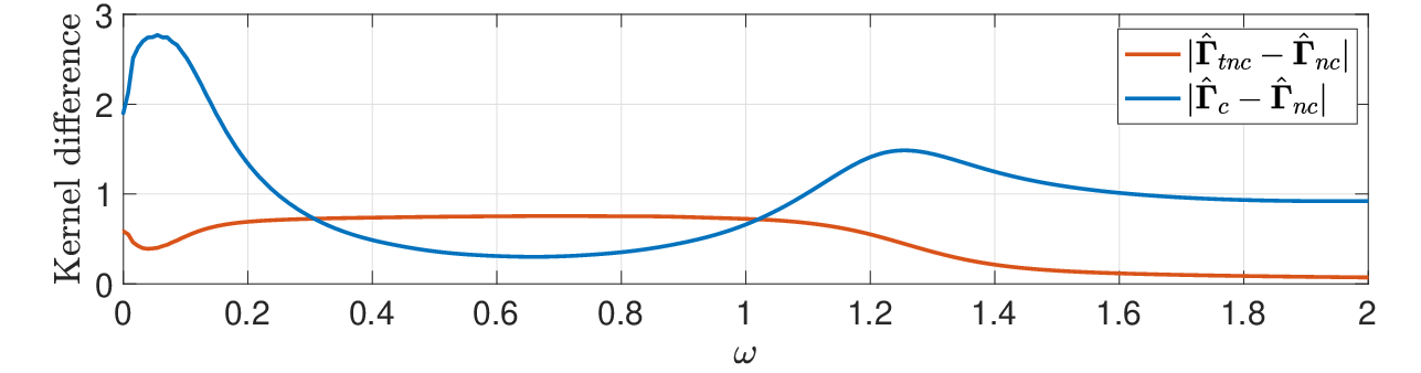
Figure 9(d) shows that the three approaches show different trends as the actuator is moved upstream. While actuator placement has a negligible influence on the non-causal control, it significantly affects the TNC control, leading to an increase in the target energy for some configurations. Causal control, on the other hand, remains efficient even when located upstream of the sensor, with the reduction in the PSD degraded by only when the actuator is located approximately 4.5 step heights upstream of the sensor.
Two different effects can explain these observations. Structures that emerge from the upstream disturbances can have significant coherence lengths, of the order of two convective time units, as later reported in figure 15. This coherence length allows the sensor to partially estimate their upstream components, which can thus be cancelled by the actuator. It is speculated that a similar mechanism is responsible for the control of a jet (a convectively unstable flow, as the present example) using downstream sensors obtained by [74] and [75]. An extreme example is when the flow is excited with a harmonic, rank-1, forcing: forces and flow response have infinite coherence lengths, and can thus be estimated and controlled based on only a few sensor readings, from which amplitudes and phases are extracted.
Another possible mechanism is the exploration of different control approaches by the causal control. As the flow studied here is incompressible, the actuation has an instantaneous, although possibly small, effect throughout the flow. This response is typically negligible for the non-causal control, which favours more effective mechanisms, but may be the only one available for the causal control when the actuator is located far upstream and exploited if low actuation penalties are used. This interpretation is supported by the dotted lines in figure 9, where the actuation penalty was drastically reduced. For upstream actuators, a significant reduction of the targets PSDs is observed for the causal control, but a small effect is observed for the non-causal control. Actuator placements upstream of the sensors tend to be less robust to unmodelled dynamics [34], and it is a configuration that is typically not used for amplifier flows [25]. Thus, upstream actuators are not further investigated in this work.
4.1.2 Control with multiple sensors
[68] reported higher perturbation reductions for a similar control configuration than those obtained here using a single sensor and actuator. However, the cited work considered only rank-1 disturbances. The present work deals with a more complex forcing scenario, with several waves exciting the Kelvin-Helmholtz instability. The identification of such multiple waves invariably requires multiple sensors; we thus explore this scenario. Four additional time-domain solutions were necessary for the results presented next, corresponding to adjoint-direct systems for the added sensors, the top and bottom circles in figure 7.
Figure 11 shows the expected target energy using the three sensors. A comparison with results obtained using one sensor identifies two trends: (i) lower target PSDs are observed, indicating that the additional sensors are indeed necessary to identify the multiple incoming waves and to accurately estimate the target readings; (ii) a larger distance between the actuator and the sensors is required for TNC to reproduce the optimal control strategies. Comparing the kernels when using one and three sensors in figure 12, it can be seen that non-causal control for three sensors is more “spread” in , and thus has more signal content for . It is then expected that its truncation leads to a more significant degradation of the control.

4.1.3 Full-rank target control
From figures 9 and 11, we conclude that the actuator should be located shortly downstream of the sensors. With sensor and actuator placements defined, control kernels for full-rank targets are constructed. This required that the following additional time-domain solutions be performed: the last equation in the sensor direct-adjoint-direct problem for each of the sensors, and the full direct-adjoint system for each actuator. In total nine additional time-domain solutions were used.
Figure 13 compares the control kernel for a rank-1 and full-rank . The close match between the two kernels indicates that downstream of the step the problem can be well approximated by a rank-1 model, and that the high-rank behaviour of the problem is indeed restricted to the receptivity of the Kelvin-Helmholtz modes to channel disturbances. This scenario is further supported by results presented in figure 14, where flow snapshots and time-series for the perturbation norm are shown for several configurations of the sensor, actuators, and targets. Control designed for full-rank targets and multiple actuators do lead to perturbation energy reduction, but the biggest improvement is provided by the use of multiple sensors.


4.2 Adjoint-less and empirical application
Here we illustrate a data-driven application of the proposed method. The necessary data can be obtained from experimental setups, from numerical solutions of the non-linear problem, or from the direct linearized problem disturbed by stochastic forcing. We focus here on the latter scenario, with the use of a single sensor and target. The generalization to more complex configurations, with more sensors, actuators, and targets, is straightforward. From sensor and target time series, the auto-correlation and cross-correlations are computed in the time domain. As previously described in § 2, (64), the terms and are equivalent to the corresponding CSDs.
Figure 15 compares estimates of and , obtained “empirically”, from the numerical experiment with different data lengths, and “analytically”, obtained with time marching of direct and adjoint equations. The resulting control kernels are also compared. Convergence trends are shown using the error, defined as
| (67) |
where the norm is used. The terms and indicate, respectively, the empirical and analytical terms, with similar expressions for the other terms. The trends suggest convergence rates scaling with , where is the time-series length used to estimate and .
Although significantly more expensive, and typically less accurate than results obtained with the use of adjoint solvers, the use of numerical experiments does extend the applicability of the method to virtually any scenario and solver, and also to derive control laws directly from experiments, which typically can be carried out to obtain long time series for better convergence of the required correlations. Note that if experimental data is used, sensor noise is already present in the data. However, if noise levels are small, adding a small noise may be required to better condition the factorization of .

4.3 Estimation and control of the non-linear system
Control laws using two different configurations for controlling the non-linear problem are investigated. As shown in § 4.1.2 and § 4.1.3, the control kernels for full- and low-rank targets provide similar results, and we thus focus on the latter. We consider two scenarios, one using one sensor, one actuator, and one target, and another using three of each. Although including statistics of the nonlinear terms within in the nonlinear case would likely improve the results [41], we chose not to pursue this so that the control law remains fixed as the forcing amplitudes increase, simplifying comparisons.
A series of non-linear simulations were performed using spatially and temporally white forcing in the upstream region indicated in figure 7 with different forcing amplitudes defined by the RMS value , i.e., . For reference, leads to perturbations that reach 10-20% of the baseflow velocity at the targets, and thus is well into the non-linear regime. As the control and estimation kernels are constructed to minimize the expected value of their respective cost functionals, a comparison should be based on an ensemble of simulations. Here we assume ergodicity of the system, and the ensemble averaging is replaced by time averaging. This assumption is validated using multiple runs for some configurations. The results for the linear problem presented in this section used an outflow condition on the right-most domain, in order to properly compare the linear and non-linear systems. The estimation and control laws should be based on a linear system that represents the non-linear problem; however, for this problem, the impact of the different boundary conditions used in the linear and non-linear systems is negligible, as reported next.


For small forcing amplitudes, the dynamics are dominated by linear mechanisms, and thus it is expected that the performance of the estimation and control laws will be the same as demonstrated in the previous sections. Focusing initially on the control problem, representative snapshots of the flow and time evolution of perturbation norms for controlled and uncontrolled non-linear systems are shown in figure 16. For the lower external forcing RMS, control of the non-linear system is similar to the control of the linearized problem, but for larger amplitudes it degrades. The perturbation norm, when normalized by the forcing RMS, reduces for larger forcing amplitudes due to non-linear saturation. Estimation and control performances are measured as the non-estimated/controlled target energy fraction,
| (68) |
Figure 17 shows as a function of . Performances for the linear and the non-linear systems are equivalent when small forcing are used, but for the latter it degrades for larger forcing amplitudes. The trend is also observed in figure 18, where time-series samples of a target for the uncontrolled problem, its causal estimation, and for the controlled problem are shown. Comparing different runs, indicated by the black dots in figure 17, it can be observed that the spread is low for the low forcing amplitudes and increases for higher amplitudes, for which the control performance is degraded.
Control and estimation performances for the linear problems are equivalent, indicating that all estimated perturbations are effectively controlled. A similar result is observed for the non-linear problem disturbed by small external forcing. Estimation deteriorates for , while control remains effective up to . As the Kelvin-Helmholtz mode amplifies upstream disturbances, small but finite disturbances are amplified and can exhibit significant non-linear dynamics. Such non-linear effects, which are not accounted for by the linear approach used, degrade estimation performance. For the controlled system, these perturbations are cancelled before they are amplified, and thus the linear assumption is valid for a larger range of external forcing amplitudes for the controlled problem.
The degraded performance of the approaches presented here when applied to the non-linear system disturbed with high-amplitude forcing is due to the saturation of the uncontrolled flow and to the violation of the assumption that the disturbances evolve linearly. From figure 16(j), comparing the normalized perturbation norm for the scenario with to those with lower values of , it can be seen that not only the perturbation norm for the controlled problem is larger, but also the norm of the uncontrolled problem is smaller. Both of these factors impact as in (68). The non-linear interactions can be treated as additional external forcing terms in the linearized equation [61, 76]. In this context, the degraded performance can be related to inadequacies of the forcing model. In particular, the non-linear interactions are not, in general, zero-mean when the linearization is performed around a baseflow, thus violating one of the assumptions used to construct the control laws. An alternative is to use a linearization around the mean flow, for which the non-linear terms are, by definition, zero mean. In previous works [40, 41] it was shown that a more representative modelling of these forcing terms can lead to significant improvements in estimation, and thus potentially to improvements in control also, for larger disturbances. Control formulations using a linearization around the mean flow may follow the methods in [69] or [71], with various mean flows used in succesive linearisations of the system as control gains are progressively increased. Integrating these approaches into the control law is beyond the scope of this study, and will be considered in future work.
5 Conclusions
Causal resolvent-based estimation and control methods based on the Wiener-Hopf framework have been presented. The approach is an extension of the non-casual resolvent-based estimation methods developed by [60] and [40] to causal estimation and control, and is obtained combining three different tools: the Wiener-regulator framework [47], matrix-free methods to obtain the action of the resolvent operator [40, 57], and numerical methods to solve matrix Wiener-Hopf problems [54]. The resulting method is directly applicable to large systems without model reduction or simplified forcing assumptions, requiring only low-rank sensor and actuator setups, which is the case in any practical configuration. Computational costs are orders-of-magnitude lower than previous approaches for full-rank systems [31]. If low-rank forcing/targets are used, inexpensive exploration of virtually any sensor/actuator configuration using only data post-processing can be obtained, allowing the optimization of sensor and actuator placements. Control of systems with high-rank forcing and targets is obtained. The ability to deal with high-rank targets avoids a possible bias of the control law towards the specific location of a given low-rank target; instead, fluctuations across the domain of interest may be minimized.
Using an open-source implementation of the proposed method, control of the flow over a backward-facing step is investigated. The flow is disturbed by high-rank forcing, making this test case considerably more challenging than a previous study that focused on rank-1 forcing [68]. Downstream of the step the flow is low rank, dominated by a Kelvin-Helmholtz instability wave, which is reflected in the fact that a control strategy is only slightly altered if targets are rank-1, rank-3, or full rank, and if one or multiple actuators are used. Considerable gains were obtained using multiple sensors, which is explained by the presence of several modes from the upstream Poiseuille-like flow and that excite the downstream Kelvin-Helmholtz waves.
Obtaining optimal controllers without model reduction circumvents possible performance losses of ROM-derived controllers when applied to the full system [30, page 349]. Moreover, the present method handles naturally complex, coloured forcing in space and time, as the forcing CSD, , can be arbitrarily specified for each frequency. This is likely crucial for the control of turbulent flows, as the behaviour of coherent structures depends strongly on how these are forced [39, 77, 40, 78, 79], but the difficulties involved in estimating and using coloured forcing models for control have hindered their use in previous applications. The method presented here, and forcing estimation methods presented in previous work [40], bridge these difficulties, allowing affordable full-rank, full-coloured controllers to be used.
This work also sheds light on the wave-cancellation behaviour of optimal control of shear flows [8], which is equivalent to the truncated-non-causal (TNC) control presented here. The approach is optimal whenever the non-causal control kernels do not rely on future information, i.e. while not designed to be causal, they are causal. This is the case for flows dominated by downstream-travelling modes, such as jets and boundary layers, provided that there is proper spacing between sensors, actuators, and targets. Reducing the distance between these, which may enhance control, generates non-causal components in the control kernel, and deteriorates the TNC approach, particularly if several sensors/actuators are used. This effect can be considerably reduced with the optimal causal control strategy developed here.
Acknowledgements
Eduardo Martini acknowledges financial support by CAPES grant 88881.190271/2018-01. Junoh Jung and Aaron Towne were supported by the Air Force Office of Scientific Research (AFOSR) grant #FA9550-20-1-0214. André V. G. Cavalieri was supported by CNPq grant 313225/2020-6.
Appendix A Wiener-Hopf problems
Analysing linear differential equations in the Fourier domain has the advantage of decoupling different frequencies for which solutions can be obtained independently. This property has been exploited in a previous study [40] to achieve optimal non-causal estimation, i.e. estimation based on both past and future sensor readings. Imposing causality, however, couples different frequencies, which must then be solved for simultaneously. The resulting equations frequently lead to Wiener-Hopf problems. We here provide a brief introduction to this class of problems and a numerical method to solve them.
A.1 Introduction
Wiener-Hopf equations appear when solving problems with restrictions applied on half domains. One example is the inversion of the half-convolution, given by
| (69) |
with considered as the unknown matrix function to be determined. The terms and are known matrix functions. In § 2, and corresponded, respectively, to the number of actuators and targets used for control, and are related to the actuator transfer functions, and to the optimal full-knowledge control. Solving (69) allows for the construction of full-knowledge control laws, as will be demonstrated later.
The frequency-domain representation of (69) is obtained by first constructing an equation valid for . Extending (69) for negative times will in general break the equality of the equation. An a priori unknown term is thus added to preserve the equality, as
| (70) |
The integral can be extended to by requiring . Similarly, requiring allows (69) and (70) to be added, leading to
| (71) |
which can be expressed in the frequency domain as
| (72) |
where
| (73) |
with similar expressions for the other variables. Although this is a single equation for two variables ( and ), the restriction that these variables be zero on different temporal half-domains ensures that the problem is well-posed.
Provided is bounded for , the requirement that is equivalent to restricting to be regular in the upper half of the complex plane. This equivalence can be observed from its inverse-Fourier transform,
| (74) |
which can be computed for by closing the contour around the upper-half plane and using the residue theorem. As for if and , the integral on the upper contour closure is zero and, as neither nor the exponential function have poles in the top-half plane, the integral is null for all . A similar argument holds for and , with the contour being closed from below. Henceforth, plus and minus subscripts are used to label functions that are regular in the upper- and lower halves of the complex frequency plane, respectively. Both frequency- and time-domain representations of functions will be used interchangeably for convenience or clarity.
Other related Wiener-Hopf problems read
| (75) |
and
| (76) |
where and .
A.2 Solving Wiener-Hopf problems
To obtain optimal causal estimation and partial-knowledge control, the Wiener-Hopf problems (22) and (40) need to be solved. In what follows, formal solutions for these equations are presented. These solutions are based on the factorization of the kernels into plus and minus components. As analytical factorization are known only for special cases, a numerical method to factorize matrix functions, tailored for functions are known only numerically, is presented.
Before proceeding, we define the two types of factorizations that will be used: additive and multiplicative. Multiplicative factorization of a matrix function reads
| (77) |
while an additive factorization reads
| (78) |
where all factors have the same size as the original matrix, and multiplicative factorizations are only defined for square matrices. To differentiate these two types of factorizations, multiplicative factors will have the subscripts applied directly to them, as in (77), and additive factors will be presented with the subscripts applied outside the parenthesis, as in (78).
These factorizations are not unique. For a multiplicative factorization as in (77), a valid factorization is constructed as and , for any constant and invertible matrix J. Likewise, new additive factorizations are obtained by respectively adding and subtracting a constant to the plus and minus factors.
Any multiplicative factorization can be used to solve Wiener-Hopf problems with the methods presented in this work, and thus we do not impose any extra condition to make it unique. However, we restrict additive factorizations to to standard factorizations [48, 80], that is
| (79) |
Note that the multiplicative factorization is also known as spectral factorization [81] in the signal processing community and is frequently expressed in terms of the Z, instead of the Fourier, transform. Typical methods to obtain this factorization are the root method, which provides an analytical factorization if the poles of the kernel are known, and the Levinson algorithm, which is based on recursion to solve a de-convolution problem. Any of these methods can in principle be used for the solution of the Wiener-Hopf problems presented here. In this work, we use the strategy proposed by [54].
A.2.1 Formal solution
To obtain a solution for (72), a multiplicative factorization of the kernel ,
| (80) |
is used. After manipulation, (72) becomes
| (81) |
Using an additive factorization of , (81) is re-written as
| (82) |
Equation (82) is in Wiener-Hopf form, with only plus (minus) functions on the left(right)-hand side. Thus, the left- and right-hand sides are analytical functions in the lower and upper complex half planes for , respectively. Solution of the Wiener-Hopf equation amounts to stating that the left- and right-hand sides are analytical continuations of each other, which allows to define a single function of that is analytical everywhere.
That each side of the equation contains only plus or minus terms suggests that each side can be solved independently, as, loosely speaking, each side is an equation for for positive/negative times only. To formalize this idea, we make use of the following assumptions,
- 1.
is bounded and positive definite,
- 2.
has no poles on the real line,
- 3.
,
and define
| (83) |
Assumption (i) guarantees that is invertible, and that does not create any poles in the right-hand side of (82). Assumption (ii) guarantees that (82) is valid on a strip around the real axis, . As the left-/right-hand-side of (82) are the analytical continuation of this strip in the upper/lower-half plane, these two functions and are regular everywhere. Since they are bounded, by Liouville’s theorem, they are also constant. Finally, assumption (iii) and the use of a standard additive factorization in (82), guarantees that the left-hand side of (82) goes to zero for , and thus that .
The solution of (72), is obtained as
| (84) | ||||
| (85) |
In this work, the assumptions (i)-(iii) are satisfied by construction. The kernels are constructed from a Hermitian quadratic form of the resolvent operator, to which a constant and Hermitian positive-definite matrix is added, thus guaranteeing assumption (i). The restriction to stable systems guarantees that the resolvent operator has no poles in the real line, and thus neither do the kernels, guaranteeing assumption (ii). Finally, as the term is a linear function of the resolvent operator, and since for , assumption (iii) is also guaranteed.
Two other Wiener-Hopf problems, (75) and (76), are used in this study. The first, which appears when solving for the full-knowledge control kernel in Appendix B, reads
| (86) |
where , , and are matrix functions. Making similar assumptions for and as the ones made for and , solutions are obtained as
| (87) |
where has a multiplicative factorisation with different convention from , given by
| (88) |
The second problem, which appears when solving for the partial knowledge optimal control kernel in § 2.3, reads
| (89) |
where now . With the same assumption as before, solutions are given by
| (90) |
A.2.2 Numerical Wiener-Hopf factorizations
An analytical expression for additive factorization reads [48]
| (91) |
with integration contours idented below or above the pole at for and functions, respectively. However, when the factors are desired numerically, additive factorizations can be easily obtained using Fourier transforms. Applying an inverse transform, the time-domain representation of the function is obtained. This representation is then split into its plus (minus) component by multiplication with a Heaviside-step function, i.e., setting to zero all values for () . A Fourier transform is then used to recover the frequency-domain representation. The function thus obtained constitutes a standard factorization: if the original function is smooth, i.e. its spectral content goes to zero for high enough frequencies, so will the factors calculated with the procedure just described.
Multiplicative factorization for scalar problems can be reduced to an additive factorization using a logarithm function to convert multiplication into addition [48, 49], with the factorization reading
| (92) |
This procedure, however, requires that the quantities commute, which is not generally the case when is a matrix. Analytical Wiener-Hopf factorizations are only known for special classes of matrices [51], and an analytical method for the factorization of general matrices is still unknown.
In this work, we use a method similar to the one described by [54] to obtain multiplicative matrix factorizations for kernels that are known numerically, rather than analytically.
The multiplicative factorization, satisfying (80), can be obtained from independent solutions of
| (93) |
as
| (94) | ||||
| (95) |
where is the size of the square matrix . That is, matrices and have vectors as columns, respectively.
To obtain solutions of (93), we divide it by , with , and integrate along a line that crosses the real axis and closes around the lower-half plane. Defining , (93) becomes a Fredholm integral equation of the second kind [54],
| (96) |
Note that (96) has only one unknown, , while (93) has two, and . The integration of the unknown term is carried out with the residue theorem, leading to , which is constant and can be arbitrarily specified. Choosing it as the canonical basis () is an obvious choice. The parameter can be arbitrarily chosen, although different values can change convergence requirements for the numerical solution of the equation. As discussed by [54], introduces an apparent singularity in the equation that, while not impacting the analytical solutions, can lead to numerical instabilities for approximate, numerical, solutions. Values close to the real axis lead to a right-hand side that has sharp variations, and thus requires finer frequency discretization to be resolved, whereas values excessively far from the real axis cause the left-hand side to have significant values on a larger domain, thus requiring the discretization of a larger frequency range. [54] suggest choosing such that it corresponds to singularities of the physical problem under study, but in the context of the problem studied here the choice is not obvious. It is thus necessary to check convergence using different values of and/or different frequency discretizations.
[54] discretized (96) to construct a matrix representing its right-hand side. The numerical solution was obtained by solving the resulting linear problem. Deformation of the integration path into the complex plane was used to improve the convergence rate of the solutions whenever the kernel had poles close to the real line. Similarly, [55] used different integration weights and collocations points to deal with such singularities. Throughout this work, we focus on kernels that are obtained numerically, and thus only available on the real frequency line. Deformation of the integration path is thus unfeasible, and convergence is obtained by refining the frequency discretization.
To solve (96), a linear problem with size has to be solved, where is the number of frequency points used, and the size of the square matrix . This approach becomes unpractical for the frequency discretization required for convergence of the results in this study. Instead, we rewrite (96) as
| (97) |
where
| (98) |
is the Hilbert transform of . Hilbert transforms can be efficiently computed numerically using fast-Fourier transforms [82], and thus the left-hand side of (97) can be obtained without the construction of the matrix that represents it. The problem is thus well suited for solutions via iterative methods, such as GMRES, used here.
As mentioned by [83], using Fourier transforms to compute Hilbert transforms can lead to significant errors at the extremities of the signal, due to the implicit assumption of periodicity. The signals need thus to be zero-padded to avoid such errors. Due to the slow decay of the term , large paddings can be necessary. Padding of 20 times the time signal has been used throughout this study.
A factorization with the order of plus and minus functions exchanged, i.e., , can be obtained via the same method using an auxiliary matrix , where ∗ represent complex conjugation. From a factorization of , the desired factorization is obtained as and .
A.2.3 Convergence


To access the convergence of the method, we compare the control kernels obtained for the Ginzburg-Landau system described in § 2.5. A normalized error is defined as
| (101) |
where is the kernel computed using the Wiener-Hopf approach and is obtained as in (53). A time interval was discretized with points spaced by , corresponding to a sampling frequency and a frequency resolution of .
The normalized error is shown in figure 19, for different values of and . The factorization scales linearly with the number of points in the frequency discretization. The linear convergence of the kernel with is a consequence of its discontinuity at : this is the convergence rate of Fourier series for discontinuous functions. Note that when actuators are close to the sensor, the discontinuity is stronger, leading to the larger errors seen when the actuator is at . The converge trend is nevertheless unaffected. Convergence with respect to the domain size is very fast, and thus has a small impact on the overall cost.
The effect of having multiple sensors and actuators on the factorization is explored in figure 20. Adding sensor/actuators leads to an increase in the required and for a given accuracy, but does not significantly affects the convergence trends. It is also seen that the cost scales linearly with the number of points used for time/frequency discretization. The increase with and is due to the need to perform matrix multiplication, which scales with the square of its size. In all scenarios, good accuracy is obtained within a few minutes on a standard notebook. Note also that this cost does not scale with the size of the system, and thus remain roughly the same for any system. When applied to complex flows, factorization is thus orders of magnitude less-costly than the time-domain solutions of the direct and adjoint problems described in § 3.1.
Appendix B The full-knowledge control problem
Complementing the optimal estimation (§ 2.2) and partial-knowledge control (§ 2.3), we here present the derivation of the optimal full-knowledge control.
Analogous to the procedure used in § 2.2, optimal control is obtained by minimizing a cost functional given by
| (102) |
Full system knowledge control implies the system state for the current time is known, from which is known can be computed. If external forcing is present, need to be updated at each time instant. An actuation, , that minimizes the cost functional can be obtained in terms of alone. Expanding terms in (102) gives
| (103) |
and differentiation with respect to leads to
| (104) |
where
| (105) |
References
- [1] Clarence W Rowley, David R. Williams, Tim Colonius, Richard M. MURRAY, and Douglas G. Macmynowski. Linear models for control of cavity flow oscillations. Journal of Fluid Mechanics, 547:317–330, 2006.
- [2] John Kim and Thomas R Bewley. A linear systems approach to flow control. Annu. Rev. Fluid Mech., 39:383–417, 2007.
- [3] Shervin Bagheri and Dan S. Henningson. Transition delay using control theory. Philosophical Transactions of the Royal Society A: Mathematical, Physical and Engineering Sciences, 369(1940):1365–1381, 2011.
- [4] Steven L. Brunton and Bernd R. Noack. Closed-Loop Turbulence Control: Progress and Challenges. Applied Mechanics Reviews, 67(050801), August 2015.
- [5] M. Luhar, A. S. Sharma, and B. J. McKeon. Opposition control within the resolvent analysis framework. Journal of Fluid Mechanics, 749:597–626, 2014.
- [6] Bo Jin, Simon J. Illingworth, and Richard D. Sandberg. Feedback control of vortex shedding using a resolvent-based modelling approach. Journal of Fluid Mechanics, 897:A26, 2020.
- [7] Kenzo Sasaki, Gilles Tissot, André V. Cavalieri, Flavio J. Silvestre, Peter Jordan, and Damien Biau. Closed-loop control of wavepackets in a free shear-flow. In 22nd AIAA/CEAS Aeroacoustics Conference, Lyon, France, May 2016. American Institute of Aeronautics and Astronautics.
- [8] Kenzo Sasaki, Pierluigi Morra, Nicoló Fabbiane, André V. G. Cavalieri, Ardeshir Hanifi, and Dan S. Henningson. On the wave-cancelling nature of boundary layer flow control. Theoretical and Computational Fluid Dynamics, 32(5):593–616, October 2018.
- [9] Pedro P. C. Brito, Pierluigi Morra, André V. G. Cavalieri, Tiago B. Araújo, Dan S. Henningson, and Ardeshir Hanifi. Experimental control of Tollmien–Schlichting waves using pressure sensors and plasma actuators. Experiments in Fluids, 62(2):32, January 2021.
- [10] Ronald E. Hanson, Kyle M. Bade, Brandt A. Belson, Philippe Lavoie, Ahmed M. Naguib, and Clarence W. Rowley. Feedback control of slowly-varying transient growth by an array of plasma actuators. Physics of Fluids, 26(2):024102, February 2014.
- [11] Kenzo Sasaki, Gilles Tissot, André V. G. Cavalieri, Flávio J. Silvestre, Peter Jordan, and Damien Biau. Closed-loop control of a free shear flow: A framework using the parabolized stability equations. Theoretical and Computational Fluid Dynamics, 32(6):765–788, December 2018.
- [12] Igor A. Maia, Peter Jordan, André V. G. Cavalieri, Eduardo Martini, Kenzo Sasaki, and Flávio J. Silvestre. Real-time reactive control of stochastic disturbances in forced turbulent jets. Physical Review Fluids, 6(12):123901, December 2021.
- [13] Nicolò Fabbiane, Onofrio Semeraro, Shervin Bagheri, and Dan S. Henningson. Adaptive and model-based control theory applied to convectively unstable flows. Applied Mechanics Reviews, 66(6), June 2014.
- [14] Bernhard Simon, Nicolò Fabbiane, Timotheus Nemitz, Shervin Bagheri, Dan S. Henningson, and Sven Grundmann. In-flight active wave cancelation with delayed-x-LMS control algorithm in a laminar boundary layer. Experiments in Fluids, 57(10):160, September 2016.
- [15] Shervin Bagheri, Dan S. Henningson, J. Hœpffner, and Peter J. Schmid. Input-Output Analysis and Control Design Applied to a Linear Model of Spatially Developing Flows. Applied Mechanics Reviews, 62(2):020803, 2009.
- [16] Thomas R. Bewley and Sharon Liu. Optimal and robust control and estimation of linear paths to transition. Journal of Fluid Mechanics, 365:305–349, 1998.
- [17] Alexandre Barbagallo, Denis Sipp, and Peter J Schmid. Closed-loop control of an open cavity flow using reduced-order models. Journal of Fluid Mechanics, 641:1–50, 2009.
- [18] Onofrio Semeraro, Shervin Bagheri, Luca Brandt, and Dan S. Henningson. Feedback control of three-dimensional optimal disturbances using reduced-order models. Journal of Fluid Mechanics, 677:63–102, 2011.
- [19] Fabien Juillet, Peter J. Schmid, and Patrick Huerre. Control of amplifier flows using subspace identification techniques. Journal of Fluid Mechanics, 725:522–565, June 2013.
- [20] Fabien Juillet, B. J. McKeon, and Peter J. Schmid. Experimental control of natural perturbations in channel flow. Journal of Fluid Mechanics, 752:296–309, 2014.
- [21] Pierluigi Morra, Kenzo Sasaki, Ardeshir Hanifi, André VG Cavalieri, and Dan S Henningson. A realizable data-driven approach to delay bypass transition with control theory. Journal of Fluid Mechanics, 883:A33, 2020.
- [22] Kenzo Sasaki, Pierluigi Morra, André V. G. Cavalieri, Ardeshir Hanifi, and Dan S. Henningson. On the role of actuation for the control of streaky structures in boundary layers. Journal of Fluid Mechanics, 883:A34, 2020.
- [23] Jeremy A. Dahan, A. S. Morgans, and S. Lardeau. Feedback control for form-drag reduction on a bluff body with a blunt trailing edge. Journal of Fluid Mechanics, 704:360–387, 2012.
- [24] Bryn Ll Jones, Peter H Heins, Eric C Kerrigan, Jonathan F Morrison, and Ati S Sharma. Modelling for robust feedback control of fluid flows. Journal of Fluid Mechanics, 769:687–722, 2015.
- [25] Peter J. Schmid and Denis Sipp. Linear control of oscillator and amplifier flows. Physical Review Fluids, 1(4):040501, August 2016.
- [26] BR Noack and H Eckelmann. Theoretical investigation of the cylinder wake with a low-dimensional Galerkin method. In Bluff-Body Wakes, Dynamics and Instabilities, pages 143–146. Springer, 1993.
- [27] Espen Åkervik, Jérôme Hœpffner, UWE Ehrenstein, and Dan S Henningson. Optimal growth, model reduction and control in a separated boundary-layer flow using global eigenmodes. Journal of Fluid Mechanics, 579:305–314, 2007.
- [28] J-N Juang and Richard S Pappa. An eigensystem realization algorithm for modal parameter identification and model reduction. Journal of guidance, control, and dynamics, 8(5):620–627, 1985.
- [29] Zhanhua Ma, Sunil Ahuja, and Clarence W Rowley. Reduced-order models for control of fluids using the eigensystem realization algorithm. Theoretical and Computational Fluid Dynamics, 25(1-4):233–247, 2011.
- [30] Karl Johan Åström and Richard M Murray. Feedback Systems: An Introduction for Scientists and Engineers. Princeton university press, 2010.
- [31] Onofrio Semeraro, Jan O. Pralits, Clarence W. Rowley, and Dan S. Henningson. Riccati-less approach for optimal control and estimation: An application to two-dimensional boundary layers. Journal of Fluid Mechanics, 731:394–417, September 2013.
- [32] Paolo Luchini and Alessandro Bottaro. Adjoint Equations in Stability Analysis. Annual Review of Fluid Mechanics, 46(1):493–517, January 2014.
- [33] C. H. Colburn, J. B. Cessna, and T. R. Bewley. State estimation in wall-bounded flow systems. Part 3. The ensemble Kalman filter. Journal of Fluid Mechanics, 682:289–303, September 2011.
- [34] Brandt A. Belson, Onofrio Semeraro, Clarence W. Rowley, and Dan S. Henningson. Feedback control of instabilities in the two-dimensional Blasius boundary layer: The role of sensors and actuators. Physics of Fluids, 25(5):054106, May 2013.
- [35] Miloš Ilak and Clarence W. Rowley. Modeling of transitional channel flow using balanced proper orthogonal decomposition. Physics of Fluids, 20(3):034103, March 2008.
- [36] Simon J. Illingworth, Aimee S. Morgans, and Clarence W. Rowley. Feedback control of flow resonances using balanced reduced-order models. Journal of Sound and Vibration, 330(8):1567–1581, 2011.
- [37] Guilherme A. Freire, André V. G. Cavalieri, Flávio J. Silvestre, A. Hanifi, and D. S. Henningson. Actuator and sensor placement for closed-loop control of convective instabilities. Theoretical and Computational Fluid Dynamics, 34(5):619–641, December 2020.
- [38] Karl J Åström and Björn Wittenmark. Computer-Controlled Systems: Theory and Design. Courier Corporation, 2013.
- [39] Mattias Chevalier, Jérôme Hœpffner, Thomas R Bewley, and Dan S Henningson. State estimation in wall-bounded flow systems. Part 2. Turbulent flows. Journal of Fluid Mechanics, 552:167–187, 2006.
- [40] Eduardo Martini, André V. G. Cavalieri, Peter Jordan, Aaron Towne, and Lutz Lesshafft. Resolvent-based optimal estimation of transitional and turbulent flows. Journal of Fluid Mechanics, 900:A2, 2020.
- [41] Filipe R. Amaral, André V.G. Cavalieri, Eduardo Martini, Peter Jordan, and Aaron Towne. Resolvent-based estimation of turbulent channel flow using wall measurements. Journal of Fluid Mechanics, 927:A17, 2021.
- [42] Norbert Wiener. The Extrapolation, Interpolation and Smoothing of Stationary Time Series with Engineering Applications: DIC Contract 6037, a Research Pursued on Behalf of the National Defense Research Council (Section D2) at the Massachusetts Institute of Technology. Massachusettes Insitute of Technology, 1942.
- [43] John F Barrett and Thomas J Moir. A unified approach to multivariable discrete-time filtering based on the Wiener-theory. Kybernetika, 23(3):177–197, 1987.
- [44] Dante Youla, Hamid Jabr, and Jr Bongiorno. Modern wiener-hopf design of optimal controllers–Part II: The multivariable case. IEEE Transactions on Automatic Control, 21(3):319–338, 1976.
- [45] MJ Grimble. Solution of the discrete-time stochastic optimal control problem in the 2-domain. International Journal of Systems Science, 10(12):1369–1390, 1979.
- [46] TJ Moir and JF Barrett. Wiener theory of digital linear-quadratic control. International Journal of Control, 49(6):2123–2155, 1989.
- [47] Fulvio Martinelli. Feedback Control of Turbulent Wall Flows. PhD thesis, PhD thesis, Politecnico di Milano, 2009.
- [48] Ben Noble. Methods Based on the Wiener-Hopf Technique for the Solution of Partial Differential Equations. Pergamon Press New York, 1959.
- [49] N Peake. On the unsteady motion of a long fluid-loaded elastic plate with mean flow. Journal of Fluid Mechanics, 507:335–366, 2004.
- [50] DG Crighton and FG Leppington. Scattering of aerodynamic noise by a semi-infinite compliant plate. Journal of Fluid Mechanics, 43(4):721–736, 1970.
- [51] V Daniele. On the factorization of Wiener-Hopf matrices in problems solvable with Hurd’s method. IEEE Transactions on Antennas and Propagation, 26(4):614–616, 1978.
- [52] AD Rawlins and WE Williams. Matrix wiener-hopf factorisation. The Quarterly Journal of Mechanics and Applied Mathematics, 34(1):1–8, 1981.
- [53] WG Tuel. Computer algorithm for spectral factorization of rational matrices. IBM Journal of Research and Development, 12(2):163–170, 1968.
- [54] V Daniele and G Lombardi. Fredholm factorization of Wiener-Hopf scalar and matrix kernels. Radio Science, 42(06):1–19, 2007.
- [55] Kendall E. Atkinson and Lawrence F. Shampine. Algorithm 876: Solving Fredholm Integral Equations of the Second Kind in Matlab. ACM Transactions on Mathematical Software, 34(4):1–20, July 2008.
- [56] Anastasia Kisil. Approximate Wiener-Hopf Factorisation with Stability Analysis. PhD thesis, University of Cambridge, 2016.
- [57] Eduardo Martini, Daniel Rodríguez, Aaron Towne, and André V.G. Cavalieri. Efficient computation of global resolvent modes. Journal of Fluid Mechanics, 919:A3, 2021.
- [58] A. Farghadan, A. Towne, E. Martini, and A. V. G. Cavalieri. A randomized time-domain algorithm for efficiently computing resolvent modes. AIAA Paper, pages 2021–2896, 2021.
- [59] Yong Li and Michael Gaster. Active control of boundary-layer instabilities. Journal of Fluid Mechanics, 550:185–205, 2006.
- [60] Aaron Towne, Adrián Lozano-Durán, and Xiang Yang. Resolvent-based estimation of space–time flow statistics. Journal of Fluid Mechanics, 883:A17, 2020.
- [61] Beverley J. McKeon and Ati S. Sharma. A critical-layer framework for turbulent pipe flow. Journal of Fluid Mechanics, 658:336–382, September 2010.
- [62] Shervin Bagheri, Luca Brandt, and Dan S Henningson. Input–output analysis, model reduction and control of the flat-plate boundary layer. Journal of Fluid Mechanics, 620:263–298, 2009.
- [63] Manfred Morari and Evanghelos Zafiriou. Robust Process Control. Morari, 1989.
- [64] Alexandre Barbagallo, Gregory Dergham, Denis Sipp, Peter J. Schmid, and Jean-Christophe Robinet. Closed-loop control of unsteadiness over a rounded backward-facing step. Journal of Fluid Mechanics, 703:326–362, July 2012.
- [65] Lutz Lesshafft. Artificial eigenmodes in truncated flow domains. Theoretical and Computational Fluid Dynamics, 32(3):245–262, June 2018.
- [66] André V. G. Cavalieri, Peter Jordan, and Lutz Lesshafft. Wave-Packet Models for Jet Dynamics and Sound Radiation. Applied Mechanics Reviews, 71(2):020802–020802–27, March 2019.
- [67] Nicolò Fabbiane, Bernhard Simon, Felix Fischer, Sven Grundmann, Shervin Bagheri, and Dan S. Henningson. On the role of adaptivity for robust laminar flow control. Journal of Fluid Mechanics, 767:R1, March 2015.
- [68] Aurelien Hervé, Denis Sipp, Peter J Schmid, and Manuel Samuelides. A physics-based approach to flow control using system identification. Journal of Fluid Mechanics, 702:26–58, 2012.
- [69] M. Högberg, T. R. Bewley, and D. S. Henningson. Relaminarization of Re=100 turbulence using gain scheduling and linear state-feedback control. Physics of Fluids, 15(11):3572–3575, November 2003.
- [70] Denis Sipp and Anton Lebedev. Global stability of base and mean flows: A general approach and its applications to cylinder and open cavity flows. Journal of Fluid Mechanics, 593, December 2007.
- [71] Colin Leclercq, Fabrice Demourant, Charles Poussot-Vassal, and Denis Sipp. Linear iterative method for closed-loop control of quasiperiodic flows. Journal of Fluid Mechanics, 868:26–65, June 2019.
- [72] Paul F Fischer and Anthony T Patera. Parallel spectral element methods for the incompressible Navier-Stokes equations. In Solution of Superlarge Problems in Computational Mechanics, pages 49–65. Springer, 1989.
- [73] Paul F Fischer. Projection techniques for iterative solution of Ax= b with successive right-hand sides. Computer methods in applied mechanics and engineering, 163(1-4):193–204, 1998.
- [74] Oleg Bychkov, Georgy Faranosov, Victor Kopiev, Vladimir Kopiev, Ivan Belyaev, Ivan Moralev, and Pavel Kazansky. Plasma-based active closed-loop control of instability waves in unexcited turbulent jet. Part 1. Free jet. 25th AIAA/CEAS Aeroacoustics Conference, 2019.
- [75] Victor Kopiev, Georgy Faranosov, Vladimir A Kopiev, Oleg P Bychkov, Ivan Moralev, and Pavel Kazansky. Plasma-based active closed-loop control of instability waves in unexcited turbulent jet. Part 2. Installed jet. In 25th AIAA/CEAS Aeroacoustics Conference, page 2558, 2019.
- [76] U. Karban, B. Bugeat, E. Martini, A. Towne, A. V. G. Cavalieri, L. Lesshafft, A. Agarwal, P. Jordan, and T. Colonius. Ambiguity in mean-flow-based linear analysis. Journal of Fluid Mechanics, 900:R5, 2020.
- [77] Aaron Towne, Oliver T. Schmidt, and Tim Colonius. Spectral proper orthogonal decomposition and its relationship to dynamic mode decomposition and resolvent analysis. Journal of Fluid Mechanics, 847:821–867, July 2018.
- [78] Petrônio A. S. Nogueira, Pierluigi Morra, Eduardo Martini, André V. G. Cavalieri, and Dan S. Henningson. Forcing statistics in resolvent analysis: Application in minimal turbulent Couette flow. Journal of Fluid Mechanics, 908:A32, 2021.
- [79] Pierluigi Morra, Petrônio A. S. Nogueira, André V. G. Cavalieri, and Dan S. Henningson. The colour of forcing statistics in resolvent analyses of turbulent channel flows. Journal of Fluid Mechanics, 907:A24, 2021.
- [80] Vito G Daniele and Rodolfo Zich. The Wiener-Hopf Method in Electromagnetics. SciTech Publishing Incorporated, 2014.
- [81] Jon F Claerbout. Fundamentals of Geophysical Data Processing, volume 274. Citeseer, 1976.
- [82] Gheorghe Todoran, Rodica Holonec, and Ciprian IAKAB. Discrete hilbert transform. numeric algorithms. Acta Electrotehnica, 49(4):485–490, 2008.
- [83] Chaoying Zhou, Lihua Yang, Yingjun Liu, and Zhihua Yang. A novel method for computing the Hilbert transform with Haar multiresolution approximation. Journal of Computational and Applied Mathematics, 223(2):585–597, 2009.