Collider Signatures of Type-X 2HDM + scalar singlet dark matter at HL-LHCPreprint: HRI-RECAPP-2021-014
Abstract
As the 125 GeV Higgs becomes disfavored as a portal to the dark sector, one is motivated to look beyond the SM-Higgs sector, into extended scalar-mediated portal mechanisms. In this work we consider one interesting possibility of such extended scalar sector, namely Type X two Higgs doublet with a scalar singlet dark matter. This model with the advantage of light pseudoscalars also provides the explanation for the observed anomalous magnetic moment of muon. The dark matter phenomenology of this model is unique from the other types of two Higgs doublet models. Therefore, it is quite intriguing to look for signatures specific to this model at the collider experiments. In this work we take up the task of finding suitable final states and regions of parameters space that can be probed at the high-luminosity runs of LHC. We go beyond our rectangular cut-based approach and use Artificial Neural Network which shows remarkable improvement in terms of signal significance.
1 Introduction
There have been strong indirect evidence of the existence of dark matter(DM) in the universe from various astrophysical and cosmological observations. The most important question arises, what constitutes DM? A simplest extension of the SM particle spectrum by a scalar gauge-singlet makes a worthy candidate, while the 125 GeV Higgs acts as the portal to this DM Djouadi:2012zc; Han:2016gyy. However, such a simple extension, namely the Higgs-portal scenario, is largely disfavored, when the direct dectection bound and observed relic density are both taken into account Lopez-Honorez:2012tov; Greljo:2013wja; Fedderke:2014wda. The reason behind this is the fact that, in simple Higgs-portal scenarios, a single coupling takes part in the scattering as well as annhilation process.
A solution to this to extend the scalar sector further with additional scalar doublets Gunion:1989we; Branco:2011iw or triplets Magg:1980ut; Schechter:1980gr; Lazarides:1980nt; Mohapatra:1980yp; Cheng:1980qt; Bilenky:1980cx; Kobzarev:1980nk; Gunion:1989ci; Mukhopadhyaya:1990up; Mohapatra:1991ng; Ma:1998dx; Chaudhuri:2013xoa; Chaudhuri:2016rwo. There have been studies in the past in the context of different types of Two Higgs Doublet Models (2HDM’s) Boucenna:2011hy; Berlin:2015wwa; Bandyopadhyay:2017tlq; Dey:2019lyr, where primarily the non-standard scalar doublet acts as a portal to the dark sector. Experimental data, such as observed relic density from Planck Ade:2013zuv, direct detection bound from XENON-1T Aprile:2018dbl, Indirect detection bounds from Fermi-LAT Wang:2017dss, put strong constraints on the model parameter space.
The present study focusses on the Type X 2HDM with an additional scalar singlet. Type X 2HDM is special from various aspects. In this model, the non-standard scalar doublet couples only to the leptons and therefore, the gluon fusion or vector-boson fusion production of the non-standard (pseuso)scalars is highly suppressed. Hence, the lighter scalar states are admissible in this model, contrary to the other types of 2HDM’s. For this special feature, Type X 2HDM garners a lot of attention from the observed muon anomaly() Bennett:2006fi; Abi:2021gix; Albahri:2021ixb. It predicts the correct in certain regions of the model parameter space, which has interesting phenomenological consequence at the LHC Cao:2009as; Arhrib:2011wc; Wang:2014sda; Crivellin:2015hha; Abe:2015oca; Liu:2015oaa; Chun:2017yob; Chun:2018vsn; Chakrabarty:2018qtt; Wang:2018hnw; Iguro:2019sly; Chun:2019oix; Bandyopadhyay:2019xfb; Frank:2020smf; Chun:2020uzw; Ghosh:2020tfq; Jueid:2021avn; Ghosh:2021jeg.
On the other hand, the DM phenomenology in case of Type X 2HDM + scalar singlet is significantly different from the scenario with Type I and Type II models Dey:2019lyr. The preferential coupling of non-standard (pseudo)scalars to leptons, helps us evade direct detection bounds easily by making DM coupling with SM doublet small, while the correct relic density can also be achieved by tuning the couplings of DM with the other doublet. This feature sets Type X 2HDM apart from the other 2HDM’s in terms of DM phenomenology. Furthermore, it is possible to have substantial invisible branching fraction for heavy scalars into DM pair, which makes it a viable scenario to look for DM at the collider.
This presents us with a great opportunity to study the collider aspects of a model, which simultaneously satisfies observed as well as provides a valid DM candidate. We perform an exhaustive scan of the parameter space with right- and wrong-sign of lepton Yukawa couplings as well as decoupling and non-decoupling extended scalar sector. We first identify the regions of parameter space which are allowed by all the relevant constraints, and choose a few suitable benchmarks from the allowed region. The benchmark selection is strongly motivated by the prospect of detectibility of this scenario at the high-luminosity LHC(HL-LHC). We also consider suitable production process and final states from this perpective. We first perform a rectangular cut-based analysis on such channels and further employ Artificial Neural Network(ANN) to achieve improved results.
The plan of this paper is as follows. In Section 2, we describe the model and important aspects of it. In Section 3, we discuss the theoretical, experimental and dark matter constraints and identify the allowed parameter space. Next, we choose a few suitable benchmarks for our collider analysis in Section 4. In Section 5, we present the cut-based analyis. The improvement over the cut-based results using machine-learning techniques, namely ANN has been explored in Section 6. We summarize and conclude our analysis in Section 7.
2 Type X 2HDM with a singlet scalar
In this work, Type X 2HDM with the inclusion of a singlet scalar is considered. can act as a possible DM candidate. The interactions of DM with SM particles, as well as DM self-interaction are given in the following Lagrangian.
| (1) |
| (2) |
Here and are Higgs doublets with and is the singlet scalar of mass . Furthermore, a symmetry is postulated, under which is odd and are even. does not have any vacuum expectation value(vev).
We start with a brief discussion on the different components of one by one.
The scalar potential:
The most general SU(2) U(1)Y invariant 2HDM scalar potential is
| (3) | |||||
In general, , and can be complex. We do not consider CP-violation in the scalar sector in our work and hence all the parameters of the scalar potential are taken to be real.
In order to avoid tree-level Flavor-changing-neutral-Current (FCNC) a softly-broken symmetry is imposed on the Higgs potential implying . After electroweak symmetry breaking, both and acquire non-zero vev as follows.
| (4) |
where .
After diagonalising of the CP-even neutral scalar mass-matrix one obtains the following physical states.
The mixing angle between the CP-even scalar states is . In this work, we will assume that the corresponds to the SM-like Higgs and is the non-standard CP-even scalar. Both of these scalars can act as a portal to the dark sector.
Gauge interactions:
The gauge interactions play crucial role in various production mechanisms of non-standard scalars and therefore are worth mentioning. The covariant kinetic-energy terms of the Lagrangian, which give rise to the gauge interactions are as follows.
| (5) |
Where . The coupling strengths of two physical CP-even scalars are as follows Branco:2011iw.
is the corresponding coupling strengths of SM-Higgs.
Yukawa interactions:
The Yukawa sector plays the essential role in distinguishing between different variants of 2HDM. The different interactions between the up-, down-type quarks and leptons and two scalar doublets classify various types of 2HDM. We focus here on Type X (lepton-specific) 2HDM, where one doublet couples to up- and down-type quarks and the other doublet couples to leptons. This can be achieved by imposing the discrete symmetry on the , and .
The Yukawa Lagrangian for Type X 2HDM can be written as follows:
| (6) |
where , , and . , and are the couplings of the up-, down-type quarks and leptons with the two doublets.
Furthermore, Yukawa couplings of the 125 GeV scalar() (which can be derived in terms of the parameters of Equation 6) here may or may not have the same sign as in the SM case Han:2020zqg,
| (7) |
Here and are the 125 GeV Higgs couplings to fermions and gauge-bosons respectively, normalized by their SM values. In Type-X 2HDM, the wrong-sign Yukawa coupling can arise only in the lepton Yukawa sector, unless region is allowed. However, the magnitudes of the couplings should be close to their SM values Sirunyan:2018koj; Aad:2019mbh, a limit known as alignment-limit.
The lepton couplings and gauge couplings of the 125 GeV scalar can be written as follows:
In the alignment limit . The possibilities that emerge depending on the sign of and range of , have been discussed in detail in Ghosh:2020tfq; Dey:2021pyn. For the sake of completeness we mention the scenarios, relevant for our discussion.
For , , takes the form . and it corresponds to right-sign region.
On the other hand, for , , and moderate , takes the form . This case also corresponds to the right-sign region.
When and and , becomes negative and . This scenario gives rise to wrong-sign lepton-Yukawa coupling.
is assumed to be an extremely small positive quantity. Also, changing the sign of ) will lead to same ranges of for both RS and WS regions.
Along with RS and WS regions there are two added possibilities. One should note that either the lightest (called Scenario 1 henceforth) or the second lightest (from now on called Scenario 2) CP-even scalar is the 125 GeV Higgs boson. We consider both possibilities in our work. We call the 125 GeV scalar as and the other non-standard scalar as . We mention here that in Scenario 2, .
The main motivation of the present study is to explore DM phenomenology of this model with light (pseudo)scalars, the existence of which makes it easier to match the observed value of . It has been shown that large region is favored from this particular requirement. With increasing precision of future experiments the allowed region of parameter space is expected to shrink and it will be imperative to probe the remaining allowed region at the collider experiments.
3 Constraints and allowed parameter space
3.1 Theoretical and phenomenological constraints
The theoretical constraints comprise of vacuum stability, perturbativity and unitarity. We are currently concerned with these constraints at the electroweak state. Vacuum essentially demands positivity of the potential at sufficiently large field values, in order to achieve boundedness. It suffices to check the quartic terms of the potential, since they dominate at large field values. Therefore the stability criterion essentially puts the following constraints on the quartic couplings Deshpande:1977rw; Nie:1998yn; Drozd:2014yla.
| (8) | |||
| (9) |
If , then one needs to also satisfy
| (10) | |||
| (11) |
Perturbativity of the quartic couplings at electroweak scale implies Drozd:2014yla
| (12) | |||
| (13) |
Furthermore, tree-level unitarity of the scattering amplitudes involving the scalars and the longitudinal components of electroweak gauge bosons Arhrib:2000is; Kanemura:1993hm demands that the eigen-values of the all the relevant scattering matrices are Lee:1977yc; Lee:1977eg; Ginzburg:2005dt.
Next come experimental constraints from colliders. Electroweak precision measurements BAAK:2014gga, especially the oblique parameters Peskin:1991sw put significant constraint on Type X parameter space when considered at one-loop level, because of the addition of additional scalars. It has been shown in various works that the non-standard scalar masses should be close to each other in order to avoid the custodial SU(2) at loop level He:2001tp; Grimus:2007if; Bhattacharyya:2015nca; Erler:2019hds. The regions of parameter space has also been identified in earlier works Broggio:2014mna; Ghosh:2020tfq; Ghosh:2021jeg; Dey:2021pyn.
CMS and ATLAS data from runs I and II on the observed 125-GeV scalar have been limiting its signal strengths in various channels with increasing precision ATLAS:2016neq; CMS:2017rli; CMS:2017jkd; CMS:2017pzi; CMS:2017zyp; ATLAS-CONF-2017-045; ATLAS-CONF-2017-043. The data shows increasing agreement to the SM values of couplings and we are pushed towards the so-called alignment limit, ie, .
Lastly, the direct search for non-standard scalars with no positive result so far does constrain the parameter space rather strongly. A crucial point regarding Type X 2HDM is the fact that the production cross-section of in gluon fusion or vector boson fusion channels are suppressed by , the suppression being major in the large region of our interest. Therefore, the masses of the non-standard scalars () can in principle be small. This property makes it significantly different from other types of 2HDMs. However, stringent constraint comes from search since the coupling increases at large .
One should also keep in mind, as low mass pseudoscalars are favored from considerations, there can be significant branching ratio of the 125 GeV Higgs to a pair of pseudoscalars as long as . However, collider searches have put strong constraint on this branching fraction. In order to obey that limit the coupling between and a pair of pseudoscalars, has be extremely strong. Parameter space consistent with this constraint have been identified in Ghosh:2020tfq; Dey:2021pyn.
3.2 Muon constraints
It is well-known that the observed anomalous magnetic moment of muon () can not be explained in the SM Aoyama:2020ynm; Davier:2017zfy; Keshavarzi:2018mgv; Colangelo:2018mtw; Hoferichter:2019mqg; Davier:2019can; Keshavarzi:2019abf; Kurz:2014wya; Melnikov:2003xd; Masjuan:2017tvw; Colangelo:2017fiz; Hoferichter:2018kwz; Gerardin:2019vio; Bijnens:2019ghy; Colangelo:2019uex; Colangelo:2014qya; Blum:2019ugy; Aoyama:2012wk; Czarnecki:2002nt; Aoyama:2019ryr; Gnendiger:2013pva; Zyla:2020zbs. There are models where additional contribution to can be achieved and therefore, are of significant importance. Type X 2HDM, is one such model which can provide correct in certain regions of parameter space. However, the current precise experimental measurements of Bennett:2006fi; Abi:2021gix; Albahri:2021ixb constrain the model parameter space to a large extent. The details of in the context of Type X 2HDM have been performed in various studies Cao:2009as; Arhrib:2011wc; Wang:2014sda; Crivellin:2015hha; Abe:2015oca; Liu:2015oaa; Chun:2017yob; Chun:2018vsn; Chakrabarty:2018qtt; Wang:2018hnw; Iguro:2019sly; Chun:2019oix; Bandyopadhyay:2019xfb; Frank:2020smf; Chun:2020uzw; Ghosh:2020tfq; Jueid:2021avn; Ghosh:2021jeg. Here we would only mention that the major contribution to comes from two-loop Bar-Zee diagrams involving light-non-standard (pseudo)scalars(which are allowed in Type X 2HDM as discussed above) and -leptons. As the -lepton coupling to (pseudo)scalars increases with , the contribution also increases with . On the other hand, low masses of the non-standard scalars (especially the pseudoscalar A, since it has most enhanced coupling to the leptons in Type X 2HDM) are preferred from the observed . The allowed regions in space with the most updated constraints can be found in Ghosh:2021jeg; Dey:2021pyn.
3.3 Constraints from dark matter search and allowed parameter space
For to be considered as a thermal dark matter candidate, it has been required here to satisfy the following constraints:
- •
The thermal relic density of should not exceed the latest Planck data Ade:2013zuv at the 2 level.
- •
The -nucleon cross section should be below the current upper bound from XENON1T Aprile:2018dbl.
- •
Constraints from indirect detection experiments should be satisfied. Therefore the annihilation rate of has been consistent at the 95% confidence level with both isotropic gamma-ray distribution data and the gamma ray observations from dwarf spheroidal galaxies Ackermann:2015zua.
- •
The invisible decay of the 125-GeV scalar has been limited to 19% Sirunyan:2018owy.
We will identify the impacts of all these constraints on our model parameter space one by one. In order to obtain regions allowed by all the aforementioned constraints, we perform a scan of the parameter space. The ranges of scan for the two Types of models are as follows(Table. 1):

In Figure 1, we select the parameter space allowed by the upper bound of relic density(orange points) and plot the direct detection cross-section () as a function of . One can see that the cross-section decreases with increasing DM mass (see the analytical expression in Equation 16). We also show the upper limit from XENON-1T experiments in the same plot.


In Figure 2, we show the dependence of relic density on dark matter couplings with physical scalars( and ). The respective couplings and can be expressed in terms of the coupling parameters of the Lagrangian (see Equation 2) and as follows:
| (14) | |||
| (15) |
We can see that the relic density falls with increasing coupling strength of DM with or . That happens because the annihilation cross-section increases with increasing couplings. We also show the region allowed by direct detection bounds in the same plot(blue points). One can see that, the allowed couplings becomes further restricted when one applies direct detection bound. The interplay between the relic density and direct detection bound is very different in Type X 2HDM as compared to Type I and Type II 2HDM. In Type X 2DHM, the up- and down-type quarks couple to the particular doublet which couples to DM states with strength and the lepton couples to the doublet which has coupling with DM particles. Therefore, coupling takes part in -nucleon scattering cross-section, and is constrained by its upper limits. On the other hand, remain almost unaffected by the direct detection bounds, a scenario very different from Type II 2HDM. Furthermore, the coupling which governs the annihilation of DM pair into final states can be adjusted in order to achieve the observed relic density. It is not possible in Type I case, since in that case same coupling takes part in relic density and direct detection cross-section. It is therefore clear that in Type X 2HDM it is easier to satisfy both constraints simultaneously.
In Figure 3, we show the allowed parameter space in the plane spanned by the couplings of DM with two physical scalar states, namely and . The direct detection cross-section is given in the following form.
| (16) |
Let us first examine the couplings involved in the calculation of DM-nucleon direct detection cross-section.
| (17) | |||
| (18) |
In Figure 3, we show the DM mass is shown as the color-axis. We see from Equation 16 that the direct detection decreases with DM mass . Also, the upper limit on direct detection cross-section becomes weaker with increasing . Therefore, larger regions get allowed for higher DM masses, which is apparent from the color distribution in Figure 3.
In the right-sign case when and , that implies and . When and are of opposite sign, and have to be of same sign to ensure cancellation between the two terms in Equation 16 and a small value of direct detection cross-section can be achieved. On the other hand, right-sign is also possible when and , which implies and . Here too, the opposite sign between and will ensure same sign between and . We can see this correlation in Figure 3(left).
The wrong-sign is possible only when and . This indicates and . Therefore the aforementioned cancellation is possible only when and are of opposite sign. We can see this behavior from Figure 3(right).
One should also take into account the indirect detection constraints on the parameter space. The major annihilation channels for DM pair are when these channels are kinematically feasible. When DM mass is small and these annihilations are not available, becomes the major channel. Therefore, the major constraint comes from indirect search from DM in the final state, especially in the low mass () region. In Figure 4, we show the annihilation cross-section of as a function of . We also show the upper limit coming from Fermi-LAT experiments in this annihilation channel, and the allowed parameter space can thus be identified.


In Figure 4, we show the distribution of annihilation cross-section for both Scenario 1(left) and 2(right). One can see that the region where (green points), the upper limit from annihilation channel constrain the parameter space significantly. One should note that, in Scenario 2, the constraints are relaxed compared to Scenario 1. The reason is the following. In Scenario 2, and are light. Therefore, even when , it is still possible that DM mass will annihilate into lighter or final states. We should mention here that while calculating the annihilation cross-section we have scaled each contribution with their relative contribution to the DM density. In this spirit, the factor in Figure 4, is the ratio of the relic density in this model with particular set of parameters and the total observed relic density of the universe ().
It is very obvious that the coupling of the 125 GeV scalar to a pair of DM() plays a crucial role in determining the branching ratio BR(. This branching ratio is highly constrained by experimental searches and the the upper limit on this is found to be 19% Sirunyan:2018owy. This upper limit in turn puts a cut-off on the coupling . In Figure 5, we plot the dependence of BR(), where is the 125 GeV scalar.
4 Selection of benchmark
Our focus in this work is to probe the aforementioned scenario and its interesting parameter space at the future colliders. For this purpose we need to select a few representative benchmarks which satisfy all the theoretical, experimental and observational constraints. The preceding discussion helps us identify allowed regions in this context. On the other hand, another crucial requirement in this regard is to select regions of parameter space which can be probed with best possible significance at the earlier runs of HL-LHC. In Type X 2HDM, the quark couplings to the non-standard scalar states () are suppressed. Therefore, the prominent production mechanism in a proton-proton collider will be via Drell-Yan process. Therefore, we will focus on Drell-Yan production of non-standard scalars, which is precisely determined by the gauge couplings. Secondly, the other important factor is the branching ratio(BR) of the non-standard CP-even scalar to a pair of DM particles, since the only way we can get DM in the final state at tree-level is via the decay of . We will first try to concentrate on the BR() in various regions of parameter space of the model.
It is obvious that to get a large BR() we must consider a large value of which controls the coupling of DM pair to our non-standard CP-even scalar . However, , and also play a crucial role here. It is discussed earlier that to satisfy observed in Type-X 2HDM, we need a moderate to large value, which enhances the branching fraction of in this model. On the other hand, for Scenario 1, where can be large, BR() can become the major decay channel of .


In Figure 6 and Figure 7, we can see the dependence of BR( on and where all other parameter are marginalized for Scenario 1 and Scenario 2. We can see that WS and RS cases are slightly different from each other. For Scenario 1,(Figure 6), in the RS domain we can get a very large BR( in certain regions with moderate , while satisfying relic as well as direct detection constraints, which can not be attained for WS domain. In WS case, in order to satisfy XENON1T bound, one can achieve only moderate BR() for in the range 25 to 50. Both in WS and RS, at very large we end up with very low BR().
On the other hand, in Scenario 2, WS and RS cases show different behavior than Scenario 1. Here we can see in Figure 7, in WS domain we can achieve a very large BR() , with moderate but in RS cases we can achieve upto 70% BR.
Next, we concentrate on dependence of BR() on mass of DM particle . We can see that for Scenario 1, to get large to moderate BR() has to be small. As can be large in this case, decay mode will open. Therefore, to increase the BR(), one has to increase the available phase space, ie. small will be favored. In Scenario 2, the mass of GeV, available phase space for is already small, therefore we can get a moderate to large BR(). However, RS case with large BR() is restricted from direct detection bound as mentioned earlier.


In the Figure 8, we can see the dependence of branchings of heavy Higgs decay in major channels with . For Scenario 1, we choose relevant parameters such as = 0.999, = = 300.0 GeV, = GeV, =20.0 GeV, . On the other hand, for Scenario 2, we choose = 0.999, = = 104.0 GeV, = GeV, = 20.0 GeV. We can see that for scenario 1, as can decay to pair, at moderate BR() becomes the dominant channel with 50% BR. However, BR() decreases with increasing and BR() starts to increase. These two decay modes share 50% BR among themselves at very large . We can also see that BR() decreases with . For Scenario 2, we see similar pattern. However, in this particular case, has no on-shell decay to final state, the contest is mostly between and final states. The former increases with whereas the latter decreases in large region.
In Figure 9, we can see the dependence of branching fractions on , with two different values. For Scenario 1, we can see that as increases, BR() increases and branching fractions to other two major decay channels, and decrease. On the other hand, for Scenario 2, as is almost fixed at a low value, the branching ratios in all possible channels remain more or less fixed in this region.
Considering all kind of dependencies of BR(), we choose six benchmark points (BP’s) from different regions of parameter space. For Scenario 1 and Scenario 2 we listed them in Table 2 and Table 3 respectively.
| BP1 | BP2 | BP3 | |
| in GeV | 200.0 | 259.13 | 153.865 |
| in GeV | 80.0 | 11.8517 | 69.0 |
| in GeV | 240.89 | 257.904 | 195.0 |
| in GeV2 | 525.965789 | 3197.1 | 347.8535 |
| in GeV | 70.0 | 100.0 | 30.5 |
| -0.00202 | -0.02751 | -0.00272 | |
| 11.574 | 12.0275 | 12.5027 | |
| 76.0 | 20.9107 | 68.0 | |
| 0.9996 | 0.993964 | 0.999996 | |
| -1.14932972 | -1.292301198257 | 0.8076599172 | |
| 6.734168% | 32.3% | 24.8% | |
| 59.87% | 5.33% | 73.89% | |
| 7.24 | 1.16 | 6.71 | |
| in | 8.214 | 1.038 | 1.396 |
For Scenario 1, we choose three benchmarks (see Table 2). BP1 represents WS Yukawa with , while BP2 has WS Yukawa with . BP3 represents RS Yukawa with . The justification behind such choices, come from the theoretical, and collider constraints along with the observed anomaly. Notably, observed muon anomaly favors large especially for . Large region implies large BR() and reduced BR(). Therefore as discussed earlier, for this scenario, in WS cases, we can not get substantial BR in channel. From Figure 6 we can see that at close to 76(BP1) and 21(BP2), we can only have low BR if we have to satisfy all constraints. On the other hand, for RS cases we can in principle have comparatively large BR. However, due to large in case of BP3, BR(.
| BP4 | BP5 | BP6 | |
| in GeV | 117.409 | 93.6073 | 121.446 |
| in GeV | 67.0 | 25.0 | 64.0 |
| in GeV | 167.0 | 135.0 | 171.0 |
| in GeV2 | 196.796761 | 282.655697 | 216.79898 |
| 40.0 | 6.0 | 50.5 | |
| -0.00254 | -0.00396 | -0.00266 | |
| 12.3745 | 3.804 | 12.3027 | |
| 70.0 | 31.0 | 68.0 | |
| -0.00141421 | 0.00447212477 | -0.0316188235075 | |
| 0.901003399 | 1.138614482 | -1.14940501 | |
| 28.2% | 67.3% | 24.0% | |
| 90.89% | 63.41% | 86.21% | |
| 9.59 | 1.88 | 3.78 | |
| in | 1.704 | 4.106 | 8.351 |
Similarly for Scenario 2, three benchmarks are chosen(see Table 3). We choose BP4 with RS Yukawa and , BP5 with RS Yukawa and and BP6 with WS Yukawa and . Here too, our choices are guided by all relevant constraints along with the observed . As the observed favors large for , BR() is on the lower side as discussed earlier. However, in Scenario 2 is comparatively smaller and therefore channel is absent. Therefore, one can achieve considerable BR(). From Figure 7, we can see that in RS case at (BP4) we get BR 28%, while for (BP5), BR( is achieved. For WS case, with (BP6), one gets 19% BR in channel.
5 Collider Analysis : Cut-based
Having discussed all important aspects of our model and chosen our benchmarks, we proceed to perform a detailed collider analysis, in terms of probing such a scenario at the high luminosity runs of LHC. The prospect at collider experiments relies heavily on choosing the signal, ie. a suitable production mechanism as well as appropriate final states. The production of DM particle will result in significant in the final state. However in order to detect that, one essentially has to consider some visible particle in the final state which will recoil against the DM. As DM in our case couples significantly only with , we will focus on the scenario where DM pair is produced from the decay of . However, we discussed earlier, the non-standard scalars in our model couple very weakly with the quarks. Therefore, the best-suited production mechanism for in this case will be via Drell-Yan process. We will focus on the following channel in our analysis.
)
As is leptophilic in nature, especially at large , it decays into with significant branching ratio( [-0.07cm] 60%) in relevant parts of the parameter space. We have considered in this work the hadronic decay mode of (BR.
5.1 Signal and backgrounds
The signal and dominant backgrounds for our process will be discussed in detail shortly. All the signal and the backgrounds are calculated at next-to-leading order, using Madgraph@MCNLO Alwall:2014hca. For multi-jet events, MLM matching has been performed with appropriate XQCUT. We have used nn23lo1 parton distribution functions. We perform showering and hadronization via PYTHIA8 Sjostrand:2006za. Delphes-3.4.1 deFavereau:2013fsa has been used for detector simulation, with in-built Fastjet Cacciari:2006sm implementation for jet formation. We mention here that at HL-LHC, due to large increase in instantaneous luminosity, pile-up effects are expected to be significant. We have included pile-up in our analysis, assuming 140 average pile-up interactions.
Signal:
Our sought after signal will be one hard -tagged jet(hadronic or ) + . We also put a veto on -jets and hard leptons(GeV). Such final states have been searched by CMS and ATLAS in the past ATLAS:2014otc; CMS:2019bfg. We closely follow the analysis strategy of CMS:2019bfg in this work.
Backgrounds:
QCD jets faking as jets: The leading background for this channel comes from QCD multi-jet events. In this case, at least one of the light QCD jets are misidentified as a -jet. Mistag rate in this case is taken to be . The large cross-section of QCD multijet process makes the tail of this background significant. However, as there is no real source of in this case, the can arise from jet-energy mismeasurement. Suitable cuts are to be applied to reduce this background. We put a generator level cut of 50 GeV on two leading jets in order to gain statistics.
+jets: The next major background comes from +jets events. In this case there are two possibilities. Firstly, can decay into final state and thus constitute an irreducible background. On the other hand, it is also possible to get misidentified -jets from leptons of -decay. However, the rate of lepton mistagging as is really small. Furthermore, there is real source of due to neutrinos from -decay. In addition, large production cross-section of +jets background makes it challenging.
: Another crucial background with real source of is . Here too, can occur from the decay of from . In addition, light-jets from top decay can also be misidentified as . However, the aforementioned -veto and lepton-veto on the events help us control the background to a large extent.
+jets: This irreducible background has larger source of compared to +jets background, when decays into a pair of neutrinos and the possibility of getting real as well as mistagged in the final state. However, its cross-section is much smaller compared to the previously mentioned backgrounds and therefore it plays only a sub-leading role in our analysis.
Single top: Lastly, single top production can also act as a possible source of background with real source of and real or fake from top decay. But due to small cross-section, this also acts as a sub-dominant background.
5.2 Distributions
In order to suppress the aforementioned backgrounds, one is motivated to look into various kinematic observables, which can distinguish between signal and backgrounds efficiently. Thereafter, suitable cuts are to be applied on those variables. With this agenda, we first show the distributions for all signal BP’s as well as the three major backgrounds.
In Figure 10(top left), we show the distribution. QCD background has no real , and the only source of is through jet energy mismeasurement. We can see that in case of QCD multijet, peaks on the lower side. On the other hand, +jets and show significant . However, the signal BP’s lie further on the higher side of spectrum, since in that case comes from the decay of a heavy scalar . It is indeed clear that a strong cut is required to reduce the backgrounds.
Figure 10(top right) shows the transverse mass distribution() in the hadronic final state. The observable is defined as follows.
| (19) |
In case of +jets and (semileptonic) backgrounds, the is coming from the decay of . Therefore in such scenarios, the distribution will be restricted by the mass. For signals on the other hand, comes from the decay of heavy and therefore distribution for signal BP’s are shifted towards higher values. This observable also plays an important role to distinguish between the signal and backgrounds.
Figure 10(centre left), we show the of the tau-tagged jet. The signal distributions for of , tend towards higher values because from the decay of decay are boosted compared to those from decay. We should mention here that the QCD jets are generated with a 50 GeV cut and its distribution therefore peaks at a higher value. In our analysis, we demand a hard -tagged jet to enhance signal over backgrounds.
Figure 10(centre right) shows the distribution of the leading light-jet. In case of QCD or background, the leading light-jet is generated in hard process and hence has similar as that of the -tagged jet. On the other hand, in case of signals, hard recoils again the DM pair and light-jets are produced mostly via showering. The of the leading light-jet in this case is rather soft. Therefore, an upper cut-off on leading light-jet will help us distinguish between signal and QCD or backgrounds. One can see in case of +jets background, the distribution is similar to the signal case, since here too, the light-jets are produced in showering and are on the softer side.
In Figure 10(bottom left), we show the distribution between the direction of and the direction of . We can see that, in case of QCD background, the is aligned with either of the jets, and the distribution also points towards that. In case of background, shows a somewhat flat distribution. +jets distribution shows a peak at . However, and there are not exactly back to back. One can see that for signals they are mostly back to back. A cut can be applied to make an effective signal-background separation.
Lastly, in Figure 10(bottom right), we present an observable . This observable is sensitive to the polarization of . The -lepton produced from decay will be left-handed and the ones produced from decay will be right-handed from angular momentum conservation. decays to a charged pion and a neutral pion and a neutrino, via intermediate meson with 25% BR. The angular distributions of the decay products are extremely sensitive to polarization. The angular observables can be translated into energy observables and can be utilized to distinguish between left-and right-handed in the lab frame. Various such observables been pointed out in ATLAS:2012tqa; CMS:2019bfg. In this work, we consider one such observable called -imbalance defined as follows.
| (20) |
For signal with right-polarized , the distribution peaks at a larger value compared to the left-handed(+jets and ) or unpolarized (QCD fakes). This observable certainly helps us distinguish between our signal and various backgrounds.
5.3 Results
Having discussed the kinematic observables, we proceed to find a suitable cut-flow, that will significantly discriminate between signal and background.
Cut flow:
Pre-selection criteria : One hard -tagged jet, 0 -jet and 0 hard lepton
Cut1 : of -tagged jet GeV
Cut2 : GeV
Cut3 : GeV
Cut4 : of the leading light-jet GeV
Cut5 :
| Datasets | Cross-section | Pre-selection cut | Cut1 | Cut2 | Cut3 | Cut4 | Cut5 |
| BP1 | 0.5 fb | 685 | 540 | 263 | 243 | 194 | 72 |
| BP2 | 0.1 fb | 140 | 112 | 60 | 56 | 44 | 17 |
| BP3 | 5.3 fb | 5338 | 3889 | 1618 | 1482 | 1198 | 596 |
| BP4 | 16 fb | 12773 | 8645 | 3056 | 2700 | 2195 | 1296 |
| BP5 | 56.5 fb | 66598 | 39947 | 11706 | 9946 | 8349 | 2980 |
| BP6 | 11.3 fb | 14207 | 9706 | 3559 | 3160 | 2584 | 934 |
| QCD multijet | pb | 3.8 | 1.6 | 1.8 | 6 | 4.0 | 300000 |
| +jets | pb | 4.9 | 4.3 | 2.7 | 7.4 | 6.8 | 109188 |
| 106 pb | 1.9 | 7.5 | 1.2 | 279840 | 133560 | 19080 | |
| +jets | 309 fb | 219866 | 51467 | 9029 | 4931 | 3856 | 445 |
| Single top | 429 fb | 96474 | 24195 | 2445 | 566 | 360 | 26 |
The significance Cowan:2010js has been calculated using the following formula.
| (21) |
| BP1 | 0.11 |
|---|---|
| BP2 | 0.03 |
| BP3 | 0.9 |
| BP4 | 2.0 |
| BP5 | 4.5 |
| BP6 | 1.5 |
One can see that BP1 and BP2 have extremely low significance. BP1, with large suffers due to small branching ratio. BP2 on the other hand, due to moderate , can have larger BR(. But in this case is sufficiently small, so that channel opens up with large branching and channel suffers from a low branching ratio. BP3 is similar to BP1, except for the masses of the non-standard scalars and DM. Smaller masses enhance production cross-section as well as BR() and therefore yield better significance. Benchmarks in Scenario 2, have significantly higher cross-section, due to small masses of the non-standard scalars. They also get significant BR() as well as BR(), since many other possible decay modes are kinematically disallowed. BP5 fares best among all the benchmarks, due to its small masses. One can infer that, in general, Scenario 2 is much easier to probe at the collider.
6 ANN Analysis
After the cut-based analysis is done, we explore the possibility of improvements of our analysis with ANN Teodorescu:2008zzb. ANN has shown marked improvement compared to results pertaining to cut-based analyses Hultqvist:1995ibm; Field:1996rw; Bakhet:2015uca; Dey:2019lyr; Lasocha:2020ctd; Dey:2020tfq; Bhowmik:2020spw. In the present analysis signal yield is poor in general because of multiple reasons discussed above. Therefore, an efficient signal-background separation method has to be adopted. With this agenda, we use ANN and calculate the significance that can be achieved at HL-LHC. We use a python-based deep-learning library Keras keras for the analysis.
From our earlier discussion, we have identified various observables which are chosen to be the input variables or feature variables for the network. Apart from the observables discussed previously, we consider a few new observables as well. These observables were not used in the cut-based analysis, due to weak discriminating power or correlation with other observables. However, we have used them for ANN analysis. We define two such additional observables below.
| (22) |
In Equation 22, the minimization is done with respect to three hardest light jets in the final state CMS:2019bfg. This observable is used typically to reduce the QCD background where one light-jet is mistagged as and is associated with mismeasurement of jet energy. This variable does not change our result significantly while used in rectangular cut-based analysis. However, we use this observable in ANN analysis.
Another such observable is ATLAS:2012tqa. It is a variable sensitive to -polarization and is defined as follow.
| (23) |
The observable in Equation 23 is expected to be correlated with and therefore was not used in the cut-based analysis. Nevertheless, we use this in our ANN analysis. All the relevant feature variables and their definitions are listed below in Table. 6.
| Variable and Definition |
|---|
| or Transverse momentum of the -tagged jet |
| or Missing transverse momenta |
| or Transverse mass |
| of the leading light-jet |
| ie. Azimuthal angle between and |
| ie. Azimuthal angle between the leading light-jet and |
| or imbalance between decay products |
| defined in Equation 22 |
| defined in Equation 23 |
| Number of light-jets |
| Number of -tagged jets |
We have used a network with four hidden layers with activation curve relu in each of them. The batch-size is taken to be 1000 and number of epochs per batch is 100. We used 80% of the dataset for training and 20% for validation. It is important to avoid over-training of the data sample. Over-training simply means the training sample yields good accuracy but the test sample fails to achieve the similar accuracy. To avoid overtraining we introduced 20% dropout at each hidden layer.
In order to guide the network towards our signal region and to thereby ensure better training, we have applied some weak kinematical cuts, eg. GeV and GeV, GeV, on signal and background events in addition to the pre-selection criteria discussed above. We obtain 92.1%(BP1), 93.4%(BP2), 92.2%(BP3), 90.6%(BP4), 88.2%(BP5) and 90.8%(BP6) accuracy after ANN analysis. In Fig. 11, the Receiver Operating Characteristic (ROC) curve for all the benchmarks are shown.
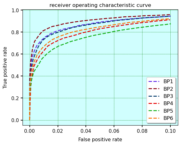
The area under curve is 0.981(BP1), 0.986(BP2), 0.98(BP3), 0.972(BP4), 0.964(BP5) and 0.974(BP6). We scan over all points on the ROC curve and choose suitable points on the curve, corresponding to each BP that yields the best signal significance. We present the signal significance for all BP’s in Table. 7.
| BP1 | 0.5 |
|---|---|
| BP2 | 0.2 |
| BP3 | 5.8 |
| BP4 | 5.2 |
| BP5 | 26.8 |
| BP6 | 8.9 |
Comparing the results of ANN in Table. 7 with that of the cut-based analysis in Table. 5 we can see that our analysis with ANN shows significant improvement for all benchmarks. However, the two BP’s in Scenario 1, namely BP1 and BP2 perform extremely poorly in cut-based as well as ANN, their signal rate being extremely small compared to the other BP’s. BP3, BP4, BP5 and BP6 on the other hand shows remarkable improvement compared to the cut-based results.
7 Summary and Conclusion
Dark matter has been one of the biggest puzzles of nature since a very long time. Its interactions with known SM fields still remain a mystery. On one hand, much talked about Higgs-portal scenario is getting constrained by data, on the other hand, the idea of an extended scalar sector acting as a portal to the dark sector is becoming more and more popular. The two Higgs doublet models are strong candidates from this viewpoint. Among various two-Higgs-doublet models, the leptophilic 2HDM or Type X 2HDM is quite interesting. It allows for low mass (pseudo)scalars unlike the other types of 2HDM’s. It also has enhanced coupling to the leptons especially at large . Owing to these particular properties, Type X 2HDM provides solution to the long standing discrepancy between the SM theoretical prediction and experimentally observed value of . It is therefore, quite motivating to study the Type X 2HDM with low mass (pseudo)scalars in detail and explore its dark matter as well as collider phenomenology. It has been observed that the dark matter phenomenology of this model is quite different from the other types of 2HDM’s, again due to its leptophilic nature. While DM coupling to one doublet gets severely restricted from the requirement of direct detection bounds, coupling to the other doublet remains free to satisfy the observed relic density of the universe. However, a pertinent question then arises, whether the regions of Type X 2HDM, that satisfy the observed muon anomaly or satisfy all the constraints from DM sector and thereby provides a legitimate portal scenario, can be probed at the collider experiments.
To answer this question, we choose suitable benchmark points from the regions that are of interest from DM phenomenology as well as observation. We select production process and specific final state involving -tagged jet + in order to ensure its detectability at the collider. Having chosen relevant kinematic observables we have achieved fair amount of signal-background separation in certain regions of the parameter space. We have also explored -polarization observables to reduce polarization sensitive electroweak background. We have found that Scenario 1, where 125 GeV Higgs is the lightest scalar, especially in the wrong-sign region becomes extremely difficult to probe in this channel even at HL-LHC. However, the situation is slightly better in the right-sign region. However, the non-decoupling scenario, where 125 GeV Higgs is the heavier scalar, has the prospect of detection at the HL-LHC. The results improve multifold when we go beyond the cut-based approach and employ the machine-learning techniques such as ANN. We would like to mention here that in Dey:2021pyn it was found that in the context of Type X 2HDM, the non-decoupling scenario is favored from the viewpoint of high scale validity too. Thus we see that, there exists an intriguing scenario, which can explain the observed muon anomaly, provides a DM candidate and a viable portal mechanism, and is also valid upto high scales and is actually testable at the HL-LHC.
8 Acknowledgement
This work was supported by funding available from the Department of Atomic Energy, Government of India, for the Regional Centre for Accelerator-based Particle Physics (RECAPP), Harish-Chandra Research Institute.
References
- (1) A. Djouadi, A. Falkowski, Y. Mambrini and J. Quevillon, Direct Detection of Higgs-Portal Dark Matter at the LHC, Eur. Phys. J. C 73 (2013) 2455, [1205.3169].
- (2) H. Han, J. M. Yang, Y. Zhang and S. Zheng, Collider Signatures of Higgs-portal Scalar Dark Matter, Phys. Lett. B 756 (2016) 109–112, [1601.06232].
- (3) L. Lopez-Honorez, T. Schwetz and J. Zupan, Higgs portal, fermionic dark matter, and a Standard Model like Higgs at 125 GeV, Phys. Lett. B 716 (2012) 179–185, [1203.2064].
- (4) A. Greljo, J. Julio, J. F. Kamenik, C. Smith and J. Zupan, Constraining Higgs mediated dark matter interactions, JHEP 11 (2013) 190, [1309.3561].
- (5) M. A. Fedderke, J.-Y. Chen, E. W. Kolb and L.-T. Wang, The Fermionic Dark Matter Higgs Portal: an effective field theory approach, JHEP 08 (2014) 122, [1404.2283].
- (6) J. F. Gunion, H. E. Haber, G. L. Kane and S. Dawson, The Higgs Hunter’s Guide, vol. 80. 2000.
- (7) G. C. Branco, P. M. Ferreira, L. Lavoura, M. N. Rebelo, M. Sher and J. P. Silva, Theory and phenomenology of two-Higgs-doublet models, Phys. Rept. 516 (2012) 1–102, [1106.0034].
- (8) M. Magg and C. Wetterich, Neutrino Mass Problem and Gauge Hierarchy, Phys. Lett. 94B (1980) 61–64.
- (9) J. Schechter and J. W. F. Valle, Neutrino Masses in SU(2) x U(1) Theories, Phys. Rev. D22 (1980) 2227.
- (10) G. Lazarides, Q. Shafi and C. Wetterich, Proton Lifetime and Fermion Masses in an SO(10) Model, Nucl. Phys. B181 (1981) 287–300.
- (11) R. N. Mohapatra and G. Senjanovic, Neutrino Masses and Mixings in Gauge Models with Spontaneous Parity Violation, Phys. Rev. D23 (1981) 165.
- (12) T. P. Cheng and L.-F. Li, Neutrino Masses, Mixings and Oscillations in SU(2) x U(1) Models of Electroweak Interactions, Phys. Rev. D22 (1980) 2860.
- (13) S. M. Bilenky, J. Hosek and S. T. Petcov, On Oscillations of Neutrinos with Dirac and Majorana Masses, Phys. Lett. 94B (1980) 495–498.
- (14) I. Yu. Kobzarev, B. V. Martemyanov, L. B. Okun and M. G. Shchepkin, THE PHENOMENOLOGY OF NEUTRINO OSCILLATIONS, Sov. J. Nucl. Phys. 32 (1980) 823.
- (15) J. F. Gunion, R. Vega and J. Wudka, Higgs triplets in the standard model, Phys. Rev. D42 (1990) 1673–1691.
- (16) B. Mukhopadhyaya, Exotic Higgs interactions and Z factories, Phys. Lett. B252 (1990) 123–126.
- (17) R. N. Mohapatra and P. B. Pal, Massive neutrinos in physics and astrophysics, World Sci. Lect. Notes Phys. 41 (1991) 1–318.
- (18) E. Ma and U. Sarkar, Neutrino masses and leptogenesis with heavy Higgs triplets, Phys. Rev. Lett. 80 (1998) 5716–5719, [hep-ph/9802445].
- (19) A. Chaudhuri, W. Grimus and B. Mukhopadhyaya, Doubly charged scalar decays in a type II seesaw scenario with two Higgs triplets, JHEP 02 (2014) 060, [1305.5761].
- (20) A. Chaudhuri and B. Mukhopadhyaya, CP -violating phase in a two Higgs triplet scenario: Some phenomenological implications, Phys. Rev. D93 (2016) 093003, [1602.07846].
- (21) M. S. Boucenna and S. Profumo, Direct and Indirect Singlet Scalar Dark Matter Detection in the Lepton-Specific two-Higgs-doublet Model, Phys. Rev. D 84 (2011) 055011, [1106.3368].
- (22) A. Berlin, S. Gori, T. Lin and L.-T. Wang, Pseudoscalar Portal Dark Matter, Phys. Rev. D 92 (2015) 015005, [1502.06000].
- (23) P. Bandyopadhyay, E. J. Chun and R. Mandal, Scalar Dark Matter in Leptophilic Two-Higgs-Doublet Model, Phys. Lett. B 779 (2018) 201–205, [1709.08581].
- (24) A. Dey, J. Lahiri and B. Mukhopadhyaya, LHC signals of a heavy doublet Higgs as dark matter portal: cut-based approach and improvement with gradient boosting and neural networks, JHEP 09 (2019) 004, [1905.02242].
- (25) Planck collaboration, P. A. R. Ade et al., Planck 2013 results. XVI. Cosmological parameters, Astron. Astrophys. 571 (2014) A16, [1303.5076].
- (26) XENON collaboration, E. Aprile et al., Dark Matter Search Results from a One Ton-Year Exposure of XENON1T, Phys. Rev. Lett. 121 (2018) 111302, [1805.12562].
- (27) L. Wang, R. Shi and X.-F. Han, Wrong sign Yukawa coupling of the 2HDM with a singlet scalar as dark matter confronted with dark matter and Higgs data, Phys. Rev. D 96 (2017) 115025, [1708.06882].
- (28) Muon g-2 collaboration, G. W. Bennett et al., Final Report of the Muon E821 Anomalous Magnetic Moment Measurement at BNL, Phys. Rev. D73 (2006) 072003, [hep-ex/0602035].
- (29) Muon g-2 collaboration, B. Abi et al., Measurement of the Positive Muon Anomalous Magnetic Moment to 0.46 ppm, Phys. Rev. Lett. 126 (2021) 141801, [2104.03281].
- (30) Muon g-2 collaboration, T. Albahri et al., Measurement of the anomalous precession frequency of the muon in the Fermilab Muon Experiment, Phys. Rev. D103 (2021) 072002, [2104.03247].
- (31) J. Cao, P. Wan, L. Wu and J. M. Yang, Lepton-Specific Two-Higgs Doublet Model: Experimental Constraints and Implication on Higgs Phenomenology, Phys. Rev. D 80 (2009) 071701, [0909.5148].
- (32) A. Arhrib, C.-W. Chiang, D. K. Ghosh and R. Santos, Two Higgs Doublet Model in light of the Standard Model search at the LHC, Phys. Rev. D 85 (2012) 115003, [1112.5527].
- (33) L. Wang and X.-F. Han, A light pseudoscalar of 2HDM confronted with muon g-2 and experimental constraints, JHEP 05 (2015) 039, [1412.4874].
- (34) A. Crivellin, J. Heeck and P. Stoffer, A perturbed lepton-specific two-Higgs-doublet model facing experimental hints for physics beyond the Standard Model, Phys. Rev. Lett. 116 (2016) 081801, [1507.07567].
- (35) T. Abe, R. Sato and K. Yagyu, Lepton-specific two Higgs doublet model as a solution of muon g 2 anomaly, JHEP 07 (2015) 064, [1504.07059].
- (36) X. Liu, L. Bian, X.-Q. Li and J. Shu, Type-III two Higgs doublet model plus a pseudoscalar confronted with , muon and dark matter, Nucl. Phys. B909 (2016) 507–524, [1508.05716].
- (37) E. J. Chun, S. Dwivedi, T. Mondal and B. Mukhopadhyaya, Reconstructing a light pseudoscalar in the Type-X Two Higgs Doublet Model, Phys. Lett. B774 (2017) 20–25, [1707.07928].
- (38) E. J. Chun, S. Dwivedi, T. Mondal, B. Mukhopadhyaya and S. K. Rai, Reconstructing heavy Higgs boson masses in a type X two-Higgs-doublet model with a light pseudoscalar particle, Phys. Rev. D98 (2018) 075008, [1807.05379].
- (39) N. Chakrabarty, C.-W. Chiang, T. Ohata and K. Tsumura, Charged scalars confronting neutrino mass and muon anomaly, JHEP 12 (2018) 104, [1807.08167].
- (40) L. Wang, J. M. Yang, M. Zhang and Y. Zhang, Revisiting lepton-specific 2HDM in light of muon anomaly, Phys. Lett. B 788 (2019) 519–529, [1809.05857].
- (41) S. Iguro, Y. Omura and M. Takeuchi, Testing the 2HDM explanation of the muon g – 2 anomaly at the LHC, JHEP 11 (2019) 130, [1907.09845].
- (42) E. J. Chun, J. Kim and T. Mondal, Electron EDM and Muon anomalous magnetic moment in Two-Higgs-Doublet Models, JHEP 12 (2019) 068, [1906.00612].
- (43) P. Bandyopadhyay, E. J. Chun and R. Mandal, Phenomenology of Higgs bosons in inverse seesaw model with Type-X two Higgs doublet at the LHC, JHEP 08 (2019) 169, [1904.09494].
- (44) M. Frank and I. Saha, Muon Anomalous Magnetic Moment in Two Higgs Doublet Models with Vector-Like Leptons, 2008.11909.
- (45) J. E. Chun and T. Mondal, Explaining anomalies in two Higgs doublet model with vector-like leptons, 2009.08314.
- (46) N. Ghosh and J. Lahiri, Revisiting a generalized two-Higgs-doublet model in light of the muon anomaly and lepton flavor violating decays at the HL-LHC, Phys. Rev. D103 (2021) 055009, [2010.03590].
- (47) A. Jueid, J. Kim, S. Lee and J. Song, Type-X two Higgs doublet model in light of the muon : confronting Higgs and collider data, 2104.10175.
- (48) N. Ghosh and J. Lahiri, Generalized 2HDM with wrong-sign lepton Yukawa coupling, in light of and lepton flavor violation at the future LHC, 2103.10632.
- (49) X.-F. Han and H.-X. Wang, Revisiting wrong sign Yukawa coupling of type II two-Higgs-doublet model in light of recent LHC data, Chin. Phys. C44 (2020) 073101, [2003.06170].
- (50) CMS collaboration, A. M. Sirunyan et al., Combined measurements of Higgs boson couplings in proton–proton collisions at , Eur. Phys. J. C79 (2019) 421, [1809.10733].
- (51) ATLAS collaboration, G. Aad et al., Combined measurements of Higgs boson production and decay using up to fb-1 of proton-proton collision data at 13 TeV collected with the ATLAS experiment, Phys. Rev. D101 (2020) 012002, [1909.02845].
- (52) A. Dey, J. Lahiri and B. Mukhopadhyaya, Muon g-2 and a type-X two Higgs doublet scenario: some studies in high-scale validity, 2106.01449.
- (53) N. G. Deshpande and E. Ma, Pattern of Symmetry Breaking with Two Higgs Doublets, Phys. Rev. D18 (1978) 2574.
- (54) S. Nie and M. Sher, Vacuum stability bounds in the two Higgs doublet model, Phys. Lett. B449 (1999) 89–92, [hep-ph/9811234].
- (55) A. Drozd, B. Grzadkowski, J. F. Gunion and Y. Jiang, Extending two-Higgs-doublet models by a singlet scalar field - the Case for Dark Matter, JHEP 11 (2014) 105, [1408.2106].
- (56) A. Arhrib, Unitarity constraints on scalar parameters of the standard and two Higgs doublets model, in Workshop on Noncommutative Geometry, Superstrings and Particle Physics, 12, 2000, hep-ph/0012353.
- (57) S. Kanemura, T. Kubota and E. Takasugi, Lee-Quigg-Thacker bounds for Higgs boson masses in a two doublet model, Phys. Lett. B 313 (1993) 155–160, [hep-ph/9303263].
- (58) B. W. Lee, C. Quigg and H. B. Thacker, The Strength of Weak Interactions at Very High-Energies and the Higgs Boson Mass, Phys. Rev. Lett. 38 (1977) 883–885.
- (59) B. W. Lee, C. Quigg and H. B. Thacker, Weak Interactions at Very High-Energies: The Role of the Higgs Boson Mass, Phys. Rev. D 16 (1977) 1519.
- (60) I. F. Ginzburg and I. P. Ivanov, Tree-level unitarity constraints in the most general 2HDM, Phys. Rev. D 72 (2005) 115010, [hep-ph/0508020].
- (61) Gfitter collaboration, M. Baak, Review of electroweak fits of the SM and beyond, after the Higgs discovery – with Gfitter, PoS EPS-HEP2013 (2013) 203.
- (62) M. E. Peskin and T. Takeuchi, Estimation of oblique electroweak corrections, Phys. Rev. D 46 (1992) 381–409.
- (63) H.-J. He, N. Polonsky and S.-f. Su, Extra families, Higgs spectrum and oblique corrections, Phys. Rev. D 64 (2001) 053004, [hep-ph/0102144].
- (64) W. Grimus, L. Lavoura, O. M. Ogreid and P. Osland, A Precision constraint on multi-Higgs-doublet models, J. Phys. G 35 (2008) 075001, [0711.4022].
- (65) G. Bhattacharyya and D. Das, Scalar sector of two-Higgs-doublet models: A minireview, Pramana 87 (2016) 40, [1507.06424].
- (66) J. Erler and M. Schott, Electroweak Precision Tests of the Standard Model after the Discovery of the Higgs Boson, Prog. Part. Nucl. Phys. 106 (2019) 68–119, [1902.05142].
- (67) A. Broggio, E. J. Chun, M. Passera, K. M. Patel and S. K. Vempati, Limiting two-Higgs-doublet models, JHEP 11 (2014) 058, [1409.3199].
- (68) ATLAS, CMS collaboration, G. Aad et al., Measurements of the Higgs boson production and decay rates and constraints on its couplings from a combined ATLAS and CMS analysis of the LHC pp collision data at and 8 TeV, JHEP 08 (2016) 045, [1606.02266].
- (69) CMS collaboration, Measurements of properties of the Higgs boson in the diphoton decay channel with the full 2016 data set, .
- (70) CMS collaboration, Measurements of properties of the Higgs boson decaying into four leptons in pp collisions at sqrts = 13 TeV, .
- (71) CMS collaboration, Higgs to WW measurements with of 13 TeV proton-proton collisions, .
- (72) CMS collaboration, A. M. Sirunyan et al., Observation of the Higgs boson decay to a pair of leptons with the CMS detector, Phys. Lett. B 779 (2018) 283–316, [1708.00373].
- (73) ATLAS Collaboration collaboration, Measurements of Higgs boson properties in the diphoton decay channel with 36.1 fb-1 collision data at the center-of-mass energy of 13 TeV with the ATLAS detector, tech. rep., CERN, Geneva, Jul, 2017.
- (74) ATLAS Collaboration collaboration, Measurement of the Higgs boson coupling properties in the decay channel at = 13 TeV with the ATLAS detector, tech. rep., CERN, Geneva, Jul, 2017.
- (75) T. Aoyama et al., The anomalous magnetic moment of the muon in the Standard Model, 2006.04822.
- (76) M. Davier, A. Hoecker, B. Malaescu and Z. Zhang, Reevaluation of the hadronic vacuum polarisation contributions to the Standard Model predictions of the muon and using newest hadronic cross-section data, Eur. Phys. J. C77 (2017) 827, [1706.09436].
- (77) A. Keshavarzi, D. Nomura and T. Teubner, Muon and : a new data-based analysis, Phys. Rev. D 97 (2018) 114025, [1802.02995].
- (78) G. Colangelo, M. Hoferichter and P. Stoffer, Two-pion contribution to hadronic vacuum polarization, JHEP 02 (2019) 006, [1810.00007].
- (79) M. Hoferichter, B.-L. Hoid and B. Kubis, Three-pion contribution to hadronic vacuum polarization, JHEP 08 (2019) 137, [1907.01556].
- (80) M. Davier, A. Hoecker, B. Malaescu and Z. Zhang, A new evaluation of the hadronic vacuum polarisation contributions to the muon anomalous magnetic moment and to , Eur. Phys. J. C80 (2020) 241, [1908.00921].
- (81) A. Keshavarzi, D. Nomura and T. Teubner, of charged leptons, , and the hyperfine splitting of muonium, Phys. Rev. D 101 (2020) 014029, [1911.00367].
- (82) A. Kurz, T. Liu, P. Marquard and M. Steinhauser, Hadronic contribution to the muon anomalous magnetic moment to next-to-next-to-leading order, Phys. Lett. B 734 (2014) 144–147, [1403.6400].
- (83) K. Melnikov and A. Vainshtein, Hadronic light-by-light scattering contribution to the muon anomalous magnetic moment revisited, Phys. Rev. D 70 (2004) 113006, [hep-ph/0312226].
- (84) P. Masjuan and P. Sanchez-Puertas, Pseudoscalar-pole contribution to the : a rational approach, Phys. Rev. D 95 (2017) 054026, [1701.05829].
- (85) G. Colangelo, M. Hoferichter, M. Procura and P. Stoffer, Dispersion relation for hadronic light-by-light scattering: two-pion contributions, JHEP 04 (2017) 161, [1702.07347].
- (86) M. Hoferichter, B.-L. Hoid, B. Kubis, S. Leupold and S. P. Schneider, Dispersion relation for hadronic light-by-light scattering: pion pole, JHEP 10 (2018) 141, [1808.04823].
- (87) A. Gérardin, H. B. Meyer and A. Nyffeler, Lattice calculation of the pion transition form factor with Wilson quarks, Phys. Rev. D 100 (2019) 034520, [1903.09471].
- (88) J. Bijnens, N. Hermansson-Truedsson and A. Rodríguez-Sánchez, Short-distance constraints for the HLbL contribution to the muon anomalous magnetic moment, Phys. Lett. B 798 (2019) 134994, [1908.03331].
- (89) G. Colangelo, F. Hagelstein, M. Hoferichter, L. Laub and P. Stoffer, Longitudinal short-distance constraints for the hadronic light-by-light contribution to with large- Regge models, JHEP 03 (2020) 101, [1910.13432].
- (90) G. Colangelo, M. Hoferichter, A. Nyffeler, M. Passera and P. Stoffer, Remarks on higher-order hadronic corrections to the muon g2, Phys. Lett. B 735 (2014) 90–91, [1403.7512].
- (91) T. Blum, N. Christ, M. Hayakawa, T. Izubuchi, L. Jin, C. Jung et al., Hadronic Light-by-Light Scattering Contribution to the Muon Anomalous Magnetic Moment from Lattice QCD, Phys. Rev. Lett. 124 (2020) 132002, [1911.08123].
- (92) T. Aoyama, M. Hayakawa, T. Kinoshita and M. Nio, Complete Tenth-Order QED Contribution to the Muon g-2, Phys. Rev. Lett. 109 (2012) 111808, [1205.5370].
- (93) A. Czarnecki, W. J. Marciano and A. Vainshtein, Refinements in electroweak contributions to the muon anomalous magnetic moment, Phys. Rev. D 67 (2003) 073006, [hep-ph/0212229].
- (94) T. Aoyama, T. Kinoshita and M. Nio, Theory of the Anomalous Magnetic Moment of the Electron, Atoms 7 (2019) 28.
- (95) C. Gnendiger, D. Stöckinger and H. Stöckinger-Kim, The electroweak contributions to after the Higgs boson mass measurement, Phys. Rev. D 88 (2013) 053005, [1306.5546].
- (96) Particle Data Group collaboration, P. A. Zyla et al., Review of Particle Physics, PTEP 2020 (2020) 083C01.
- (97) Fermi-LAT collaboration, M. Ackermann et al., Searching for Dark Matter Annihilation from Milky Way Dwarf Spheroidal Galaxies with Six Years of Fermi Large Area Telescope Data, Phys. Rev. Lett. 115 (2015) 231301, [1503.02641].
- (98) CMS collaboration, A. M. Sirunyan et al., Search for invisible decays of a Higgs boson produced through vector boson fusion in proton-proton collisions at 13 TeV, Phys. Lett. B793 (2019) 520–551, [1809.05937].
- (99) J. Alwall, R. Frederix, S. Frixione, V. Hirschi, F. Maltoni, O. Mattelaer et al., The automated computation of tree-level and next-to-leading order differential cross sections, and their matching to parton shower simulations, JHEP 07 (2014) 079, [1405.0301].
- (100) T. Sjostrand, S. Mrenna and P. Z. Skands, PYTHIA 6.4 Physics and Manual, JHEP 05 (2006) 026, [hep-ph/0603175].
- (101) DELPHES 3 collaboration, J. de Favereau, C. Delaere, P. Demin, A. Giammanco, V. Lemaître, A. Mertens et al., DELPHES 3, A modular framework for fast simulation of a generic collider experiment, JHEP 02 (2014) 057, [1307.6346].
- (102) M. Cacciari, FastJet: A Code for fast clustering, and more, in 41st Rencontres de Moriond: QCD and Hadronic Interactions, pp. 487–490, 7, 2006, hep-ph/0607071.
- (103) ATLAS collaboration, G. Aad et al., Search for charged Higgs bosons decaying via in fully hadronic final states using collision data at TeV with the ATLAS detector, JHEP 03 (2015) 088, [1412.6663].
- (104) CMS collaboration, A. M. Sirunyan et al., Search for charged Higgs bosons in the H± decay channel in proton-proton collisions at 13 TeV, JHEP 07 (2019) 142, [1903.04560].
- (105) ATLAS collaboration, G. Aad et al., Measurement of polarization in decays with the ATLAS detector in pp collisions at sqrt(s) = 7 TeV, Eur. Phys. J. C 72 (2012) 2062, [1204.6720].
- (106) G. Cowan, K. Cranmer, E. Gross and O. Vitells, Asymptotic formulae for likelihood-based tests of new physics, Eur. Phys. J. C71 (2011) 1554, [1007.1727].
- (107) L. Teodorescu, Artificial neural networks in high-energy physics, in Computing. Proceedings, inverted CERN School of Computing, ICSC2005 and ICSC2006, Geneva, Switzerland, February 23-25, 2005, and March 6-8, 2006, pp. 13–22, 2008, http://doc.cern.ch/yellowrep/2008/2008-002/p13.pdf.
- (108) K. Hultqvist, R. Jacobsson and K. E. Johansson, Using a neural network in the search for the Higgs boson, DELPHI-95-61 PHYS 496, .
- (109) R. D. Field, Y. Kanev, M. Tayebnejad and P. A. Griffin, Using neural networks to enhance the Higgs boson signal at hadron colliders, Phys. Rev. D53 (1996) 2296–2308.
- (110) N. Bakhet, M. Yu. Khlopov and T. Hussein, Neural Networks Search for Charged Higgs Boson of Two Doublet Higgs Model at the Hadrons Colliders, 1507.06547.
- (111) K. Lasocha, E. Richter-Was, M. Sadowski and Z. Was, Deep Neural Network application: Higgs boson CP state mixing angle in H to tau tau decay and at LHC, 2001.00455.
- (112) A. Dey, J. Lahiri and B. Mukhopadhyaya, LHC signals of triplet scalars as dark matter portal: cut-based approach and improvement with gradient boosting and neural networks, JHEP 06 (2020) 126, [2001.09349].
- (113) D. Bhowmik, J. Lahiri, S. Bhattacharya, B. Mukhopadhyaya and R. K. Singh, The mono-Higgs + MET signal at the Large Hadron Collider: a study on the and final states, 2012.07822.
- (114) J. R. Hermans, Distributed Keras: Distributed Deep Learning with Apache Spark and Keras, CERN IT-DB, .