Reconstruction of DBI-essence dark energy with gravity and its effect on black hole and wormhole mass accretion
Abstract
In this paper, we have used the reconstructed DBI-essence dark
energy density to modify the mass accretions of black holes and
wormholes. In general, the black hole mass accretion does not
depend on the metric or local Einstein geometry. That is why we
have used a generalized mechanism by reconstructing the
DBI-essence dark energy reconstruction with gravity. We
have used some particular forms of the scale factor to analyze the
accretion phenomena. We have shown the effect of cosmic evolution
in the proper time variation of black hole mass accretion.
Finally, we have studied the validity of energy conditions and
analyzed the type I - IV singularities for our reconstructed
model.
Keyword: black hole mass accretion, DBI-essence dark energy, Reconstruction mechanism, gravity, Cosmic evolution
1 Introduction
The black hole is one of the most important results of local solutions of the Einstein equation. The evolution of the universe follows the global solution. Although there is no direct connection between the global and local solution in geometry, the mass accretion can create a link between cosmic fluid and the black hole or wormhole like local solutions.
The nature of cosmic phases depends on the cosmic fluid with which it evolves. Various modified theories have been proposed to discuss the different cosmic phases. The Einstein Hilbert action fails to discuss the accelerated expansion of the universe, which has been experimentally proven. The introduction of the modified function of Ricci scalar in Einstein action can provide the negative pressure, which in turn can give a repulsion effect. This negativity can explain inflationary solutions as well as the late-time acceleration. From the Raychaudhuri equation, it is observed that the energy conditions must have positive values for a gravitating system. However, positive energy conditions can never produce accelerated expansion in cosmology. Therefore, simple Einstein gravity geometry alone cannot discuss the accelerated expansion properly. Modified gravity models can resolve this problem with geometry modification. There are several types of modified gravity available in the literature. Most useful modifications are gravity, Gauss-Bonnet gravity or gravity, Teleparallel gravity or gravity, non-Metricity of gravity or gravity, and so on. and come from the modifications in the metric tensor and Christoffel connections. and gravity models are basically the higher-order modification of Ricci tensor in Einstein action [1, 2, 3, 4, 5, 6, 7, 8, 9, 10, 11, 12].
The accelerated expansion or expanding universe can also be explained with the exotic nature of matter and energy. The most highlighted exotic models are the dynamic dark energy models. There are three dark energy models, namely fluid, scalar field, and Holographic models. The primary requirement behind the use of these dynamics dark energy models is to resolve the vacuum energy problem or cosmic coincidence problem [7, 17, 18, 19, 20, 21].
Dirac-Born-Infeld (DBI)-essence dark energy model [13, 14, 15, 16, 17] is one of the scalar field dynamic dark energy models that are used in cosmic physics, even in string theory. There are several types of scalar field models available in the literature, viz. Quintessence model, K-essence model, Phantom field model, H-essence model, and Tachyon model. The Tachyon model is one of the most generalized scalar field models that can discuss all the cosmic phases and conditions, but it fails to bring the cosmic Brane Bulk tension. We have used this DBI-essence model of dark energy is used in our study.
All these cosmic models modify the activity of cosmic fluids, and these modifications, in turn, modify the rate of mass accretion of black holes. It was observed that the mass accretion of the black hole and wormhole strictly depends on the cosmic phases and their evolutionary scheme. Babichev et al. [22, 23] discussed the accretion of phantom DE into a Schwarzschild black hole, using the Holographic technique, and discussed that the mass of the black hole would gradually decrease to zero near the big rip singularity. Modified gravity modifies the nature of the cosmic fluid, and that is how it can also modify the rate of mass accretion of Black holes and wormholes. The reconstruction mechanism can reproduce the evolution of energy density and pressure of the cosmic system.[25, 26, 27, 28, 29, 30, 31, 32, 23, 33, 34, 35, 36, 37]
Here in this paper, we have first reconstructed the energy density and pressure of the DBI-essence Dark energy model with gravity and discussed the energy conditions of the system. This modification has been used to discuss the black hole and wormhole mass accretion. We have discussed the rate of mass accretion in the presence of different scale factors and compared the rate with different cosmic phases. We have also tried to provide some physical reason behind the nature of mass accretion.
So, the paper is structured as follows.
In sections 2 and 3, we have discussed the basics of the modified gravity and scalar field theory. Section 4 contains the coupling calculations that help us to discuss the reconstruction formalism. Sections 5 and 6 have the basics of thermodynamic energy conditions and condensed body mass accretion. In section 7, we have discussed the analysis for different scale factors and the comparison of their results. In section 8, we have finally tried to resolve the finite-time future singularities w.r.t. the scale factors, energy densities, and pressures. We have provided the details of the results in the discussion section 9 and the overall outcome of the work in section 10.
2 Overview of gravity
The study of gravity should start from its action as follows [53]
| (1) |
Here is a function of the Ricci scalar curvature , is the determinant of 4D metric and is the matter Lagrangian. The line element for the isotropic, homogeneous, and curvature free Friedmann-Robertson-Walker (FRW) model of the universe is as follows
| (2) |
where is the scale factor of the universe. So for flat FRW model, , where is the Hubble parameter. The field equation corresponding to the above action is given by
| (3) |
where is the energy-momentum tensor. Here and are respectively the energy density and pressure of the fluid and is the fluid four vector.
In the context of our work we are using the isotropic and homogeneous FRW model and its evolutionary equation to reconstruct the DBI-essence dark energy model.
3 Overview of DBI-essence model
The DBI-essence model starts from the following Lagrangian. [16]
| (4) |
Here is a Bulk Brane tension and is the potential.
From the scalar field Lagrangian, the pressure and energy density for DBI-essence model can be given as follows [16]
| (5) |
and
| (6) |
The conservation equation for any scalar field always produce the Klein-Gordon equation which gives us the dynamical nature of scalar fields. In the case of the DBI-essence model, the modified scalar field Klein-Gordan equation can be written as follows [16]
| (7) |
We assume as used in [33], where is given by .
4 Coupling between gravity and DBI-essence DE and its reconstruction
We proceed with the reconstruction of the DBI-essence model by introducing coupling between the DBI-essence model and model. In our study, modified gravity is the reconstructing system, and the DBI-essence scalar field is reconstructed. The coupled action can be written as follows [39]
| (10) |
The Field equations corresponding to the above action are as follows
| (11) |
and
| (12) |
where and represent the energy density and pressure in context of gravity. Their expressions are as follows
| (13) |
and
| (14) |
Here, prime denotes derivative w.r.t. . The energy density due to dark matter is given by
| (15) |
where is present value of the energy density. Using equations (10)- (15), the expression of the reconstructed scalar field density and pressure for the coupled system are as follows:
| (16) |
and
| (17) |
5 Overview of different types of singularities and thermodynamic energy conditions
The types of finite time singularities are given as follows [56, 57, 42]:
- •
For any finite time, if we have ; ; ,it is known as Type-I or Big Rip singularity.
- •
For any finite time, , if we have ; ; , it is Type-II or Sudden singularity.
- •
For any finite time, if we have ; ; , it is called Type III singularity. It is found in EOS of type.
- •
At any finite time, , if we have ; ; and also the Hubble parameter and its first derivative remain finite, but its higher derivatives diverge, it is Type IV singularity. This kind of singularity is found in .
The thermodynamic energy conditions can be derived from the Raychaudhuri equation. For a congruence of time-like and null-like geodesics, the Raychaudhuri equations are given in the following forms that can be also found in the following expression in [56, 57, 21]
and
,
where is the expansion factor, is the null vector, and and are the shear and rotation associated with the vector field . For attractive gravity we may write followings
and .
For our matter-fluid distribution, the energy conditions are as follows:
- i.
Null energy condition (NEC)= .
- ii.
Weak energy condition (WEC)= and .
- iii.
Strong energy condition (SEC)= and .
- iv.
Dominant energy condition (DEC)= and .
6 Overview of black Hole and Wormhole Mass accretion
We start with the study of mass accretion of black hole which is derived in [33]. The mass accretion of black holes can be written as
| (18) |
Here is the energy momentum tensor for the fluid given by . Therefore, the above equation becomes as follows
| (19) |
where is a positive constant (details can be found in [22]). Similarly, the mass accretion of wormholes can be written as follows [33]
| (20) |
We can again re-write this equation using the functional form of energy momentum tensor for wormhole, as follows
| (21) |
where is a positive constant which can be found in [42]. We will discuss the mass accretion with the reconstructed scalar field energy density and pressure for different scale factors( and are the constants to differentiate the black holes and Wormholes mass accretion). To discuss the accretion phenomena, we consider pressureless dark matter or cold dark matter i.e., in the subsequent sections.
7 Different scale factors and mass accretion analysis
We will proceed with the discussion of the application of our reconstructed system by considering four different types of scale factor. We study the simplest form of modified gravity [6] as
| (22) |
where is constant and taken as for first two scale factor and for last two scale factors.
7.1 Scale factor
According to the results of section 4 with power-law form of scale
factor [32], where are
positive constants, we can represent and .
Here removes the initial singularity and for
accelerated universe. We plot and in Figs.
1 and 2. This and can be used in equations
(14) and (15) and the variations of kinetic energy and
potential energy can be observed in figures 3 and 4.


7.1.1 Energy conditions with reconstructed DBI-essence model and effective system
We will discuss the thermodynamic energy conditions w.r.t. the scalar field energy density and pressure that are obtained for the first assumed scale factor. The graphical representations for energy conditions are shown in Figs. 5 to 7.


7.1.2 Mass accretion formalism
The basics of mass accretion has been discussed in section 6. The mass accretion of black hole and wormhole is shown graphically in in figs. 8 and 9.


7.2 Scale factor , = constant
The second scale factor is of the form , where is even power. The importance of this constant is that it resolves any past-time singularity. We can obtain the expression and by the method discussed in section 4. The variation of and can be observed graphically in figures 10 and 11.
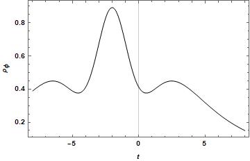
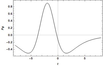
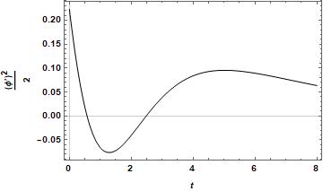
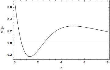
The time variation of scalar field kinetic energy and potential energy can be observed in Figs. 12 and 13.
7.2.1 Energy conditions with reconstructed DBI-essence model and effective system
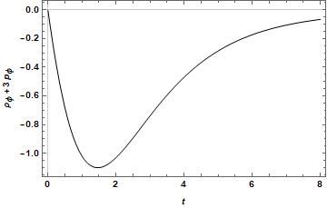
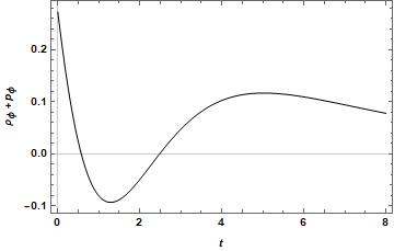
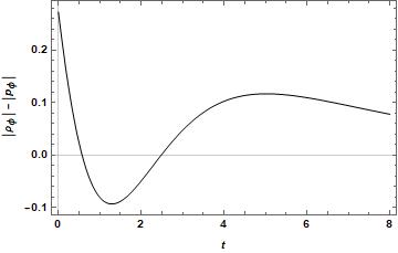
We study the thermodynamics energy conditions w.r.t. the scalar field energy density and pressure shown graphically in Fig 10 and 11 in the previous subsection.The graphical representations for energy conditions have been shown below in Figs. 14 to 16.
7.2.2 Mass accretion formalism
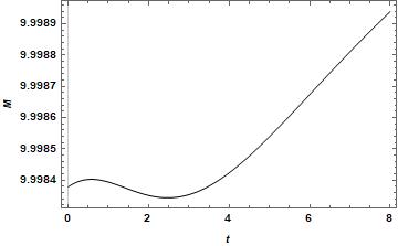
The graphical representation of mass accretion of black hole and wormhole is given in Figs. 17 and 18.
7.3 Scale factor
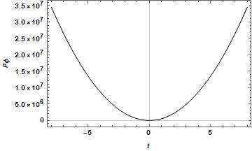
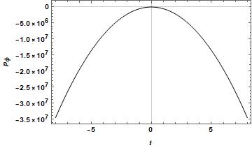
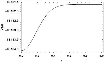
The third assumed scale factor is of the form as discussed in [32], we can derive and . The time variation of and can be observed in Figs. 19 and 20.
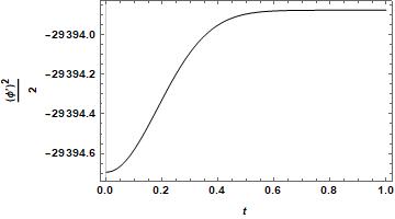
The time variation of kinetic energy and potential energy for this scale factor is shown in Figs. 21 and 22.
7.3.1 Energy conditions with reconstructed DBI-essence model and effective system
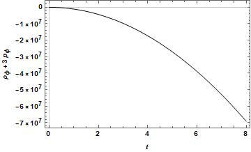
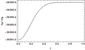
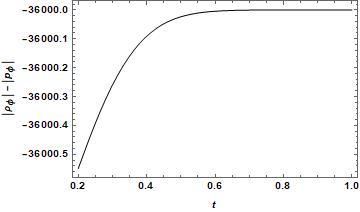
The energy conditions corresponding the the above discussed density and pressure are graphically shown in Figs. 23 to 25.
7.3.2 Mass accretion formalism
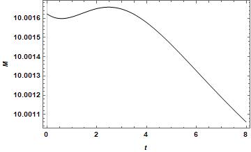
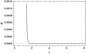
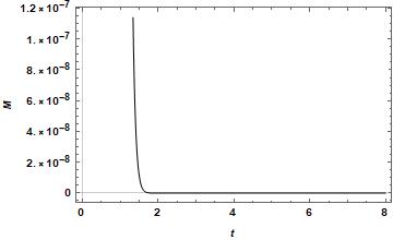
The mass accretion for the third type of scale factor is given in Figs. 26 and 27.
7.4 Scale factor
The fourth assumed scale factor is as discussed in [32], we can derive and . The time variation of and is shown in Figs. 28 and 29.


The time variation of kinetic energy and potential energy is shown in Figs. 30 and 31.


7.4.1 Energy conditions with reconstructed DBI-essence model and effective system
The graphical representations of the energy conditions corresponding to the above assumed scale factor are Figs. 32 to 34.


7.4.2 Mass accretion formalism
The variation of mass accretion of black hole and wormhole are shown in Figs. 35 and 36.


8 Removal of singularities
In section 5, we have discussed the various types of singularities that can be present in any model. In this paper, we have studied four types of scale factors. It is observed that the scalar field density and pressures of all the four types of scale factors are continuous and finite and hence there is no singularity at an initial time as well as at a future time. It is also observed that for the first scale factor in the time range and for all other scale factors in the time range we did not find any kind of singularities. Thus from fluid and geometry parameters, we can conclude that our model is free of any singularity.
9 Physical Analysis and Discussions
In this work, we have discussed four types of scale factors, along with their pictorial representation of reconstructed scalar field energy densities, pressures, kinetic energies, and potential energies. Later, we discussed energy conditions and mass accretion with respect to the reconstructed scalar field of black holes and wormholes, respectively. The detailed discussions of those results have been given in the proceeding paragraphs.
The energy densities have similar nature for the third and fourth type scale factors. Both of them have increasing nature after the point of cosmic bounce. The first type scale factor provides decreasing type energy density, whereas the second type bouncing scale factor gives some variation in nature with time. For the second type scale factor, the energy density firstly decreases with time, then after cosmic bounce, it increases with time and then again decreases. The turning points provide some phase transition whose details discussion is beyond the scope of that work.
The pictorial representations of the pressures provide exactly opposite nature of the energy densities of them. This does not happen for the second type scale factor. For the second type, the energy density and pressure have similar nature. Except for the second kind scale factor, the pressures of all other scale factors have negative values, and hence we may conclude except for the second type scale factor, all others can represent just the accelerated expansion of the universe. The pressure representation of the second scale factor can conclude that we can have a deceleration phase also somewhere after the bounce and late-time acceleration.
The nature of scalar field kinetic energy and potential energy changes with changing the scale factors, but they are surprisingly evolving in similar ways when we analyze them with fixed type scale factor. The potential of the first type scale factor provides the idea of slow roll variation. The potential for second type scale factor can provide negative results, which also proves the existence of an attractive gravity-dominated universe for some time after the cosmic bounce.
The mass accretion rate decreases for both the inflationary and bouncing type scale factors, i.e., for third and fourth type scale factors. But for first and second type scale factors, the mass accretion rate of the black hole is increasing, and for the wormhole, it is decreasing in nature.
In the analysis of energy conditions, we can find that the strong energy conditions are mostly violated. The other energy conditions are also violated except for the first and second type scale factors.
Thus, we have found a comparison between the results we found for four types of scale factors with reconstructed Dirac-Born-Infeld scalar field model with modified gravity.
10 Concluding remarks
In this paper, we have discussed the reconstructed scalar field theory in terms of the DBI-essence model. The reconstruction has been done by introducing coupling between the DBI-essence scalar field dynamic dark energy model and modified gravity, particularly gravity. We have observed late-time decreasing nature of reconstructed energy density for the first two power-law scale factors whereas an increasing nature for the last two exponential scale factors. The pressures for the first two scale factors have increasing nature and for the last two have to decrease nature.
In the analysis of mass accretion, we have found different natures for Black holes and Wormholes mass accretion for different scale factors. The variation of mass accretion for the inflationary cosmology remains similar in nature, irrespective of the nature of the scale factor.
The last two scale factors have been taken to discuss the bouncing universe and inflationary phase at the same time. The second scale factor is our assumption on power-law cosmology to resolve the initial time singularity at as well as or . The first scale factor also resolves the initial singularity but only at .
Overall, we have discussed the reconstruction mechanism and mass accretion with the discussion of energy conditions in some cosmic phases at primordial times of the universe.
Limitations of this work
The first two scale factors have been assumed, and the last two have been taken from works of Bamba et al. [32]. We have investigated the results using reconstructed scalar field theory but didn’t use any theoretical analysis on mass accretion.
Acknowledgement
The authors are thankful to the editors and reviewers for their insightful comments for valuable improvements to our paper.
References
- [1] Cuzinatto, R.R., de Melo, C.A.M., Medeiros, L.G. and Pompeia, P.J., 2015. Observational constraints on a phenomenological -model. General Relativity and Gravitation, 47(3), p.29.
- [2] Lobo, F.S., 2008. The dark side of gravity: Modified theories of gravity. arXiv preprint arXiv:0807.1640.
- [3] Moraes, P.H.R.S., Sahoo, P.K. and Pacif, S.K.J., 2020. Viability of the cosmology. General Relativity and Gravitation, 52(4), pp.1-14.
- [4] Taser, D. and Dogru, M.U., 2021. Einstein-Rosen universe with scalar field in f (R, T) theories. New Astronomy, 86, p.101575.
- [5] Singh, G.P., Bishi, B.K. and Sahoo, P.K., 2016. Cosmological constant in f (R, T) modified gravity. International Journal of Geometric Methods in Modern Physics, 13(05), p.1650058.
- [6] Debnath, P.S. and Paul, B.C., 2021. Cosmological models in R 2 gravity with hybrid expansion law. International Journal of Geometric Methods in Modern Physics, p.2150143.
- [7] Sharma, U.K. and Pradhan, A., 2018. Cosmology in modified f (R, T)-gravity theory in a variant scenario-revisited. International Journal of Geometric Methods in Modern Physics, 15(01), p.1850014.
- [8] Harko, T., Lobo, F.S., Nojiri, S.I. and Odintsov, S.D., 2011. f (R, T) gravity. Physical Review D, 84(2), p.024020.
- [9] Sotiriou, T.P. and Faraoni, V., 2010. f (R) theories of gravity. Reviews of Modern Physics, 82(1), p.451.
- [10] Sami, H., Ntahompagaze, J. and Abebe, A., 2017. Inflationary f (R) cosmologies. Universe, 3(4), p.73.
- [11] Bhattacharjee, S., Santos, J.R.L., Moraes, P.H.R.S. and Sahoo, P.K., 2020. Inflation in f (R, T) gravity. The European Physical Journal Plus, 135(7), pp.1-9.
- [12]
Sharif, M. and Nawazish, I., 2017. Cosmological analysis of scalar field models in f (R, T) gravity. The European Physical Journal C, 77(3), pp.1-13.
- [13] Sen, A., 2003. Dirac-Born-Infeld action on the tachyon kink and vortex. Physical Review D, 68(6), p.066008.
- [14] Garousi, M.R., 2000. Tachyon couplings on non-BPS D-branes and Dirac-Born-Infeld action. Nuclear Physics B, 584(1-2), pp.284-299.
- [15] Sami, M., 2007. Models of dark energy. In The Invisible Universe: Dark Matter and Dark Energy (pp. 219-256). Springer, Berlin, Heidelberg.
- [16] Martin, J. and Yamaguchi, M., 2008. DBI-essence. Physical Review D, 77(12), p.123508.
- [17]
Pal, S. and Chakraborty, S., 2019. Dynamical system analysis of a Dirac-Born-Infeld model: a center manifold perspective. General Relativity and Gravitation, 51(9), pp.1-37.
- [18] Visser, M. and Barcelo, C., 2000. Energy conditions and their cosmological implications. In Cosmo-99 (pp. 98-112).
- [19] Chattopadhyay, S., Pasqua, A. and Khurshudyan, M., 2014. New holographic reconstruction of scalar-field dark-energy models in the framework of chameleon Brans-Dicke cosmology. The European Physical Journal C, 74(9), pp.1-13.
- [20] Arora, S., Santos, J.R.L. and Sahoo, P.K., 2021. Constraining f (Q, T) gravity from energy conditions. Physics of the Dark Universe, 31, p.100790.
- [21] Sahoo, P.K., Mandal, S. and Arora, S., 2021. Energy conditions in non-minimally coupled f (R, T) gravity. Astronomische Nachrichten, 342(1-2), pp.89-95.
- [22] Babichev, E., Dokuchaev, V. and Eroshenko, Y., 2004. Black hole mass decreasing due to phantom energy accretion. Physical Review Letters, 93(2), p.021102.
- [23] Babichev, E.O., Dokuchaev, V.I. and Eroshenko, Y.N., 2005. The accretion of dark energy onto a black hole. Journal of Experimental and Theoretical Physics, 100(3), pp.528-538.
- [24] Yadav, A.K., Sahoo, P.K. and Bhardwaj, V., 2019. Bulk viscous Bianchi-I embedded cosmological model in f (R, T)= f 1 (R)+ f 2 (R) f 3 (T) gravity. Modern Physics Letters A, 34(19), p.1950145.
- [25] Sharma, L.K., Singh, B.K. and Yadav, A.K., 2020. Viability of Bianchi type V universe in gravity. International Journal of Geometric Methods in Modern Physics, 17(07), p.2050111.
- [26] Moraes, P.H.R.S. and Sahoo, P.K., 2017. The simplest non-minimal matter-geometry coupling in the f (R, T) cosmology. The European Physical Journal C, 77(7), pp.1-8.
- [27] Hulke, N., Singh, G.P., Bishi, B.K. and Singh, A., 2020. Variable Chaplygin gas cosmologies in f (R, T) gravity with particle creation. New Astronomy, 77, p.101357.
- [28] Singla, N., Gupta, M.K. and Yadav, A.K., 2020. Accelerating Model of a Flat Universe in Gravity. Gravitation and Cosmology, 26(2), pp.144-152.
- [29] Sharif, M., Rani, S. and Myrzakulov, R., 2013. Analysis of F (R, T) gravity models through energy conditions. The European Physical Journal Plus, 128(10), pp.1-11.
- [30] Debnath, U., Chattopadhyay, S., Hussain, I., Jamil, M. and Myrzakulov, R., 2012. Generalized second law of thermodynamics for FRW cosmology with power-law entropy correction. The European Physical Journal C, 72(2), pp.1-6.
- [31]
Kar, A., Sadhukhan, S. and Chattopadhyay, S., 2021. Energy conditions for inhomogeneous EOS and its thermodynamics analysis with the resolution on finite time future singularity problems. International Journal of Geometric Methods in Modern Physics, Vol. 18, No. 08, 2150131 (2021)
- [32] Bamba, K., Makarenko, A.N., Myagky, A.N. and Odintsov, S.D., 2014. Bouncing cosmology in modified Gauss-Bonnet gravity. Physics Letters B, 732, pp.349-355.
- [33] Debnath, U., 2015. Accretions of dark matter and dark energy onto (n+)-dimensional Schwarzschild black hole and Morris-Thorne wormhole. Astrophysics and Space Science, 360(2), pp.1-9.
- [34] Debnath, U., 2015. Accretion and evaporation of modified Hayward black hole. The European Physical Journal C, 75(3), pp.1-5.
- [35] Debnath, U., 2020. Accretion of Some Classes of Holographic DE onto Higher-Dimensional Schwarzschild Black Holes. Gravitation and Cosmology, 26, pp.75-81.
- [36] Jawad, A. and Shahzad, M.U., 2016. Accretion onto some well-known regular black holes. The European Physical Journal C, 76(3), pp.1-11.
- [37] Michel, F.C., 1972. Accretion of matter by condensed objects. Astrophysics and Space Science, 15(1), pp.153-160.
- [38] John, A.J., Ghosh, S.G. and Maharaj, S.D., 2013. Accretion onto a higher dimensional black hole. Physical Review D, 88(10), p.104005.
- [39] Karmakar, S., Chattopadhyay, S. and Radinschi, I., 2020. A holographic reconstruction scheme for f(R) gravity and the study of stability and thermodynamic consequences. New Astronomy, 76, p.101321.
- [40] Chattopadhyay, S. and Pasqua, A., 2013. Holographic DBI-essence dark energy via power-law solution of the scale factor. International Journal of Theoretical Physics, 52(11), pp.3945-3952.
- [41] Nojiri, S.I. and Odintsov, S.D., 2005. Inhomogeneous equation of state of the universe: Phantom era, future singularity, and crossing the phantom barrier. Physical Review D, 72(2), p.023003.
- [42] González-Díaz, P.F., 2006. Some notes on the big trip. Physics Letters B, 635(1), pp.1-6.
- [43] Kar, A., Sadhukhan, S. and Debnath, U., 2021. Condensed body mass accretion with DBI-essence dark energy and its reconstruction with f (Q) gravity. arXiv preprint arXiv:2109.10906.
- [44] Kar, A., Sadhukhan, S. and Chattopadhyay, S., 2021. Thermodynamics and energy condition analysis for Van-Der-Waals EOS without viscous cosmology. Physica Scripta. https://doi.org/10.1088/1402-4896/ac2f00
- [45] Armendariz-Picon, C., Damour, T. and Mukhanov, V.I., 1999. k-Inflation. Physics Letters B, 458(2-3), pp.209-218.
- [46] Debnath, U. and Jamil, M., 2011. Correspondence between DBI-essence and modified Chaplygin gas and the generalized second law of thermodynamics. Astrophysics and Space Science, 335(2), pp.545-552.
- [47] Armendariz-Picon, C., Mukhanov, V. and Steinhardt, P.J., 2001. Essentials of k-essence. Physical Review D, 63(10), p.103510.
- [48] Malaver, Manuel, Hamed Daei Kasmaei, Rajan Iyer, Shouvik Sadhukhan, and Alokananda Kar. ”A theoretical model of Dark Energy Stars in Einstein-Gauss-Bonnet Gravity.” arXiv preprint arXiv:2106.09520 (2021).
- [49] S. Sadhukhan, Quintessence model calculations for bulk viscous fluid and low value predictions of the coefficient of bulk viscosity.Int. J. Sci. Res. (IJSR) 9(3), 1419-1420 (2020). https://doi.org/10.21275/SR20327132301
- [50] A. Kar, S. Sadhukhan, Hamiltonian Formalism for Bianchi Type I Model for Perfect Fluid as Well as for the Fluid with Bulk and Shearing Viscosity. Basic and Applied Sciences into Next Frontiers (New Delhi Publishers, 2021) (ISBN: 978-81-948993-0-3)
- [51] A. Kar, S. Sadhukhan, Quintessence model with bulk viscosity and some predictions on the coefficient of bulk viscosity and gravitational constant, recent advancement of mathematics in science and technology (2021) (ISBN: 978-81-950475-0-5)
- [52] Myrzakulov, R., 2012. FRW cosmology in f (R, T) gravity. The European Physical Journal C, 72(11), pp.1-9.
- [53] Hans A. Buchdahl, Non-linear Lagrangians and cosmological theory, Mon.Not.Roy.Astron.Soc., 150,1 (1970).
- [54] Raychaudhuri, A., 1953. Arbitrary concentrations of matter and the Schwarzschild singularity. Physical Review, 89(2), p.417.
- [55] Raychaudhuri, A., 1952. Condensations in Expanding Cosmologic Models. Physical Review, 86(1), p.90.
- [56] Raychaudhuri, A., 1955. Relativistic cosmology. I. Physical Review, 98(4), p.1123.
- [57] Raychaudhuri, A.M.A.L.K.U.M.A.R., 1957. Relativistic and Newtonian cosmology. Zeitschrift für Astrophysik, 43, pp.161-164.
- [58] Sadhukhan, S., Kar, A. and Chattopadhay, S., 2021. Thermodynamic analysis for Non-linear system (Van-der-Waals EOS) with viscous cosmology. The European Physical Journal C, 81(10), pp.1-21.