Modelling Matrix Time Series via a Tensor CP-Decomposition

Jinyuan Chang Affiliation: Joint Laboratory of Data Science and Business Intelligence, Southwestern University of Finance and Economics, Chengdu, Sichuan 611130, China Jing He Affiliation: Joint Laboratory of Data Science and Business Intelligence, Southwestern University of Finance and Economics, Chengdu, Sichuan 611130, China Lin Yang Affiliation: Joint Laboratory of Data Science and Business Intelligence, Southwestern University of Finance and Economics, Chengdu, Sichuan 611130, China Qiwei Yao Affiliation: Department of Statistics, The London School of Economics and Political Science, London, WC2A 2AE, U.K.

Abstract

We consider to model matrix time series based on a tensor CP-decomposition. Instead of using an iterative algorithm which is the standard practice for estimating CP-decompositions, we propose a new and one-pass estimation procedure based on a generalized eigenanalysis constructed from the serial dependence structure of the underlying process. To overcome the intricacy of solving a rank-reduced generalized eigenequation, we propose a further refined approach which projects it into a lower-dimensional full-ranked eigenequation. This refined method improves significantly the finite-sample performance of the estimation. The asymptotic theory has been established under a general setting without the stationarity. It shows, for example, that all the component coefficient vectors in the CP-decomposition are estimated consistently with certain convergence rates. The proposed model and the estimation method are also illustrated with both simulated and real data; showing effective dimension-reduction in modelling and forecasting matrix time series.

Keywords: Dimension-reduction; Generalized eigenanalysis; Matrix time series; Tensor CP-decomposition.

1 Introduction

Let ${\mathbf{Y}}_{t}=(y_{i,j,t})$ be a $p\times q$ matrix time series, i.e. there are $pq$ recorded values at each time $t$ from, for example, $p$ individuals and over $q$ indices or variables, and $y_{i,j,t}$ is then the value of the $j$ -th variable on the $i$ -th individual at time $t$ . Given available observations ${\mathbf{Y}}_{1},\ldots,{\mathbf{Y}}_{n}$ , the goal is to build a dynamic model for ${\mathbf{Y}}_{t}$ and to forecast the future values ${\mathbf{Y}}_{n+\ell}$ for $\ell\geq 1$ . With moderately large $p$ and $q$ , any direct attempts based on the time series ARMA framework are unlikely to be successful due to overparametrization. We seek a low-dimensional structure via a tensor canonical polyadic (CP) decomposition. To this end, we denote by $\EuScriptBF Y$ the $p\times q\times n$ tensor with ${\mathbf{Y}}_{1},\ldots,{\mathbf{Y}}_{n}$ as its $n$ frontal slices (Kolda and Bader 2009). Then $y_{i,j,t}$ is the $(i,j,t)$ -th element of $\EuScriptBF Y$ . Conceptually we decompose $\EuScriptBF Y$ into two parts:

\EuScriptBF Y=\EuScriptBF X+\EuScriptBF E\,,

(1)

where all the dynamic structure of $\EuScriptBF Y$ is reflected by $\EuScriptBF X$ , and the frontal slices of $\EuScriptBF E\equiv({\varepsilon}_{i,j,t})$ are matrix white noise, i.e. ${\rm Cov}({\varepsilon}_{i,j,t},{\varepsilon}_{k,\ell,s})=0$ for any $t\neq s$ . The key idea is to perform a CP-decomposition for $\EuScriptBF X$ , i.e. to express it as a sum of rank one tensors (see (2) below). This effectively represents the dynamic structure of matrix process ${\mathbf{Y}}_{t}$ in terms of that of a vector process, and, hence, achieving an effective dimension-reduction in modeling the dynamic behaviour of the process.

The ‘workhorse’ method for CP-decompositions is the so-called alternative least squares (ALS) algorithm which is easy to understand and implement. See Section 3.4 of Kolda and Bader 2009 and the references therein. However it has obvious drawbacks. For example, an ALS algorithm takes many iterations to converge. It is not guaranteed to converge to the global minimum even for moderately large $p$ , $q$ or $n$ . Furthermore it also depends sensitively on the selection of the initial values. Substantial effort has been made to improve the convergence and the performance of the ALS algorithm, including, among others, Anandkumar et al. 2014, Liu et at. 2014, Colombo and Vlassis 2016, Sun at al. 2017, Sharan and Valiant 2017, Wang and Song 2017, Zhang and Xia 2018, and Han and Zhang 2021.

We propose a new and one-pass estimation procedure in this paper. The new method is inspired by Sanchez and Kowalski 1990 which transforms a CP-decomposition into a generalized eigenanalysis problem. While Sanchez and Kowalski’s approach does not require iteration, it only works for the noise-free cases with $\EuScriptBF E\equiv{\mathbf{0}}$ in (1). In contrast, our new procedure eliminates the impact of the noise by incorporating the serial dependence into the estimation. Furthermore to overcome the intricacy in solving a generalized eigenequation defined by rank-reduced matrices (see Section 7.7 of Golub and Van Loan 2013), we propose a new refined approach which projects a rank-reduced generalized eigenequation to a full-ranked lower-dimensional one which is, therefore, equivalent to a standard eigenequation. The numerical results in simulation also demonstrate the significant improvement in the finite sample performance by this refined method.

Most existing literature on matrix time series is based on the factor modelling via the Tucker decomposition; see Chen and Chen 2019, Wang et al. 2019 and Chen et al. 2020. The key difference between our approach and the Tucker decomposition based approaches is two fold. First, a Tucker decomposition represents a matrix process as a linear combination of a smaller matrix process while a CP-decomposition is more canonical in the sense that it represents a matrix process in terms of a vector process; see also the real data example in Section 5.2 below. Secondly, a Tucker decomposition entails more conventional factor models, and, therefore, we only need to identify and estimate the factor loading spaces, for which the standard factor model methods (e.g. Lam and Yao 2012, and Chang et al. 2015) are applicable. However for a CP-decomposition, we need to identify and estimate the component coefficient vectors precisely. Therefore a radically new inference procedure is required. The other approaches for modelling matrix time series include: the matrix-coefficient autoregressive models of Chen et al. 2021, and the bilinear transformation segmentation method of Han et al. 2021a. Han et al. 2021b models tensor time series also based on a CP-decomposition. But their approach is radically different from ours, as they estimate the CP-decomposition based on an iterative simultaneous orthogonalization algorithm with a warm-start initialization using the so-called composite principal component analysis for tensors; see Section 3 of Han et al. 2021b. Note that our estimation is an one-pass procedure, and no iterations are required.

The rest of the paper is organized as follows. The matrix time series model based on a CP-decomposition is presented in Section 2. Section 3 deals with the model identification and presents the newly proposed estimation procedures. The asymptotic results, including the convergence rates for the estimated component vectors in the CP-decomposition, are presented in Section 4. Numerical illustration with both simulated and real data sets is given in Section 5. All the technical proofs are relegated to the supplementary material.

Notations. For a positive integer $m$ , write $[m]=\{1,\ldots,m\}$ , and denote by ${\mathbf{I}}_{m}$ the $m\times m$ identity matrix. Let $I(\cdot)$ be the indicator function. For an $m_{1}\times m_{2}$ matrix ${\mathbf{H}}=(h_{i,j})_{m_{1}\times m_{2}}$ , let $\|{\mathbf{H}}\|_{2}$ , ${\rm rank}({\mathbf{H}})$ , $\sigma_{\min}({\mathbf{H}})$ and ${\rm vec}({\mathbf{H}})$ be, respectively, its spectral norm, its rank, its smallest singular value, and a vector obtained by stacking together the columns of ${\mathbf{H}}$ . Specifically, if $m_{2}=1$ , we use $|{\mathbf{H}}|_{2}=(\sum_{i=1}^{m_{1}}|h_{i,1}|^{2})^{1/2}$ to denote the $\ell^{2}$ -norm of the $m_{1}\times 1$ vector ${\mathbf{H}}$ . Also, denote by ${\mathbf{H}}^{\scriptscriptstyle\top}$ and ${\mathbf{H}}^{\scriptscriptstyle\mathrm{H}}$ , respectively, the transpose and conjugate transpose of ${\mathbf{H}}$ . When ${\rm rank}({\mathbf{H}})=m_{2}$ , denote by ${\mathbf{H}}^{+}$ , an $m_{2}\times m_{1}$ matrix, the Moore-Penrose inverse of ${\mathbf{H}}$ such that ${\mathbf{H}}^{+}{\mathbf{H}}={\mathbf{I}}_{m_{2}}$ . When $m_{1}=m_{2}$ , denote by ${\rm det}({\mathbf{H}})$ and ${\rm tr}({\mathbf{H}})$ the determinant and the trace of ${\mathbf{H}}$ , respectively. Let $\otimes$ and $\circ$ denote the Kronecker product and the vector outer product, respectively. For any vector ${\mathbf{h}}=(h_{1},\ldots,h_{m})^{\scriptscriptstyle\top}$ , we write ${\rm Re}({\mathbf{h}})=\{{\rm Re}(h_{1}),\ldots,{\rm Re}(h_{m})\}^{\scriptscriptstyle\top}$ and ${\rm Im}({\mathbf{h}})=\{{\rm Im}(h_{1}),\ldots,{\rm Im}(h_{m})\}^{\scriptscriptstyle\top}$ , where ${\rm Re}(h_{i})$ and ${\rm Im}(h_{i})$ denote, respectively, the real part and the imaginary part of $h_{i}$ .

2 Model

We impose a low-dimensional dynamic structure in model (1) as follows:

\EuScriptBF Y=\sum_{\ell=1}^{d}{\mathbf{a}}_{\ell}\circ{\mathbf{b}}_{\ell}\circ{\mathbf{x}}_{\ell}+\EuScriptBF E\,,

(2)

where ${\mathbf{a}}_{\ell}=(a_{1,\ell},\ldots,a_{p,\ell})^{\scriptscriptstyle\top}$ and ${\mathbf{b}}_{\ell}=(b_{1,\ell},\ldots,b_{q,\ell})^{\scriptscriptstyle\top}$ are, respectively, $p\times 1$ and $q\times 1$ constant vectors, ${\mathbf{x}}_{\ell}=(x_{1,\ell},\ldots,x_{n,\ell})^{\scriptscriptstyle\top}$ is an $n\times 1$ random vector, and $1\leq d<\min(p,q)$ is an unknown integer. Put

{\mathbf{A}}\equiv(a_{i,\ell})_{p\times d}=({\mathbf{a}}_{1},\ldots,{\mathbf{a}}_{d})~~\textrm{and}~~{\mathbf{B}}\equiv(b_{j,\ell})_{q\times d}=({\mathbf{b}}_{1},\ldots,{\mathbf{b}}_{d})\,.

Then componentwisely (2) admits the representation

y_{i,j,t}=\sum_{\ell=1}^{d}a_{i,\ell}b_{j,\ell}x_{t,\ell}+{\varepsilon}_{i,j,t}\,.

(3)

Hence the dynamic structure in $\EuScriptBF Y$ is entirely determined by that of the $d$ time series ${\mathbf{x}}_{1},\ldots,{\mathbf{x}}_{d}$ . There is a clearly scaling indeterminacy in (2), as the triple $({\mathbf{a}}_{\ell},{\mathbf{b}}_{\ell},{\mathbf{x}}_{\ell})$ can be replaced by $(\alpha_{\ell}{\mathbf{a}}_{\ell},\beta_{\ell}{\mathbf{b}}_{\ell},\gamma_{\ell}{\mathbf{x}}_{\ell})$ as long as $\alpha_{\ell}\beta_{\ell}\gamma_{\ell}=1$ . We assume that all ${\mathbf{a}}_{\ell}$ and ${\mathbf{b}}_{\ell}$ are unit vectors (i.e. $|{\mathbf{a}}_{\ell}|_{2}=|{\mathbf{b}}_{\ell}|_{2}=1$ ). Once ${\mathbf{a}}_{\ell}$ and ${\mathbf{b}}_{\ell}$ are specified, $|{\mathbf{x}}_{\ell}|_{2}$ will be determined by (2) accordingly. Note that ${\mathbf{a}}_{1},\ldots,{\mathbf{a}}_{d}$ (or ${\mathbf{b}}_{1},\ldots,{\mathbf{b}}_{d}$ ) are not required to be orthogonal with each other.

Model (2) is resulted from applying the CP-decomposition to $\EuScriptBF X$ in (1), where $d$ is the order of the CP-decomposition. Note that this decomposition is unique upto the scaling and permutation indeterminacy if ${\mathcal{R}}({\mathbf{A}})+{\mathcal{R}}({\mathbf{B}})+{\mathcal{R}}(\mathscr{X})\geq 2d+2$ , where $\mathscr{X}=({\mathbf{x}}_{1},\ldots,{\mathbf{x}}_{d})$ and ${\mathcal{R}}(\cdot)=\max\{k:{\rm any}\;k\;{\rm columns\;of\;the\;matrix}\cdot{\rm are\;linear\;independent}\}$ . Such requirement provides a sufficient condition for the uniqueness (Kolda and Bader 2009, p.467). See also Theorems 1.5 and 1.7 of Domanov and De Lathauwer 2014 for more refined results on the uniqueness of the CP-decomposition.

Though $y_{i,j,t}$ is a linear combination of $x_{t,1},\ldots,x_{t,d}$ under (2), the factor representation of the model admits some special structure, i.e. the elements of the factor loading matrix are of the form of $a_{i,\ell}b_{j,\ell}$ ; see (3). In fact, we need to identify and estimate all the vectors in the first term on the RHS of (2) precisely (upto the permutation and scaling indeterminacy). Therefore the conventional factor model estimation methods such as Lam and Yao 2012 and Chang et al. 2015 do not apply.

The frontal slice equation of (2) admits the form

{\mathbf{Y}}_{t}=\sum_{\ell=1}^{d}{\mathbf{a}}_{\ell}\circ{\mathbf{b}}_{\ell}\,x_{t,\ell}+\mbox{\boldmath$\varepsilon$}_{t}=\sum_{\ell=1}^{d}x_{t,\ell}\,{\mathbf{a}}_{\ell}{\mathbf{b}}_{\ell}^{\scriptscriptstyle\top}+\mbox{\boldmath$\varepsilon$}_{t}={\mathbf{A}}{\mathbf{X}}_{t}{\mathbf{B}}^{\scriptscriptstyle\top}+\mbox{\boldmath$\varepsilon$}_{t}\,,

(4)

where ${\mathbf{X}}_{t}={\rm diag}(x_{t,1},\ldots,x_{t,d})$ and $\mbox{\boldmath$\varepsilon$}_{t}$ denotes the $p\times q$ matrix with ${\varepsilon}_{i,j,t}$ as its $(i,j)$ -th element. We impose the following regularity condition on the model.

Condition 1.

It holds that ${\rm rank}({\mathbf{A}})=d={\rm rank}({\mathbf{B}})$ . Furthermore, $\mathbb{E}(\mbox{\boldmath$\varepsilon$}_{t})={\mathbf{0}}$ for any $t$ , $\mathbb{E}(\mbox{\boldmath$\varepsilon$}_{t}\otimes\mbox{\boldmath$\varepsilon$}_{s})={\mathbf{0}}$ for all $t\neq s$ , and $\mathbb{E}(x_{t,\ell}\mbox{\boldmath$\varepsilon$}_{s})={\mathbf{0}}$ for any $\ell\in[d]$ and $t\leq s$ .

Remark 1.

Write ${\bf f}_{t}=(x_{t,1},\ldots,x_{t,d})^{\scriptscriptstyle\top}$ . Model (4) is then equivalent to

{\rm vec}({\mathbf{Y}}_{t})=({\mathbf{b}}_{1}\otimes{\mathbf{a}}_{1},\ldots,{\mathbf{b}}_{d}\otimes{\mathbf{a}}_{d}){\bf f}_{t}+{\rm vec}(\mbox{\boldmath$\varepsilon$}_{t})\,.

(5)

This may entice to consider a factor model for the vector process ${\rm vec}({\mathbf{Y}}_{t})$ directly:

{\rm vec}({\mathbf{Y}}_{t})={\mathbf{C}}\tilde{\bf f}_{t}+\tilde{\mbox{\boldmath$\varepsilon$}}_{t}\,,

(6)

where ${\mathbf{C}}$ is a $(pq)\times d$ loading matrix, $\tilde{\bf f}_{t}$ is a $d\times 1$ factor, and $\tilde{\mbox{\boldmath$\varepsilon$}}_{t}$ is an error term. In comparison to (6), our model (4) has the following advantages: (i) The number of parameters to be estimated in (4) is $(p+q)d$ which is smaller than $pqd$ , i.e. the number of parameters in (6), and (ii) model (4) preserves the original column and row structures of the data while model (6) does not. More precisely, the row and column variables of ${\mathbf{Y}}_{t}$ are typically of different nature. For example, the rows stand for $p$ individuals and the columns stand for $q$ indices. Note that (4) implies ${\mathbf{Y}}_{\cdot,j,t}=\sum_{\ell=1}^{d}b_{j,\ell}{\mathbf{a}}_{\ell}x_{t,\ell}+\mbox{\boldmath$\varepsilon$}_{\cdot,j,t}$ , i.e. the dynamic part of the $j$ -th column ${\mathbf{Y}}_{\cdot,j,t}$ of ${\mathbf{Y}}_{t}$ is a randomly weighted linear combination of ${\mathbf{a}}_{1},\ldots,{\mathbf{a}}_{d}$ . By the symmetry, the dynamic part of any row of ${\mathbf{Y}}_{t}$ is a randomly weighted linear combination of ${\mathbf{b}}_{1},\ldots,{\mathbf{b}}_{d}$ . In contrast model (6) treats the rows and the columns of ${\mathbf{Y}}_{t}$ on an equal footing; losing the original meaning and interpretation of the matrix process.

3 Methodology

3.1 Direct estimation for ${\mathbf{A}}$ , ${\mathbf{B}}$ and $d$

Without loss of generality, we assume $q\leq p$ in this section, as ${\mathbf{A}}$ and ${\mathbf{B}}$ are on the equal footing in model (2); see also (3). Then both the identification and the estimation of ${\mathbf{A}}$ , ${\mathbf{B}}$ and $d$ essentially reduce to solving a generalized eigenequation defined by two rank-reduced $q\times q$ matrices.

3.1.1 Identification

Let ${\mathbf{B}}^{+}\equiv({\mathbf{b}}^{1},\ldots,{\mathbf{b}}^{d})^{\scriptscriptstyle\top}$ be the Moore-Penrose inverse of ${\mathbf{B}}$ , i.e. ${\mathbf{b}}_{k}^{\scriptscriptstyle\top}{\mathbf{b}}^{\ell}=I(k=\ell)$ for $k,\ell\in[d]$ . Hence it follows from (4) that

{\mathbf{Y}}_{t}{\mathbf{b}}^{\ell}=x_{t,\ell}{\mathbf{a}}_{\ell}+\mbox{\boldmath$\varepsilon$}_{t}{\mathbf{b}}^{\ell}\,,\quad\ell\in[d]\,.

(7)

When $\mbox{\boldmath$\varepsilon$}_{t}\equiv{\mathbf{0}}$ , this leads to ${\mathbf{Y}}_{t}{\mathbf{b}}^{\ell}=\lambda{\mathbf{Y}}_{t+1}{\mathbf{b}}^{\ell}$ with $\lambda=x_{t,\ell}/x_{t+1,\ell}$ . Thus, ${\mathbf{b}}^{\ell}$ can be obtained from solving this generalized eigenequation. This is essentially the idea of Sanchez and Kowalski 1990. We proceed differently from this point onwards in order (i) to eliminate the impact of non-zero $\mbox{\boldmath$\varepsilon$}_{t}$ , (ii) to increase the estimation efficiency by augmenting the information over time $t$ , and (iii) to improve the estimation performance in solving a generalized eigenequation with rank-reduced matrices.

Let $\xi_{t}$ be a linear combination of ${\mathbf{Y}}_{t}$ . For any $k\geq 1$ and $t\geq k+1$ , we define ${\boldsymbol{\Xi}}_{t,k}=\mathbb{E}[\{{\mathbf{Y}}_{t}-\mathbb{E}(\bar{{\mathbf{Y}}})\}\{\xi_{t-k}-\mathbb{E}(\bar{\xi})\}]$ with $\bar{{\mathbf{Y}}}=n^{-1}\sum_{t=1}^{n}{\mathbf{Y}}_{t}$ and $\bar{\xi}=n^{-1}\sum_{t=1}^{n}\xi_{t}$ . Let

\displaystyle\mathbf{\Sigma}_{{\mathbf{Y}},\xi}(k)=\frac{1}{n-k}\sum_{t=k+1}^{n}{\boldsymbol{\Xi}}_{t,k}

(8)

for any $k\geq 1$ . Furthermore, write $\lambda_{t,k,\ell}=\mathbb{E}[\{\xi_{t-k}-\mathbb{E}(\bar{\xi})\}\{x_{t,\ell}-\mathbb{E}(\bar{x}_{\cdot,\ell})\}]$ with $\bar{x}_{\cdot,\ell}=n^{-1}\sum_{t=1}^{n}x_{t,\ell}$ for any $k\geq 1$ , $t\geq k+1$ and $\ell\in[d]$ . By (7) and Condition 1, it holds that ${\boldsymbol{\Xi}}_{t,k}{\mathbf{b}}^{\ell}=\lambda_{t,k,\ell}{\mathbf{a}}_{\ell}$ , which implies

\displaystyle\mathbf{\Sigma}_{{\mathbf{Y}},\xi}(k){\mathbf{b}}^{\ell}=\bigg(\frac{1}{n-k}\sum_{t=k+1}^{n}\lambda_{t,k,\ell}\bigg){\mathbf{a}}_{\ell}\,,\quad\ell\in[d]\,.

(9)

Then, we have

\mathbf{\Sigma}_{{\mathbf{Y}},\xi}(2){\mathbf{b}}^{\ell}=\tilde{\lambda}_{\ell}\mathbf{\Sigma}_{{\mathbf{Y}},\xi}(1){\mathbf{b}}^{\ell}~~\textrm{with}~~\tilde{\lambda}_{\ell}=\frac{(n-1)\sum_{t=3}^{n}\lambda_{t,2,\ell}}{(n-2)\sum_{t=2}^{n}\lambda_{t,1,\ell}}\,.

(10)

Write

\displaystyle{\mathbf{K}}_{1,q}={\mathbf{\Sigma}}_{{\mathbf{Y}},\xi}(1)^{\scriptscriptstyle\top}{\mathbf{\Sigma}}_{{\mathbf{Y}},\xi}(1)~~\textrm{and}~~{\mathbf{K}}_{2,q}={\mathbf{\Sigma}}_{{\mathbf{Y}},\xi}(1)^{\scriptscriptstyle\top}{\mathbf{\Sigma}}_{{\mathbf{Y}},\xi}(2)\,.

Hence the rows of ${\mathbf{B}}^{+}=({\mathbf{b}}^{1},\ldots,{\mathbf{b}}^{d})^{\scriptscriptstyle\top}$ are the eigenvectors of the generalized eigenequation

{\mathbf{K}}_{2,q}{\mathbf{b}}=\lambda{\mathbf{K}}_{1,q}{\mathbf{b}}\,.

(11)

This is a generalized eigenequation defined by rank-reduced matrices ${\mathbf{K}}_{1,q}$ and ${\mathbf{K}}_{2,q}$ . In general, the number of eigenvalues of a generalized eigenequation defined by rank-reduced matrices may be 0, finite or infinite; see Section 7.7 of Golub and Van Loan 2013. However, since ${\mathbf{K}}_{1,q}$ is positive definite with rank $d$ , (11) admits exactly $d$ eigenvalues. To verify this statement, recall $\min(p,q)>d$ and $\mathbf{\Sigma}_{{\mathbf{Y}},\xi}(1)={\mathbf{A}}\boldsymbol{\Lambda}{\mathbf{B}}^{\scriptscriptstyle\top}$ for some $d\times d$ diagonal matrix $\boldsymbol{\Lambda}$ . If the elements in the main-diagonal of $\boldsymbol{\Lambda}$ are nonzero, together with Condition 1, we know ${\rm rank}({\mathbf{K}}_{1,q})=d$ . Hence ${\mathbf{K}}_{1,q}=\mathbf{\Gamma}{\mathbf{C}}\mathbf{\Gamma}^{\scriptscriptstyle\top}$ , where $\mathbf{\Gamma}$ is a $q\times q$ orthogonal matrix, and ${\mathbf{C}}={\rm diag}(c_{1},\ldots,c_{d},0,\ldots,0)$ with $c_{1}\geq\cdots\geq c_{d}>0$ . Then the characteristic equation of the generalized eigenequation (11) is

0={\rm det}({\mathbf{K}}_{2,q}-\lambda{\mathbf{K}}_{1,q})={\rm det}^{2}(\mathbf{\Gamma}){\rm det}(\mathbf{\Gamma}^{\scriptscriptstyle\top}{\mathbf{K}}_{2,q}\mathbf{\Gamma}-\lambda{\mathbf{C}}).

The RHS of the above equation is a polynomial in $\lambda$ of order $d$ , which, therefore, has $d$ roots.

Let $\tilde{\lambda}_{1},\ldots,\tilde{\lambda}_{d}$ specified in (10) be distinct. Then the rows of ${\mathbf{B}}^{+}$ can be identified by (11) upto the scaling and permutation indeterminacy. However, to specify ${\mathbf{B}}^{+}$ completely, both the length and direction of each row need to be determined precisely, which is beyond what can be learned from (11). Nevertheless the eigenvectors of (11) can identify the columns of ${\mathbf{A}}=({\mathbf{a}}_{1},\ldots,{\mathbf{a}}_{d})$ based on the following identity:

{\mathbf{a}}_{\ell}=\frac{\mathbf{\Sigma}_{{\mathbf{Y}},\xi}(1){\mathbf{b}}^{\ell}}{|\mathbf{\Sigma}_{{\mathbf{Y}},\xi}(1){\mathbf{b}}^{\ell}|_{2}}\,,\quad\ell\in[d]\,,

(12)

which is implied by (9). For ${\mathbf{A}}$ specified above, let ${\mathbf{A}}^{+}=({\mathbf{a}}^{1},\ldots,{\mathbf{a}}^{d})^{\scriptscriptstyle\top}$ be its Moore-Penrose inverse. By the symmetry, the columns of ${\mathbf{B}}=({\mathbf{b}}_{1},\ldots,{\mathbf{b}}_{d})$ are uniquely identified by

\displaystyle{\mathbf{b}}_{\ell}=\frac{\mathbf{\Sigma}_{{\mathbf{Y}},\xi}(1)^{\scriptscriptstyle\top}{\mathbf{a}}^{\ell}}{|\mathbf{\Sigma}_{{\mathbf{Y}},\xi}(1)^{\scriptscriptstyle\top}{\mathbf{a}}^{\ell}|_{2}}\,,\quad\ell\in[d]\,.

(13)

3.1.2 Estimation

With the available observations ${\mathbf{Y}}_{1},\ldots,{\mathbf{Y}}_{n}$ , we define

\displaystyle\widehat{\mathbf{\Sigma}}_{{\mathbf{Y}},\xi}(k)=\frac{1}{n-k}\sum_{t=k+1}^{n}({\mathbf{Y}}_{t}-\bar{\mathbf{Y}})(\xi_{t-k}-\bar{\xi})

(14)

for $k\geq 1$ . When $pq\gg n$ , $\widehat{\mathbf{\Sigma}}_{{\mathbf{Y}},\xi}(k)$ is no longer a consistent estimator for $\mathbf{\Sigma}_{{\mathbf{Y}},\xi}(k)$ under the spectral norm $\|\cdot\|_{2}$ . In the spirit of Bickel and Levina 2008, we select $\widehat{\mathbf{\Sigma}}_{k}$ defined as follows for the estimate of $\mathbf{\Sigma}_{{\mathbf{Y}},\xi}(k)$ :

\widehat{\mathbf{\Sigma}}_{k}=T_{\delta_{1}}\{\widehat{\mathbf{\Sigma}}_{{\mathbf{Y}},\xi}(k)\}\,,

(15)

where $T_{\delta_{1}}(\cdot)$ is a threshold operator $T_{\delta_{1}}({\mathbf{W}})=\{w_{i,j}I(|w_{i,j}|\geq\delta_{1})\}_{m_{1}\times m_{2}}$ for any matrix ${\mathbf{W}}=(w_{i,j})_{m_{1}\times m_{2}}$ with the threshold level $\delta_{1}\geq 0$ . We choose $\delta_{1}>0$ when $pq\gg n$ . When $\delta_{1}=0$ , we have $\widehat{\mathbf{\Sigma}}_{k}=\widehat{\mathbf{\Sigma}}_{{\mathbf{Y}},\xi}(k)$ , which is appropriate when, for example, $p$ and $q$ are fixed constants. Then $\widehat{{\mathbf{K}}}_{1,q}=\widehat{\mathbf{\Sigma}}_{1}^{\scriptscriptstyle\top}\widehat{\mathbf{\Sigma}}_{1}$ and $\widehat{{\mathbf{K}}}_{2,q}=\widehat{\mathbf{\Sigma}}^{\scriptscriptstyle\top}_{1}\widehat{\mathbf{\Sigma}}_{2}$ provide the estimates of ${\mathbf{K}}_{1,q}$ and ${\mathbf{K}}_{2,q}$ , respectively.

Let $\hat{\lambda}_{1}(\widehat{{\mathbf{K}}}_{1,q})\geq\cdots\geq\hat{\lambda}_{q}(\widehat{{\mathbf{K}}}_{1,q})\geq 0$ be the eigenvalues of $\widehat{{\mathbf{K}}}_{1,q}$ . Since ${\rm rank}({\mathbf{K}}_{1,q})=d$ , following Chang et al. 2015, we can estimate $d$ as

\displaystyle\hat{d}=\arg\min_{j\in[R]}\frac{\hat{\lambda}_{j+1}(\widehat{{\mathbf{K}}}_{1,q})+c_{n}}{\hat{\lambda}_{j}(\widehat{{\mathbf{K}}}_{1,q})+c_{n}}\,,

(16)

where $R=\lfloor\alpha\min(p,q)\rfloor$ for a prescribed constant $\alpha\in(0,1)$ and some $c_{n}\rightarrow 0^{+}$ as $n\rightarrow\infty$ . In practice, we may set $\alpha=0.5$ . Note that the true eigenvalues of ${\mathbf{K}}_{1,q}$ satisfy the condition $\lambda_{1}({\mathbf{K}}_{1,q})\geq\cdots\geq\lambda_{d}({\mathbf{K}}_{1,q})>0=\lambda_{d+1}({\mathbf{K}}_{1,q})=\cdots=\lambda_{q}({\mathbf{K}}_{1,q})$ . Adding a small constant $c_{n}>0$ in (16) is to avoid the ratio ‘ $0/0$ ’. Under some regularity conditions, $\hat{d}$ defined in (16) is a consistent estimate for $d$ in the sense that $\mathbb{P}(\hat{d}=d)\rightarrow 1$ as $n\rightarrow\infty$ .

Applying the spectral decomposition to $\widehat{{\mathbf{K}}}_{1,q}$ , we have $\widehat{{\mathbf{K}}}_{1,q}=\widehat{\mathbf{\Gamma}}\widehat{{\mathbf{C}}}\widehat{\mathbf{\Gamma}}^{\scriptscriptstyle\top}$ , where $\widehat{\mathbf{\Gamma}}=(\hat{\boldsymbol{\gamma}}_{1},\ldots,\hat{\boldsymbol{\gamma}}_{q})$ is a $q\times q$ orthogonal matrix, and $\widehat{{\mathbf{C}}}={\rm diag}(\hat{c}_{1},\ldots,\hat{c}_{q})$ with $\hat{c}_{1}\geq\cdots\geq\hat{c}_{q}\geq 0$ . For $\hat{d}$ specified in (16), we define

\widetilde{{\mathbf{K}}}_{1,q}=\sum_{j=1}^{\hat{d}}\hat{c}_{j}\hat{\boldsymbol{\gamma}}_{j}\hat{\boldsymbol{\gamma}}_{j}^{\scriptscriptstyle\top}\,,

(17)

which is a truncated version of $\widehat{{\mathbf{K}}}_{1,q}$ . Then ${\rm rank}(\widetilde{{\mathbf{K}}}_{1,q})=\hat{d}$ . Let $\hat{{\mathbf{b}}}^{1},\ldots,\hat{{\mathbf{b}}}^{\hat{d}}$ be the eigenvectors of the generalized eigenequation

\displaystyle\widehat{{\mathbf{K}}}_{2,q}{\mathbf{b}}=\lambda\widetilde{{\mathbf{K}}}_{1,q}{\mathbf{b}}\,,

(18)

which is a sample version of (11). We can use the function geigen in the R package geigen to solve (18). Then the columns of ${\mathbf{A}}$ can be estimated as

\hat{{\mathbf{a}}}_{\ell}=\frac{\widehat{\mathbf{\Sigma}}_{1}\hat{{\mathbf{b}}}^{\ell}}{|\widehat{\mathbf{\Sigma}}_{1}\hat{{\mathbf{b}}}^{\ell}|_{2}}\,,~~~~\ell\in[\hat{d}]\,.

(19)

Let $\widehat{{\mathbf{A}}}^{+}=(\hat{{\mathbf{a}}}^{1},\ldots,\hat{{\mathbf{a}}}^{\hat{d}})^{\scriptscriptstyle\top}$ be the Moore-Penrose inverse of $\widehat{{\mathbf{A}}}=(\hat{{\mathbf{a}}}_{1},\ldots,\hat{{\mathbf{a}}}_{\hat{d}})$ . Then the columns of ${\mathbf{B}}$ can be estimated as

\hat{{\mathbf{b}}}_{\ell}=\frac{\widehat{\mathbf{\Sigma}}_{1}^{\scriptscriptstyle\top}\hat{{\mathbf{a}}}^{\ell}}{|\widehat{\mathbf{\Sigma}}_{1}^{\scriptscriptstyle\top}\hat{{\mathbf{a}}}^{\ell}|_{2}}\,,~~~~\ell\in[\hat{d}]\,.

(20)

The truncation of $\widehat{{\mathbf{K}}}_{1,q}$ given in (17) is necessary here for estimating the rows of ${\mathbf{B}}^{+}$ . Note that $\widehat{{\mathbf{K}}}_{1,q}$ is a $q\times q$ matrix with $q>d$ . Since ${\rm rank}(\widehat{{\mathbf{K}}}_{1,q})$ may be larger than $\hat{d}$ in finite samples, the generalized eigenequation $\widehat{{\mathbf{K}}}_{2,q}{\mathbf{b}}=\lambda\widehat{{\mathbf{K}}}_{1,q}{\mathbf{b}}$ may have more than $\hat{d}$ eigenvectors. Since we do not know which eigenvalues are associated with our required eigenvectors, it will be extremely difficult (if not impossible) for us to pick out $\hat{{\mathbf{b}}}^{1},\ldots,\hat{{\mathbf{b}}}^{\hat{d}}$ from all the eigenvectors of $\widehat{{\mathbf{K}}}_{2,q}{\mathbf{b}}=\lambda\widehat{{\mathbf{K}}}_{1,q}{\mathbf{b}}$ .

Based on $\hat{{\mathbf{a}}}_{\ell}$ and $\hat{{\mathbf{b}}}_{\ell}$ specified in (19) and (20), we define

\widehat{{\mathbf{H}}}=(\hat{{\mathbf{b}}}_{1}\otimes\hat{{\mathbf{a}}}_{1},\ldots,\hat{{\mathbf{b}}}_{\hat{d}}\otimes\hat{{\mathbf{a}}}_{\hat{d}})\,.

By (5), we can recover ${\mathbf{X}}_{t}$ by $\widehat{{\mathbf{X}}}_{t}={\rm diag}(\hat{x}_{t,1},\ldots,\hat{x}_{t,\hat{d}})$ with

(\hat{x}_{t,1},\ldots,\hat{x}_{t,\hat{d}})^{\scriptscriptstyle\top}=\widehat{\mathbf{H}}^{+}\mathrm{vec}({\mathbf{Y}}_{t})\,.

We need to point out that the eigenvalues of the generalized eigenequation (18) are not necessary to be real. Proposition 1 shows that its complex eigenvalues always occur in complex conjugate pairs.

Proposition 1.

Assume the eigenvalues of the generalized eigenequation (18) are distinct. If $\lambda_{*}\in\mathbb{C}$ is a complex eigenvalue of (18) such that $\widehat{{\mathbf{K}}}_{2,q}\hat{{\mathbf{b}}}^{\ell}=\lambda_{*}\widetilde{{\mathbf{K}}}_{1,q}\hat{{\mathbf{b}}}^{\ell}$ for some $\ell\in[\hat{d}]$ , then $\overline{\lambda_{*}}$ , the complex conjugate of $\lambda_{*}$ , is also a complex eigenvalue of (18). More specifically, there exists some $\tilde{\ell}\in[\hat{d}]$ and a constant $\kappa\in\{-1,1\}$ satisfying $\widehat{{\mathbf{K}}}_{2,q}\hat{{\mathbf{b}}}^{\tilde{\ell}}=\overline{\lambda_{*}}\widetilde{{\mathbf{K}}}_{1,q}\hat{{\mathbf{b}}}^{\tilde{\ell}}$ , $\hat{{\mathbf{a}}}_{\tilde{\ell}}=\kappa\overline{\hat{{\mathbf{a}}}_{\ell}}$ , $\hat{{\mathbf{b}}}_{\tilde{\ell}}=\kappa\overline{\hat{{\mathbf{b}}}_{\ell}}$ , and $\hat{x}_{t,\tilde{\ell}}=\overline{\hat{x}_{t,\ell}}$ , where $\overline{\hat{{\mathbf{a}}}_{\ell}}$ , $\overline{\hat{{\mathbf{b}}}_{\ell}}$ and $\overline{\hat{x}_{t,\ell}}$ are the complex conjugate of $\hat{{\mathbf{a}}}_{\ell}$ , $\hat{{\mathbf{b}}}_{\ell}$ and $\hat{x}_{t,\ell}$ , respectively.

Assume the generalized eigenequation (18) has $s$ real eigenvalues and $\hat{d}-s$ complex eigenvalues. Since the complex eigenvalues always occur in complex conjugate pairs, $\hat{d}-s$ is an even integer. Write $\hat{d}-s=2m$ . Let $\lambda_{1},\overline{\lambda_{1}},\ldots,\lambda_{m},\overline{\lambda_{m}}$ be the $\hat{d}-s$ complex eigenvalues, where $\overline{\lambda_{1}},\ldots,\overline{\lambda_{m}}$ are the complex conjugate of $\lambda_{1},\ldots,\lambda_{m}$ , respectively. For each $j\in[m]$ , there exist $\ell_{j},\tilde{\ell}_{j}\in[\hat{d}]$ such that the eigenvectors associated with $\lambda_{j}$ and $\overline{\lambda_{j}}$ are, respectively, $\hat{{\mathbf{b}}}^{\ell_{j}}$ and $\hat{{\mathbf{b}}}^{\tilde{\ell}_{j}}$ . By Proposition 1, there exists $(\kappa_{1},\ldots,\kappa_{m})\in\{-1,1\}^{m}$ such that $\hat{{\mathbf{a}}}_{\tilde{\ell}_{j}}=\kappa_{j}\overline{\hat{{\mathbf{a}}}_{\ell_{j}}}$ , $\hat{{\mathbf{b}}}_{\tilde{\ell}_{j}}=\kappa_{j}\overline{\hat{{\mathbf{b}}}_{\ell_{j}}}$ , and $\hat{x}_{t,\tilde{\ell}_{j}}=\overline{\hat{x}_{t,\ell_{j}}}$ for each $j\in[m]$ . Then

\sum_{j=1}^{m}(\hat{x}_{t,\ell_{j}}\hat{{\mathbf{a}}}_{\ell_{j}}\hat{{\mathbf{b}}}_{\ell_{j}}^{\scriptscriptstyle\top}+\hat{x}_{t,\tilde{\ell}_{j}}\hat{{\mathbf{a}}}_{\tilde{\ell}_{j}}\hat{{\mathbf{b}}}_{\tilde{\ell}_{j}}^{\scriptscriptstyle\top})\in\mathbb{R}^{p\times q}\,.

Write $\{k_{1},\ldots,k_{s}\}=[\hat{d}]\setminus\{\ell_{1},\tilde{\ell}_{1},\ldots,\ell_{m},\tilde{\ell}_{m}\}$ . Then $\hat{{\mathbf{b}}}^{k_{1}},\ldots,\hat{{\mathbf{b}}}^{k_{s}}$ are the eigenvectors of the generalized eigenequation (18) associated with the $s$ real eigenvalues. Hence, $\hat{{\mathbf{a}}}_{k_{j}}\in\mathbb{R}^{p}$ , $\hat{{\mathbf{b}}}_{k_{j}}\in\mathbb{R}^{q}$ and $\hat{x}_{t,k_{j}}\in\mathbb{R}$ for each $j\in[s]$ . To do prediction of ${\mathbf{Y}}_{t}$ based on (4), we only need to model $\hat{d}$ univariate time series $\{\hat{x}_{t,k_{1}}\},\ldots,\{\hat{x}_{t,k_{s}}\},\{{\rm Re}(\hat{x}_{t,\ell_{1}})\},\{{\rm Im}(\hat{x}_{t,\ell_{1}})\},\ldots,\{{\rm Re}(\hat{x}_{t,\ell_{m}})\},\{{\rm Im}(\hat{x}_{t,\ell_{m}})\}$ .

Remark 2.

Solving a generalized eigenequation defined by rank-reduced matrices could be a complex computational task. See Section 7.7 of Golub and Van Loan 2013. In principle we can also estimate ${\mathbf{A}}^{+}$ first; leading to the estimate for ${\mathbf{B}}$ and then that for ${\mathbf{A}}$ . Technically this boils down to solving a generalized eigenequation defined by two $p\times p$ rank-reduced matrices, which is computationally more expensive and less stable by using the R function geigen when $p>q$ ; often leading to, for example, more than $\hat{d}$ eigenvalues/vectors.

3.2 A refined estimation procedure

To overcome the complication in solving a rank-reduced generalized eigenequation, which plays the key role in the method proposed in Section 3.1, we propose a refinement which reduces the $q$ -dimensional rank-reduced generalized eigenequation to a $d$ -dimensional full-ranked one. Therefore, effectively the new refined method only requires to solve a $d$ -dimensional eigenequation. Simulation results in Section 5 indicate that this new procedure outperforms the direct estimation, proposed in Section 3.1.2, uniformly over various settings.

3.2.1 Identification

For a prescribed integer $K\geq 1$ , define

\displaystyle{\mathbf{M}}_{1}=\sum_{k=1}^{K}\mathbf{\Sigma}_{{\mathbf{Y}},\xi}(k)\mathbf{\Sigma}_{{\mathbf{Y}},\xi}(k)^{\scriptscriptstyle\top}~~\textrm{and}~~{\mathbf{M}}_{2}=\sum_{k=1}^{K}\mathbf{\Sigma}_{{\mathbf{Y}},\xi}(k)^{\scriptscriptstyle\top}\mathbf{\Sigma}_{{\mathbf{Y}},\xi}(k)

(21)

with $\mathbf{\Sigma}_{{\mathbf{Y}},\xi}(k)$ defined as (8). Recall $\mathbf{\Sigma}_{{\mathbf{Y}},\xi}(k)={\mathbf{A}}{\mathbf{G}}_{k}{\mathbf{B}}^{\scriptscriptstyle\top}$ , where ${\mathbf{G}}_{k}=(n-k)^{-1}\sum_{t=k+1}^{n}\mathbb{E}[\{{\mathbf{X}}_{t}-\mathbb{E}(\bar{{\mathbf{X}}})\}\{\xi_{t-k}-\mathbb{E}(\bar{\xi})\}]$ is a $d\times d$ diagonal matrix with $\bar{{\mathbf{X}}}=n^{-1}\sum_{t=1}^{n}{\mathbf{X}}_{t}$ and $\bar{\xi}=n^{-1}\sum_{t=1}^{n}\xi_{t}$ ; see (4). Then

\displaystyle{\mathbf{M}}_{1}={\mathbf{A}}\bigg(\sum_{k=1}^{K}{\mathbf{G}}_{k}{\mathbf{B}}^{\scriptscriptstyle\top}{\mathbf{B}}{\mathbf{G}}_{k}\bigg){\mathbf{A}}^{\scriptscriptstyle\top}~~\textrm{and}~~{\mathbf{M}}_{2}={\mathbf{B}}\bigg(\sum_{k=1}^{K}{\mathbf{G}}_{k}{\mathbf{A}}^{\scriptscriptstyle\top}{\mathbf{A}}{\mathbf{G}}_{k}\bigg){\mathbf{B}}^{\scriptscriptstyle\top}\,.

(22)

Since both $p$ and $q$ are much greater than $d$ in practice, it is reasonable to impose the following assumption.

Condition 2.

It holds that ${\rm rank}({\mathbf{M}}_{1})=d={\rm rank}({\mathbf{M}}_{2})$ . Furthermore the nonzero eigenvalues of ${\mathbf{M}}_{1}$ and ${\mathbf{M}}_{2}$ are uniformly bounded away from zero.

Remark 3.

Write ${\mathbf{G}}=({\mathbf{G}}_{1}^{\scriptscriptstyle\top},\ldots,{\mathbf{G}}_{K}^{\scriptscriptstyle\top})^{\scriptscriptstyle\top}$ . Then ${\mathbf{M}}_{1}={\mathbf{A}}{\mathbf{G}}^{\scriptscriptstyle\top}({\mathbf{I}}_{K}\otimes{\mathbf{B}})^{\scriptscriptstyle\top}({\mathbf{I}}_{K}\otimes{\mathbf{B}}){\mathbf{G}}{\mathbf{A}}^{\scriptscriptstyle\top}$ , which implies that ${\rm rank}({\mathbf{M}}_{1})={\rm rank}\{({\mathbf{I}}_{K}\otimes{\mathbf{B}}){\mathbf{G}}{\mathbf{A}}^{\scriptscriptstyle\top}\}$ . Notice that each ${\mathbf{G}}_{k}$ is a $d\times d$ diagonal matrix and $({\mathbf{I}}_{K}\otimes{\mathbf{B}}){\mathbf{G}}{\mathbf{A}}^{\scriptscriptstyle\top}=({\mathbf{A}}{\mathbf{G}}_{1}{\mathbf{B}}^{\scriptscriptstyle\top},\ldots,{\mathbf{A}}{\mathbf{G}}_{K}{\mathbf{B}}^{\scriptscriptstyle\top})^{\scriptscriptstyle\top}$ . It holds that $d\geq{\rm rank}({\mathbf{G}})\geq{\rm rank}\{({\mathbf{I}}_{K}\otimes{\mathbf{B}}){\mathbf{G}}{\mathbf{A}}^{\scriptscriptstyle\top}\}\geq\max_{k\in[K]}{\rm rank}({\mathbf{A}}{\mathbf{G}}_{k}{\mathbf{B}}^{\scriptscriptstyle\top})$ . Since $\mathbf{\Sigma}_{{\mathbf{Y}},\xi}(k)={\mathbf{A}}{\mathbf{G}}_{k}{\mathbf{B}}^{\scriptscriptstyle\top}$ , ${\rm rank}({\mathbf{M}}_{1})=d$ provided that there exists some $k\in[K]$ such that ${\rm rank}\{\mathbf{\Sigma}_{{\mathbf{Y}},\xi}(k)\}=d$ . By the same argument, ${\rm rank}({\mathbf{M}}_{2})=d$ provided that there exists some $k\in[K]$ such that ${\rm rank}\{\mathbf{\Sigma}_{{\mathbf{Y}},\xi}(k)\}=d$ . Since ${\rm rank}({\mathbf{A}})=d={\rm rank}({\mathbf{B}})$ (see Condition 1), ${\rm rank}\{\mathbf{\Sigma}_{{\mathbf{Y}},\xi}(k)\}={\rm rank}({\mathbf{G}}_{k})$ . Consequently, ${\rm rank}({\mathbf{M}}_{1})=d={\rm rank}({\mathbf{M}}_{2})$ if the elements in the main diagonal of some ${\mathbf{G}}_{k}$ are nonzero.

Perform the spectral decomposition:

\displaystyle{\mathbf{M}}_{1}={\mathbf{P}}\boldsymbol{\Lambda}_{1}{\mathbf{P}}^{\scriptscriptstyle\top}~~\textrm{and}~~{\mathbf{M}}_{2}={\mathbf{Q}}\boldsymbol{\Lambda}_{2}{\mathbf{Q}}^{\scriptscriptstyle\top}\,,

where the columns of ${\mathbf{P}}$ and ${\mathbf{Q}}$ are, respectively, the $d$ orthonormal eigenvectors corresponding to the $d$ non-zero eigenvalues of ${\mathbf{M}}_{1}$ and ${\mathbf{M}}_{2}$ , $\boldsymbol{\Lambda}_{1}$ and $\boldsymbol{\Lambda}_{2}$ are the diagonal matrices with the corresponding eigenvalues as the diagonal elements. This, together with (22), implies that

\displaystyle{\mathbf{A}}={\mathbf{P}}{\mathbf{U}}~~\textrm{and}~~{\mathbf{B}}={\mathbf{Q}}{\mathbf{V}}\,,

(23)

where ${\mathbf{U}}$ and ${\mathbf{V}}$ are two $d\times d$ invertible matrices. Furthermore all the columns of ${\mathbf{U}}$ and ${\mathbf{V}}$ are unit vectors, which is implied by the assumption that all ${\mathbf{a}}_{\ell}$ and ${\mathbf{b}}_{\ell}$ are unit vectors.

To identify ${\mathbf{A}}$ and ${\mathbf{B}}$ , we only need to identify ${\mathbf{U}}$ and ${\mathbf{V}}$ , which can be solved from a generalized eigenequation with two full-ranked matrices. To this end, define $d\times d$ matrix process ${\mathbf{Z}}_{t}={\mathbf{P}}^{\scriptscriptstyle\top}{\mathbf{Y}}_{t}{\mathbf{Q}}$ . It follows from (4) and (23) that

{\mathbf{Z}}_{t}={\mathbf{U}}{\mathbf{X}}_{t}{\mathbf{V}}^{\scriptscriptstyle\top}+\boldsymbol{\Delta}_{t}=\sum_{\ell=1}^{d}x_{t,\ell}{\mathbf{u}}_{\ell}{\mathbf{v}}_{\ell}^{\scriptscriptstyle\top}+\boldsymbol{\Delta}_{t}\,,

where $\boldsymbol{\Delta}_{t}={\mathbf{P}}^{\scriptscriptstyle\top}\mbox{\boldmath$\varepsilon$}_{t}{\mathbf{Q}}$ is uncorrelated with $\{{\mathbf{X}}_{s}\}_{s\leq t}$ , ${\mathbf{u}}_{\ell}$ and ${\mathbf{v}}_{\ell}$ are, respectively, the $\ell$ -th column of ${\mathbf{U}}$ and ${\mathbf{V}}$ . Choose $\eta_{t}$ to be a linear combination of ${\mathbf{Z}}_{t}$ such that

\displaystyle\mathbf{\Sigma}_{{\mathbf{Z}},\eta}(k)=\frac{1}{n-k}\sum_{t=k+1}^{n}\mathbb{E}[\{{\mathbf{Z}}_{t}-\mathbb{E}(\bar{{\mathbf{Z}}})\}\{\eta_{t-k}-\mathbb{E}(\bar{\eta})\}]

(24)

is full-ranked for $k\in\{1,2\}$ , where $\bar{{\mathbf{Z}}}=n^{-1}\sum_{t=1}^{n}{\mathbf{Z}}_{t}$ , and $\bar{\eta}=n^{-1}\sum_{t=1}^{n}\eta_{t}$ . Then the same argument towards (11) implies that the rows of the $d\times d$ inverse matrix ${\mathbf{V}}^{-1}=({\mathbf{v}}^{1},\ldots,{\mathbf{v}}^{d})^{\scriptscriptstyle\top}$ are the eigenvectors of the generalized eigenequation

\mathbf{\Sigma}_{{\mathbf{Z}},\eta}(1)^{\scriptscriptstyle\top}\mathbf{\Sigma}_{{\mathbf{Z}},\eta}(2){\mathbf{v}}=\lambda\mathbf{\Sigma}_{{\mathbf{Z}},\eta}(1)^{\scriptscriptstyle\top}\mathbf{\Sigma}_{{\mathbf{Z}},\eta}(1){\mathbf{v}}\,,

(25)

which has exactly $d$ eigenvectors. Furthermore those $d$ eigenvectors are unique upto the scaling indeterminacy if the $d$ eigenvalues associated with (25) are distinct. Parallel to (12) and (13), the columns of ${\mathbf{U}}=({\mathbf{u}}_{1},\ldots,{\mathbf{u}}_{d})$ and ${\mathbf{V}}=({\mathbf{v}}_{1},\ldots,{\mathbf{v}}_{d})$ can be identified as follows:

{\mathbf{u}}_{\ell}=\frac{\mathbf{\Sigma}_{{\mathbf{Z}},\eta}(1){\mathbf{v}}^{\ell}}{|\mathbf{\Sigma}_{{\mathbf{Z}},\eta}(1){\mathbf{v}}^{\ell}|_{2}}~~\textrm{and}~~{\mathbf{v}}_{\ell}=\frac{\mathbf{\Sigma}_{{\mathbf{Z}},\eta}(1)^{\scriptscriptstyle\top}{\mathbf{u}}^{\ell}}{|\mathbf{\Sigma}_{{\mathbf{Z}},\eta}(1)^{\scriptscriptstyle\top}{\mathbf{u}}^{\ell}|_{2}}

(26)

for each $\ell\in[d]$ , where $({\mathbf{u}}^{1},\ldots,{\mathbf{u}}^{d})^{\scriptscriptstyle\top}$ is the inverse of ${\mathbf{U}}$ . With ${\mathbf{U}}$ and ${\mathbf{V}}$ specified above, ${\mathbf{A}}$ and ${\mathbf{B}}$ can be determined by (23). Write

{\bf{J}}_{1}=\{\mathbf{\Sigma}_{{\mathbf{Z}},\eta}(1)^{\scriptscriptstyle\top}\mathbf{\Sigma}_{{\mathbf{Z}},\eta}(1)\}^{-1}\mathbf{\Sigma}_{{\mathbf{Z}},\eta}(1)^{\scriptscriptstyle\top}\mathbf{\Sigma}_{{\mathbf{Z}},\eta}(2)\,.

(27)

Proposition 2.

Let Conditions 1 and 2 hold, and the eigenvalues of the $d\times d$ matrix ${\bf{J}}_{1}$ specified in (27) be distinct. Then ${\mathbf{A}}$ and ${\mathbf{B}}$ are uniquely defined as in (23) upto the reflection and permutation indeterminacy, where the columns of ${\mathbf{U}}=({\mathbf{u}}_{1},\ldots,{\mathbf{u}}_{d})$ and ${\mathbf{V}}=({\mathbf{v}}_{1},\ldots,{\mathbf{v}}_{d})$ are defined as (26).

Remark 4.

By the symmetry, we also know that ${\mathbf{u}}^{1},\ldots,{\mathbf{u}}^{d}$ are the $d$ eigenvectors of the generalized eigenequation $\mathbf{\Sigma}_{{\mathbf{Z}},\eta}(1)\mathbf{\Sigma}_{{\mathbf{Z}},\eta}(2)^{\scriptscriptstyle\top}{\mathbf{u}}=\lambda\mathbf{\Sigma}_{{\mathbf{Z}},\eta}(1)\mathbf{\Sigma}_{{\mathbf{Z}},\eta}(1)^{\scriptscriptstyle\top}{\mathbf{u}}$ . Write

{\bf{J}}_{2}=\{\mathbf{\Sigma}_{{\mathbf{Z}},\eta}(1)\mathbf{\Sigma}_{{\mathbf{Z}},\eta}(1)^{\scriptscriptstyle\top}\}^{-1}\mathbf{\Sigma}_{{\mathbf{Z}},\eta}(1)\mathbf{\Sigma}_{{\mathbf{Z}},\eta}(2)^{\scriptscriptstyle\top}\,.

It holds that ${\mathbf{v}}^{\ell}$ and ${\mathbf{u}}^{\ell}$ are, respectively, the eigenvectors of the $d\times d$ matrices ${\bf{J}}_{1}$ and ${\bf{J}}_{2}$ associated with the same eigenvalue.

3.2.2 Estimation

Let $\eta_{t}={\mathbf{w}}^{\scriptscriptstyle\top}{\rm vec}({\mathbf{Z}}_{t})$ be a linear combination of ${\mathbf{Z}}_{t}$ for some constant vector ${\mathbf{w}}\in\mathbb{R}^{d^{2}}$ . Any ${\mathbf{w}}\in\mathbb{R}^{d^{2}}$ such that the associated $d\times d$ matrix ${\bf{J}}_{1}$ specified in (27) has $d$ distinct eigenvalues is valid for the identification of ${\mathbf{U}}$ and ${\mathbf{V}}$ . See Proposition 2 for details. Write $\mathbf{\Theta}={\mathbf{I}}_{p}\otimes\{({\mathbf{Q}}\otimes{\mathbf{P}}){\mathbf{w}}\}$ and $\mathbf{\Sigma}_{\mathring{{\mathbf{Y}}}}(k)=(n-k)^{-1}\sum_{t=k+1}^{n}\mathbb{E}[\{{\mathbf{Y}}_{t}-\mathbb{E}(\bar{{\mathbf{Y}}})\}\otimes{\rm vec}\{{\mathbf{Y}}_{t-k}-\mathbb{E}(\bar{{\mathbf{Y}}})\}]$ . Then $\mathbf{\Sigma}_{{\mathbf{Z}},\eta}(k)$ defined as (24) can be reformulated as

\displaystyle\mathbf{\Sigma}_{{\mathbf{Z}},\eta}(k)={\mathbf{P}}^{\scriptscriptstyle\top}\mathbf{\Theta}^{\scriptscriptstyle\top}\mathbf{\Sigma}_{\mathring{{\mathbf{Y}}}}(k){\mathbf{Q}}\,.

(28)

For $\widehat{\mathbf{\Sigma}}_{{\mathbf{Y}},\xi}(k)$ defined as (14), we define the threshold estimators for ${\mathbf{M}}_{1}$ and ${\mathbf{M}}_{2}$ given in (21) as follows:

\displaystyle\widehat{{\mathbf{M}}}_{1}=\sum_{k=1}^{K}\widehat{\mathbf{\Sigma}}_{k}\widehat{\mathbf{\Sigma}}_{k}^{\scriptscriptstyle\top}~~\textrm{and}~~\widehat{{\mathbf{M}}}_{2}=\sum_{k=1}^{K}\widehat{\mathbf{\Sigma}}_{k}^{\scriptscriptstyle\top}\widehat{\mathbf{\Sigma}}_{k}\,,

(29)

where $\widehat{\mathbf{\Sigma}}_{k}$ is defined as (15). Let $\hat{\lambda}_{1}(\widehat{{\mathbf{M}}}_{1})\geq\cdots\geq\hat{\lambda}_{p}(\widehat{{\mathbf{M}}}_{1})\geq 0$ be the eigenvalues of the $p\times p$ matrix $\widehat{\mathbf{M}}_{1}$ . Recall ${\rm rank}({\mathbf{M}}_{1})=d$ . Analogous to (16), we can also estimate $d$ as

\displaystyle\hat{d}=\arg\min_{j\in[R]}\frac{\hat{\lambda}_{j+1}(\widehat{{\mathbf{M}}}_{1})+c_{n}}{\hat{\lambda}_{j}(\widehat{{\mathbf{M}}}_{1})+c_{n}}\,,

(30)

where $R$ and $c_{n}$ are same as those in (16). The convergence rate of $c_{n}$ will be specified in Theorem 1 and Remark 7 in Section 4. Theorem 1 shows that $\hat{d}$ is consistent, i.e. $\mathbb{P}(\hat{d}\neq d)\rightarrow 0$ as $n\rightarrow\infty$ .

Remark 5.

Analogously, we can also estimate $d$ by replacing $\widehat{\mathbf{M}}_{1}$ in (30) by $\widehat{\mathbf{M}}_{2}$ . Recall $\widehat{{\mathbf{M}}}_{1}$ and $\widehat{{\mathbf{M}}}_{2}$ are, respectively, $p\times p$ and $q\times q$ matrices. For $K=1$ , since the nonzero eigenvalues of $\widehat{\mathbf{M}}_{1}$ and $\widehat{\mathbf{M}}_{2}$ are identical, such replacement will lead to a same estimate for $d$ as that by (30). For $K>1$ , although the estimates based on $\widehat{{\mathbf{M}}}_{1}$ and $\widehat{{\mathbf{M}}}_{2}$ are both consistent, their finite sample performance is a little bit different. More specifically, simulation results show that (i) the estimate based on $\widehat{{\mathbf{M}}}_{1}$ has higher probability of correctly estimating $d$ when $p>q$ , (ii) the estimate based on $\widehat{{\mathbf{M}}}_{2}$ has higher probability of correctly estimating $d$ when $q>p$ , and (iii) the estimates based on $\widehat{{\mathbf{M}}}_{1}$ and $\widehat{{\mathbf{M}}}_{2}$ are almost identical when $p=q$ . See Tables S1–S3 in the supplementary material for details. We suggest to estimate $d$ based on $\widehat{{\mathbf{M}}}_{1}$ when $p\geq q$ , and based on $\widehat{{\mathbf{M}}}_{2}$ when $p<q$ .

Now let $\widehat{\mathbf{P}}$ be the $p\times\hat{d}$ matrix of which the columns are the $\hat{d}$ orthonormal eigenvectors of $\widehat{\mathbf{M}}_{1}$ corresponding to its $\hat{d}$ largest eigenvalues, and $\widehat{\mathbf{Q}}$ be the $q\times\hat{d}$ matrix of which the columns are the $\hat{d}$ orthonormal eigenvectors of $\widehat{\mathbf{M}}_{2}$ corresponding to its $\hat{d}$ largest eigenvalues. Define

\displaystyle\widehat{{\mathbf{Z}}}_{t}=\widehat{{\mathbf{P}}}^{\scriptscriptstyle\top}{\mathbf{Y}}_{t}\widehat{{\mathbf{Q}}}~~\textrm{and}~~\hat{\eta}_{t}={\mathbf{w}}^{\scriptscriptstyle\top}{\rm vec}(\widehat{{\mathbf{Z}}}_{t})

(31)

for some constant vector ${\mathbf{w}}\in\mathbb{R}^{\hat{d}^{2}}$ with bounded $\ell^{2}$ -norm. Based on (28), we put

\displaystyle\widehat{\mathbf{\Sigma}}_{{\mathbf{Z}},\eta}(k)=\widehat{{\mathbf{P}}}^{\scriptscriptstyle\top}\widehat{\mathbf{\Theta}}^{\scriptscriptstyle\top}T_{\delta_{2}}\{\widehat{\mathbf{\Sigma}}_{\check{{\mathbf{Y}}}}(k)\}\widehat{{\mathbf{Q}}}\,,

(32)

where $T_{\delta_{2}}(\cdot)$ is a threshold operator with the threshold level $\delta_{2}\geq 0$ , $\widehat{\mathbf{\Theta}}={\mathbf{I}}_{p}\otimes\{(\widehat{\mathbf{Q}}\otimes\widehat{\mathbf{P}}){\mathbf{w}}\}$ , and

\displaystyle\widehat{\mathbf{\Sigma}}_{\check{{\mathbf{Y}}}}(k)=\frac{1}{n-k}\sum_{t=k+1}^{n}({\mathbf{Y}}_{t}-\bar{{\mathbf{Y}}})\otimes{\rm vec}({\mathbf{Y}}_{t-k}-\bar{{\mathbf{Y}}})\,.

(33)

Write $\widehat{{\bf{J}}}_{1}=\{\widehat{\mathbf{\Sigma}}_{{\mathbf{Z}},\eta}(1)^{\scriptscriptstyle\top}\widehat{\mathbf{\Sigma}}_{{\mathbf{Z}},\eta}(1)\}^{-1}\widehat{\mathbf{\Sigma}}_{{\mathbf{Z}},\eta}(1)^{\scriptscriptstyle\top}\widehat{\mathbf{\Sigma}}_{{\mathbf{Z}},\eta}(2)$ and let $\hat{\mathbf{v}}^{1},\ldots,\hat{\mathbf{v}}^{\hat{d}}$ be the $\hat{d}$ eigenvectors of the $\hat{d}\times\hat{d}$ matrix $\widehat{{\bf{J}}}_{1}$ . Now the estimators for ${\mathbf{A}}$ and ${\mathbf{B}}$ are defined as

\displaystyle\widehat{{\mathbf{A}}}=\widehat{{\mathbf{P}}}\widehat{{\mathbf{U}}}~~\textrm{and}~~\widehat{{\mathbf{B}}}=\widehat{{\mathbf{Q}}}\widehat{{\mathbf{V}}}\,,

(34)

where $\widehat{{\mathbf{U}}}=(\hat{{\mathbf{u}}}_{1},\ldots,\hat{{\mathbf{u}}}_{\hat{d}})$ and $\widehat{{\mathbf{V}}}=(\hat{{\mathbf{v}}}_{1},\ldots,\hat{{\mathbf{v}}}_{\hat{d}})$ with

\hat{{\mathbf{u}}}_{\ell}=\frac{\widehat{\mathbf{\Sigma}}_{{\mathbf{Z}},\eta}(1)\hat{\mathbf{v}}^{\ell}}{|\widehat{\mathbf{\Sigma}}_{{\mathbf{Z}},\eta}(1)\hat{\mathbf{v}}^{\ell}|_{2}}~~\textrm{and}~~\hat{{\mathbf{v}}}_{\ell}=\frac{\widehat{\mathbf{\Sigma}}_{{\mathbf{Z}},\eta}(1)^{\scriptscriptstyle\top}\hat{\mathbf{u}}^{\ell}}{|\widehat{\mathbf{\Sigma}}_{{\mathbf{Z}},\eta}(1)^{\scriptscriptstyle\top}\hat{\mathbf{u}}^{\ell}|_{2}}\,.

In the above expression, $(\hat{\mathbf{u}}^{1},\ldots,\hat{\mathbf{u}}^{\hat{d}})^{\scriptscriptstyle\top}$ is the inverse of $\widehat{{\mathbf{U}}}$ .

Remark 6.

Our above presented estimation procedure essentially estimates ${\mathbf{V}}^{-1},{\mathbf{U}},{\mathbf{U}}^{-1}$ and ${\mathbf{V}}$ sequentially. Parallel to Remark 2 in Section 3.1, we can also consider estimating ${\mathbf{U}}^{-1}$ first. Remark 4 indicates that the $d$ rows of ${\mathbf{U}}^{-1}$ are the $d$ eigenvectors of ${\bf{J}}_{2}$ . Since $\widehat{{\bf{J}}}_{1}$ and $\widehat{{\bf{J}}}_{2}=\{\widehat{\mathbf{\Sigma}}_{{\mathbf{Z}},\eta}(1)\widehat{\mathbf{\Sigma}}_{{\mathbf{Z}},\eta}(1)^{\scriptscriptstyle\top}\}^{-1}\widehat{\mathbf{\Sigma}}_{{\mathbf{Z}},\eta}(1)\widehat{\mathbf{\Sigma}}_{{\mathbf{Z}},\eta}(2)^{\scriptscriptstyle\top}$ are full-ranked, the difference between these two solutions are negligible, which is confirmned by the simulation not reported here.

4 Asymptotic properties

As we do not impose the stationarity on $\{{\mathbf{Y}}_{t}\}$ , we use the concept of ‘ $\alpha$ -mixing’ to characterize the serial dependence of $\{{\mathbf{Y}}_{t}\}$ with the $\alpha$ -mixing coefficients defined as

\displaystyle\alpha(k)=\sup_{r}\sup_{A\in\mathcal{F}_{-\infty}^{r},B\in\mathcal{F}_{r+k}^{\infty}}|\mathbb{P}(A\cap B)-\mathbb{P}(A)\mathbb{P}(B)|\,,~~~k\geq 1\,,

(35)

where $\mathcal{F}_{r}^{s}$ is the $\sigma$ -field generated by $\{{\mathbf{Y}}_{t}:r\leq t\leq s\}$ . To simplify our presentation, we first present the theoretical results for the most challenging scenario with $p,q\gg n$ in Theorems 1 and 2, and then give the associated results in Remark 7 for the cases with fixed $(p,q)$ or $(p,q)$ diverging at some polynomial rate of $n$ . We need the following regularity conditions.

Condition 3.

(i) There exists a universal constant $C_{1}>0$ such that $\max_{k\in[K]}\|\mathbf{\Sigma}_{{\mathbf{Y}},\xi}(k)\|_{2}\leq C_{1}$ . (ii) Write $\mathbf{\Sigma}_{{\mathbf{Y}},\xi}(k)=\{\sigma_{y,\xi,i,j}^{(k)}\}_{p\times q}$ . It holds that $\max_{i\in[p]}\sum_{j=1}^{q}|\sigma_{y,\xi,i,j}^{(k)}|^{\iota}\leq s_{1}$ and $\max_{j\in[q]}\sum_{i=1}^{p}|\sigma_{y,\xi,i,j}^{(k)}|^{\iota}\leq s_{2}$ for some universal constant $\iota\in[0,1)$ , where $s_{1}$ and $s_{2}$ may, respectively, diverge together with $p$ and $q$ .

Condition 4.

(i) There exist some universal constants $C_{2}>0$ , $C_{3}>0$ and $r_{1}\in(0,2]$ such that $\max_{i\in[p]}\max_{j\in[q]}\max_{t\in[n]}\mathbb{P}(|y_{i,j,t}|>x)\leq C_{2}\exp(-C_{3}x^{r_{1}})$ and $\max_{t\in[n]}\mathbb{P}(|\xi_{t}|>x)\leq C_{2}\exp(-C_{3}x^{r_{1}})$ for any $x>0$ . (ii) There exist some universal constants $C_{4}>0$ , $C_{5}>0$ and $r_{2}\in(0,1]$ such that the mixing coefficients $\alpha(k)$ given in (35) satisfy $\alpha(k)\leq C_{4}\exp(-C_{5}k^{r_{2}})$ for all $k\geq 1$ .

Recall $\mathbf{\Sigma}_{{\mathbf{Y}},\xi}(k)$ is a $p\times q$ matrix. Condition 3(i) requires the singular values of $\mathbf{\Sigma}_{{\mathbf{Y}},\xi}(k)$ to be uniformly bounded away from infinity for any $k\in[K]$ . Our technical proofs indeed allow $\max_{k\in[K]}\|\mathbf{\Sigma}_{{\mathbf{Y}},\xi}(k)\|_{2}$ to diverge with $n$ . We impose Condition 3(i) just for simplifying the presentation. Condition 3(ii) imposes some sparsity on $\mathbf{\Sigma}_{{\mathbf{Y}},\xi}(k)$ . Notice that $\mathbf{\Sigma}_{{\mathbf{Y}},\xi}(k)={\mathbf{A}}{\mathbf{G}}_{k}{\mathbf{B}}^{\scriptscriptstyle\top}$ for some $d\times d$ diagonal matrix ${\mathbf{G}}_{k}$ . Under some sparsity condition on ${\mathbf{A}}$ and ${\mathbf{B}}$ , applying the technique used to derive Lemma 5 of Chang et al. 2018, we can show that Condition 3(ii) holds for certain $(s_{1},s_{2})$ . Condition 4 is a common assumption in the literature on ultrahigh-dimensional data analysis, which ensures exponential-type upper bounds for the tail probabilities of the statistics concerned when $p,q\gg n$ . See Chang et al. 2021 and reference therein. The $\alpha$ -mixing assumption in Condition 4(ii) is mild. See the discussion below Equation (3) and Assumption 1 in Chang et al. 2022 for the widely used time series models which satisfy Condition 4(ii). If we only require $\max_{i\in[p]}\max_{j\in[q]}\max_{t\in[n]}\mathbb{P}(|y_{i,j,t}|>x)=O\{x^{-2(l+\tau)}\}$ for any $x>0$ , $\max_{t\in[n]}\mathbb{P}(|\xi_{t}|>x)=O\{x^{-2(l+\tau)}\}$ for any $x>0$ and $\alpha(k)=O\{k^{-(l-1)(l+\tau)/\tau}\}$ as $k\rightarrow\infty$ with two constants $l>2$ and $\tau>0$ , we can apply Fuk-Nagaev-type inequalities to construct the upper bounds for the tail probabilities of the statistics concerned for which our procedure still works when $p$ and $q$ diverge at some polynomial rate of $n$ . See Remark 7(ii) below. Let

\displaystyle\Pi_{1,n}=(s_{1}s_{2})^{1/2}\{{n}^{-1}{\log(pq)}\}^{(1-\iota)/2}\,.

Theorem 1 shows that the ratio-based estimator $\hat{d}$ defined in (30) is consistent.

Theorem 1.

Let Conditions 1–4 hold and the threshold level $\delta_{1}=C_{*}\{n^{-1}\log(pq)\}^{1/2}$ for some sufficiently large constant $C_{*}>0$ . For any $c_{n}$ in (30) satisfying $\Pi_{1,n}\ll c_{n}\ll 1$ , it holds that $\mathbb{P}(\hat{d}=d)\rightarrow 1$ as $n\rightarrow\infty$ , provided that $\Pi_{1,n}=o(1)$ and $\log(pq)=o(n^{c})$ for some constant $c\in(0,1)$ depending only on $r_{1}$ and $r_{2}$ specified in Condition 4.

To investigate the asymptotic properties of the estimator $(\widehat{{\mathbf{A}}},\widehat{{\mathbf{B}}})$ given in (34), we first assume $\hat{d}=d$ . Due to the consistency of $\hat{d}$ presented in Theorem 1, we can prove, using the same arguments below Theorem 2.4 of Chang et al. 2015, that the same results still hold without the assumption $\hat{d}=d$ . See our discussion below Theorem 2.

Proposition 3.

Let Conditions 1–4 hold and the threshold level $\delta_{1}=C_{*}\{n^{-1}\log(pq)\}^{1/2}$ for some sufficiently large constant $C_{*}>0$ . If $\hat{d}=d$ , there exist some orthogonal matrices ${\mathbf{E}}_{1}$ and ${\mathbf{E}}_{2}$ such that $\|\widehat{{\mathbf{P}}}{\mathbf{E}}_{1}-{\mathbf{P}}\|_{2}=O_{\rm p}(\Pi_{1,n})=\|\widehat{{\mathbf{Q}}}{\mathbf{E}}_{2}-{\mathbf{Q}}\|_{2}$ , provided that $\Pi_{1,n}=o(1)$ and $\log(pq)=o(n^{c})$ for some constant $c\in(0,1)$ depending only on $r_{1}$ and $r_{2}$ specified in Condition 4.

Recall the columns of ${\mathbf{P}}$ and ${\mathbf{Q}}$ are, respectively, the $d$ orthonormal eigenvectors corresponding to the $d$ non-zero eigenvalues of ${\mathbf{M}}_{1}$ and ${\mathbf{M}}_{2}$ . The presence of ${\mathbf{E}}_{1}$ and ${\mathbf{E}}_{2}$ accounts for the indeterminacy of those eigenvectors due to reflections and/or possible tied (non-zero) eigenvalues. Let $\tilde{{\mathbf{w}}}=({\mathbf{E}}_{2}\otimes{\mathbf{E}}_{1})^{\scriptscriptstyle\top}{\mathbf{w}}$ , with ${\mathbf{w}}\in\mathbb{R}^{d^{2}}$ involved in (31) for the definition of $\hat{\eta}_{t}={\mathbf{w}}^{\scriptscriptstyle\top}{\rm vec}(\widehat{{\mathbf{Z}}}_{t})$ , and define

\displaystyle\mathbf{\Sigma}_{{\mathbf{Z}},\tilde{\eta}}(k)={\mathbf{P}}^{\scriptscriptstyle\top}\widetilde{\mathbf{\Theta}}^{\scriptscriptstyle\top}\mathbf{\Sigma}_{\mathring{{\mathbf{Y}}}}(k){\mathbf{Q}}\,,

where $\widetilde{\mathbf{\Theta}}={\mathbf{I}}_{p}\otimes\{({\mathbf{Q}}\otimes{\mathbf{P}})\tilde{{\mathbf{w}}}\}$ , and $\mathbf{\Sigma}_{\mathring{{\mathbf{Y}}}}(k)$ is specified in (28). As indicated in Lemma 2 in the supplementary material, ${\mathbf{E}}_{1}^{\scriptscriptstyle\top}\widehat{\mathbf{\Sigma}}_{{\mathbf{Z}},\eta}(k){\mathbf{E}}_{2}$ is consistent to $\mathbf{\Sigma}_{{\mathbf{Z}},\tilde{\eta}}(k)$ under the spectral norm $\|\cdot\|_{2}$ rather than $\mathbf{\Sigma}_{{\mathbf{Z}},\eta}(k)$ given in (28). In comparison to $\mathbf{\Sigma}_{{\mathbf{Z}},\eta}(k)$ , we replace ${\mathbf{w}}$ by $\tilde{{\mathbf{w}}}$ in defining $\mathbf{\Sigma}_{{\mathbf{Z}},\tilde{\eta}}(k)$ . As we discussed in the beginning of Section 3.2.2, the selection of ${\mathbf{w}}$ for the identification of ${\mathbf{U}}$ and ${\mathbf{V}}$ is not unique. Define

	$\displaystyle\widetilde{{\mathbf{S}}}_{1}={\mathbf{\Sigma}}_{{\mathbf{Z}},\tilde{\eta}}(1)^{\scriptscriptstyle\top}{\mathbf{\Sigma}}_{{\mathbf{Z}},\tilde{\eta}}(1)\,,~~\widetilde{{\mathbf{S}}}_{2}={\mathbf{\Sigma}}_{{\mathbf{Z}},\tilde{\eta}}(1)^{\scriptscriptstyle\top}{\mathbf{\Sigma}}_{{\mathbf{Z}},\tilde{\eta}}(2)\,,$
	$\displaystyle\widetilde{{\mathbf{S}}}_{1}^{}={\mathbf{\Sigma}}_{{\mathbf{Z}},\tilde{\eta}}(1){\mathbf{\Sigma}}_{{\mathbf{Z}},\tilde{\eta}}(1)^{\scriptscriptstyle\top}\,,~~\widetilde{{\mathbf{S}}}_{2}^{}={\mathbf{\Sigma}}_{{\mathbf{Z}},\tilde{\eta}}(1){\mathbf{\Sigma}}_{{\mathbf{Z}},\tilde{\eta}}(2)^{\scriptscriptstyle\top}\,.$

Let $\tilde{\mu}_{\ell}=\tilde{c}_{2,\ell}\tilde{c}_{1,\ell}^{-1}$ with $\tilde{c}_{k,\ell}=(n-k)^{-1}\sum_{t=k+1}^{n}\tilde{{\mathbf{w}}}^{\scriptscriptstyle\top}\mathbb{E}[{\rm vec}\{{\mathbf{Z}}_{t-k}-\mathbb{E}(\bar{{\mathbf{Z}}})\}\{x_{t,\ell}-\mathbb{E}(\bar{x}_{\cdot,\ell})\}]$ . Under Condition 5 below, parallel to Proposition 2 in Section 3.2, we have that the columns of ${\mathbf{U}}=({\mathbf{u}}_{1},\ldots,{\mathbf{u}}_{d})$ and ${\mathbf{V}}=({\mathbf{v}}_{1},\ldots,{\mathbf{v}}_{d})$ can be also defined, respectively, as

{\mathbf{u}}_{\ell}=\frac{\mathbf{\Sigma}_{{\mathbf{Z}},\tilde{\eta}}(1){\mathbf{v}}^{\ell}}{|\mathbf{\Sigma}_{{\mathbf{Z}},\tilde{\eta}}(1){\mathbf{v}}^{\ell}|_{2}}~~{\rm and}~~{\mathbf{v}}_{\ell}=\frac{\mathbf{\Sigma}_{{\mathbf{Z}},\tilde{\eta}}(1)^{\scriptscriptstyle\top}{\mathbf{u}}^{\ell}}{|\mathbf{\Sigma}_{{\mathbf{Z}},\tilde{\eta}}(1)^{\scriptscriptstyle\top}{\mathbf{u}}^{\ell}|_{2}}\,,

with ${\mathbf{v}}^{\ell}$ and ${\mathbf{u}}^{\ell}$ being, respectively, the eigenvectors of the generalized eigenequations

\displaystyle\widetilde{{\mathbf{S}}}_{2}\boldsymbol{\delta}=\tilde{\mu}_{\ell}\widetilde{{\mathbf{S}}}_{1}\boldsymbol{\delta}~~\textrm{and}~~\widetilde{{\mathbf{S}}}_{2}^{*}\boldsymbol{\delta}=\tilde{\mu}_{\ell}\widetilde{{\mathbf{S}}}_{1}^{*}\boldsymbol{\delta}\,.

(36)

The following conditions are needed in our theoretical analysis.

Condition 5.

(i) All the values $\tilde{\mu}_{1},\ldots,\tilde{\mu}_{d}$ are finite and distinct. (ii) The eigenvalues of $\widetilde{{\mathbf{S}}}_{1}$ are uniformly bounded away from zero.

Condition 6.

(i) There exists a universal constant $C_{6}>0$ such that $\max_{k\in\{1,2\}}\|\mathbf{\Sigma}_{\mathring{{\mathbf{Y}}}}(k)\|_{2}\leq C_{6}$ . (ii) Write $\mathbf{\Sigma}_{\mathring{{\mathbf{Y}}}}(k)=\{\sigma_{\mathring{y},r,s}^{(k)}\}_{(p^{2}q)\times q}$ . It holds that $\max_{r\in[p^{2}q]}\sum_{s=1}^{q}|\sigma_{\mathring{y},r,s}^{(k)}|^{\iota}\leq s_{3}$ and $\max_{s\in[q]}\sum_{r=1}^{p^{2}q}|\sigma_{\mathring{y},r,s}^{(k)}|^{\iota}\leq s_{4}$ for some universal constant $\iota$ specified in Condition 3(ii), where $s_{3}$ and $s_{4}$ may, respectively, diverge together with $p$ and $q$ .

Under Condition 5, ${\mathbf{v}}^{\ell}$ and ${\mathbf{u}}^{\ell}$ can be uniquely identified by the generalized eigenequations (36) upto the scaling and permutation indeterminacy. Recall $\mathbf{\Sigma}_{\mathring{{\mathbf{Y}}}}(k)$ is a $(p^{2}q)\times q$ matrix. Condition 6(i) requires the largest singular value of $\mathbf{\Sigma}_{\mathring{{\mathbf{Y}}}}(k)$ is uniformly bounded away from infinity. Our technical proofs indeed allow $\max_{k\in\{1,2\}}\|\mathbf{\Sigma}_{\mathring{{\mathbf{Y}}}}(k)\|_{2}$ to diverge with $n$ . We impose Condition 6(i) just for simplifying the presentation. Condition 6(ii) imposes some sparsity requirement on $\mathbf{\Sigma}_{\mathring{{\mathbf{Y}}}}(k)$ . Same as our discussion above for the validity of Condition 3(ii) imposed on the sparsity of $\mathbf{\Sigma}_{{\mathbf{Y}},\xi}(k)$ , Condition 6(ii) holds automatically for certain $(s_{3},s_{4})$ under some sparsity condition imposed on the loading matrices ${\mathbf{A}}$ and ${\mathbf{B}}$ .

Let $\boldsymbol{\beta}_{{\mathbf{v}},\ell}$ and $\boldsymbol{\beta}_{{\mathbf{u}},\ell}$ be the eigenvectors with unit $\ell^{2}$ -norm of the generalized eigenequations (36) associated with $\tilde{\mu}_{\ell}$ , i.e., $\widetilde{{\mathbf{S}}}_{2}\boldsymbol{\beta}_{{\mathbf{v}},\ell}=\tilde{\mu}_{\ell}\widetilde{{\mathbf{S}}}_{1}\boldsymbol{\beta}_{{\mathbf{v}},\ell}$ and $\widetilde{{\mathbf{S}}}_{2}^{*}\boldsymbol{\beta}_{{\mathbf{u}},\ell}=\tilde{\mu}_{\ell}\widetilde{{\mathbf{S}}}_{1}^{*}\boldsymbol{\beta}_{{\mathbf{u}},\ell}$ . By Condition 5(ii), we know $\widetilde{{\mathbf{S}}}_{1}$ and $\widetilde{{\mathbf{S}}}_{1}^{*}$ are two invertible symmetric matrices. Hence, $\boldsymbol{\beta}_{{\mathbf{v}},\ell}$ and $\boldsymbol{\beta}_{{\mathbf{u}},\ell}$ are, respectively, also the eigenvectors of the eigenequations $\widetilde{{\mathbf{S}}}_{1}^{-1}\widetilde{{\mathbf{S}}}_{2}\boldsymbol{\delta}=\tilde{\mu}_{\ell}\boldsymbol{\delta}$ and $(\widetilde{{\mathbf{S}}}_{1}^{*})^{-1}\widetilde{{\mathbf{S}}}_{2}^{*}\boldsymbol{\delta}=\tilde{\mu}_{\ell}\boldsymbol{\delta}$ . For given $\boldsymbol{\beta}_{{\mathbf{v}},\ell}$ and $\boldsymbol{\beta}_{{\mathbf{u}},\ell}$ , there exist two $d\times(d-1)$ matrices ${\mathbf{R}}_{{\mathbf{v}},\ell}$ and ${\mathbf{R}}_{{\mathbf{u}},\ell}$ such that $(\boldsymbol{\beta}_{{\mathbf{v}},\ell},{\mathbf{R}}_{{\mathbf{v}},\ell})$ and $(\boldsymbol{\beta}_{{\mathbf{u}},\ell},{\mathbf{R}}_{{\mathbf{u}},\ell})$ are two orthogonal matrices. For any $\ell\in[d]$ , define

\theta_{\ell}=\sigma_{\min}({\mathbf{R}}_{{\mathbf{v}},\ell}^{\scriptscriptstyle\top}\widetilde{{\mathbf{S}}}_{1}^{-1}\widetilde{{\mathbf{S}}}_{2}{\mathbf{R}}_{{\mathbf{v}},\ell}-\tilde{\mu}_{\ell}{\mathbf{I}}_{d-1})~~\textrm{and}~~\theta_{\ell}^{*}=\sigma_{\min}\{{\mathbf{R}}_{{\mathbf{u}},\ell}^{\scriptscriptstyle\top}(\widetilde{{\mathbf{S}}}_{1}^{*})^{-1}\widetilde{{\mathbf{S}}}_{2}^{*}{\mathbf{R}}_{{\mathbf{u}},\ell}-\tilde{\mu}_{\ell}{\mathbf{I}}_{d-1}\}\,,

(37)

the smallest singular values of ${\mathbf{R}}_{{\mathbf{v}},\ell}^{\scriptscriptstyle\top}\widetilde{{\mathbf{S}}}_{1}^{-1}\widetilde{{\mathbf{S}}}_{2}{\mathbf{R}}_{{\mathbf{v}},\ell}-\tilde{\mu}_{\ell}{\mathbf{I}}_{d-1}$ and ${\mathbf{R}}_{{\mathbf{u}},\ell}^{\scriptscriptstyle\top}(\widetilde{{\mathbf{S}}}_{1}^{*})^{-1}\widetilde{{\mathbf{S}}}_{2}^{*}{\mathbf{R}}_{{\mathbf{u}},\ell}-\tilde{\mu}_{\ell}{\mathbf{I}}_{d-1}$ , respectively. Under Condition 5(i), we know $\min_{\ell\in[d]}\theta_{\ell}>0$ and $\min_{\ell\in[d]}\theta_{\ell}^{*}>0$ . Such defined $\theta_{\ell}$ and $\theta_{\ell}^{*}$ can be viewed as the extension of the concept ‘eigen-gap’ in symmetric matrices to non-symmetric matrices. If $\widetilde{{\mathbf{S}}}_{1}^{-1}\widetilde{{\mathbf{S}}}_{2}$ is a symmetric matrix, such defined $\theta_{\ell}$ is actually the eigen-gap $\min_{j:\,j\neq\ell}|\tilde{\mu}_{j}-\tilde{\mu}_{\ell}|$ . Write $\widehat{{\mathbf{A}}}=(\hat{{\mathbf{a}}}_{1},\ldots,\hat{{\mathbf{a}}}_{\hat{d}})$ and $\widehat{{\mathbf{B}}}=(\hat{{\mathbf{b}}}_{1},\ldots,\hat{{\mathbf{b}}}_{\hat{d}})$ . Define

\displaystyle\Pi_{2,n}=(s_{3}s_{4})^{1/2}\{{n}^{-1}{\log(pq)}\}^{(1-\iota)/2}\,.

Theorem 2 indicates that the columns of $\widehat{{\mathbf{A}}}$ and $\widehat{{\mathbf{B}}}$ defined in (34) are, respectively, consistent to those of ${\mathbf{A}}$ and ${\mathbf{B}}$ upto the reflection and permutation indeterminacy.

Theorem 2.

Let Conditions 1–6 hold and the threshold levels $\delta_{1}=C_{*}\{n^{-1}\log(pq)\}^{1/2}$ and $\delta_{2}=C_{**}\{n^{-1}\log(pq)\}^{1/2}$ for some sufficiently large constants $C_{*}>0$ and $C_{**}>0$ . If $\hat{d}=d$ , there exists a permutation of $(1,\ldots,d)$ , denoted by $(j_{1},\ldots,j_{d})$ , such that $|\kappa_{1,\ell}\hat{\mathbf{a}}_{j_{\ell}}-{\mathbf{a}}_{\ell}|_{2}=(1+\theta_{\ell}^{-1})\cdot O_{\rm p}(\Pi_{1,n}+\Pi_{2,n})$ and $|\kappa_{2,\ell}\hat{{\mathbf{b}}}_{j_{\ell}}-{\mathbf{b}}_{\ell}|_{2}=\{1+(\theta_{\ell}^{*})^{-1}\}\cdot O_{\rm p}(\Pi_{1,n}+\Pi_{2,n})$ for any $\ell\in[d]$ with some $\kappa_{1,\ell},\kappa_{2,\ell}\in\{-1,1\}$ , provided that $(\Pi_{1,n}+\Pi_{2,n})\max\{1,d^{1/2}\theta_{\ell}^{-1},d^{1/2}(\theta_{\ell}^{*})^{-1},d^{1/2}\theta_{\ell}^{-2},d^{1/2}(\theta_{\ell}^{*})^{-2}\}=o(1)$ and $\log(pq)=o(n^{c})$ for some constant $c\in(0,1)$ depending only on $r_{1}$ and $r_{2}$ specified in Condition 4. Furthermore, it also holds that $1-|\hat{{\mathbf{a}}}_{j_{\ell}}^{\scriptscriptstyle\mathrm{H}}{\mathbf{a}}_{\ell}|^{2}=(1+\theta_{\ell}^{-1})^{2}\cdot O_{\rm p}(\Pi_{1,n}^{2}+\Pi_{2,n}^{2})$ and $1-|\hat{{\mathbf{b}}}_{j_{\ell}}^{\scriptscriptstyle\mathrm{H}}{\mathbf{b}}_{\ell}|^{2}=\{1+(\theta_{\ell}^{*})^{-1}\}^{2}\cdot O_{\rm p}(\Pi_{1,n}^{2}+\Pi_{2,n}^{2})$ for any $\ell\in[d]$ . Here, the terms $O_{\rm p}(\Pi_{1,n}+\Pi_{2,n})$ and $O_{\rm p}(\Pi_{1,n}^{2}+\Pi_{2,n}^{2})$ hold uniformly over $\ell\in[d]$ .

For $(j_{1},\ldots,j_{d})$ specified in Theorem 2, Proposition 1 in Section 3.1 shows that $\hat{{\mathbf{a}}}_{j_{\ell}}$ and $\hat{{\mathbf{b}}}_{j_{\ell}}$ may not be real vectors for some $\ell\in[d]$ although ${\mathbf{a}}_{\ell}$ and ${\mathbf{b}}_{\ell}$ are real vectors for all $\ell\in[d]$ . When $\hat{d}=d$ , we can measure the difference between ${\mathbf{A}}=({\mathbf{a}}_{1},\ldots,{\mathbf{a}}_{d})$ and $\widehat{{\mathbf{A}}}=(\hat{{\mathbf{a}}}_{1},\ldots,\hat{{\mathbf{a}}}_{d})$ by $\max_{\ell\in[d]}(1-|\hat{{\mathbf{a}}}_{j_{\ell}}^{\scriptscriptstyle\mathrm{H}}{\mathbf{a}}_{\ell}|^{2})$ with $(j_{1},\ldots,j_{d})$ specified in Theorem 2. In finite samples, $\hat{d}$ may not be exactly equal to $d$ . In general scenario without assuming $\hat{d}=d$ , we consider to measure the difference between ${\mathbf{A}}=({\mathbf{a}}_{1},\ldots,{\mathbf{a}}_{d})$ and $\widehat{{\mathbf{A}}}=(\hat{{\mathbf{a}}}_{1},\ldots,\hat{{\mathbf{a}}}_{\hat{d}})$ by

\rho^{2}({\mathbf{A}},\widehat{{\mathbf{A}}})=\max_{\ell\in[d]}\min_{j\in[\hat{d}]}(1-|\hat{{\mathbf{a}}}_{j}^{\scriptscriptstyle\mathrm{H}}{\mathbf{a}}_{\ell}|^{2})\,.

(38)

Analogously, we can measure the difference between ${\mathbf{B}}=({\mathbf{b}}_{1},\ldots,{\mathbf{b}}_{d})$ and $\widehat{{\mathbf{B}}}=(\hat{{\mathbf{b}}}_{1},\ldots,\hat{{\mathbf{b}}}_{\hat{d}})$ by

\rho^{2}({\mathbf{B}},\widehat{{\mathbf{B}}})=\max_{\ell\in[d]}\min_{j\in[\hat{d}]}(1-|\hat{{\mathbf{b}}}_{j}^{\scriptscriptstyle\mathrm{H}}{\mathbf{b}}_{\ell}|^{2})\,.

(39)

When $\hat{d}=d$ , Theorem 2 yields that $\rho^{2}({\mathbf{A}},\widehat{{\mathbf{A}}})=\{1+(\min_{\ell\in[d]}\theta_{\ell})^{-1}\}^{2}\cdot O_{\rm p}(\Pi_{1,n}^{2}+\Pi_{2,n}^{2})$ and $\rho^{2}({\mathbf{B}},\widehat{{\mathbf{B}}})=\{1+(\min_{\ell\in[d]}\theta_{\ell}^{*})^{-1}\}^{2}\cdot O_{\rm p}(\Pi_{1,n}^{2}+\Pi_{2,n}^{2})$ . Write $\varphi_{n}=\{1+(\min_{\ell\in[d]}\theta_{\ell})^{-1}\}^{2}(\Pi_{1,n}^{2}+\Pi_{2,n}^{2})$ . For any $\epsilon>0$ , there exists some constant $C_{\epsilon}>0$ such that $\mathbb{P}\{\rho^{2}({\mathbf{A}},\widehat{{\mathbf{A}}})>C_{\epsilon}\varphi_{n}\,|\,\hat{d}=d\}\leq\epsilon$ . Together with Theorem 1, we have $\mathbb{P}\{\rho^{2}({\mathbf{A}},\widehat{{\mathbf{A}}})>C_{\epsilon}\varphi_{n}\}\leq\mathbb{P}\{\rho^{2}({\mathbf{A}},\widehat{{\mathbf{A}}})>C_{\epsilon}\varphi_{n}\,|\,\hat{d}=d\}\mathbb{P}(\hat{d}=d)+\mathbb{P}(\hat{d}\neq d)\leq\epsilon+o(1)\rightarrow\epsilon$ , which implies $\{1+(\min_{\ell\in[d]}\theta_{\ell})^{-1}\}^{2}(\Pi_{1,n}^{2}+\Pi_{2,n}^{2})$ , the convergence rate of $\rho^{2}({\mathbf{A}},\widehat{{\mathbf{A}}})$ conditional on $\hat{d}=d$ , is also the convergence rate of $\rho^{2}({\mathbf{A}},\widehat{{\mathbf{A}}})$ . Identically, we also know $\{1+(\min_{\ell\in[d]}\theta_{\ell}^{*})^{-1}\}^{2}(\Pi_{1,n}^{2}+\Pi_{2,n}^{2})$ is the convergence rate of $\rho^{2}({\mathbf{B}},\widehat{{\mathbf{B}}})$ .

Remark 7.

(i) If $p$ and $q$ are fixed constants, we can select the threshold levels $\delta_{1}=\delta_{2}=0$ in (29) and (32). In this scenario, Conditions 3 and 6 hold automatically with $\iota=0$ and $(s_{1},s_{2},s_{3},s_{4})$ being some fixed constants, and Condition 4 can be replaced by the weaker requirements that $\max_{i\in[p]}\max_{j\in[q]}\max_{t\in[n]}\mathbb{E}(|y_{i,j,t}|^{2\nu})=O(1)$ , $\max_{t\in[n]}\mathbb{E}(|\xi_{t}|^{2\nu})=O(1)$ , and $\sum_{k=1}^{\infty}\{\alpha(k)\}^{1-2/\nu}=O(1)$ for some constant $\nu>2$ . Under these conditions, using the Davydov inequality, we have Theorem 1, Proposition 3 and Theorem 2 hold with $\Pi_{1,n}^{*}=\Pi_{2,n}^{*}=n^{-1/2}$ and $\Pi_{1,n}^{*}\ll c_{n}\ll 1$ , provided that $(\Pi_{1,n}^{*}+\Pi_{2,n}^{*})\max\{1,\theta_{\ell}^{-2},(\theta_{\ell}^{*})^{-2}\}=o(1)$ .

(ii) If $p$ and $q$ diverge at some polynomial rate of $n$ , we can replace Condition 4 by the weaker requirements $\max_{i\in[p]}\max_{j\in[q]}\max_{t\in[n]}\mathbb{P}(|y_{i,j,t}|>x)=O\{x^{-2(l+\tau)}\}$ for any $x>0$ , $\max_{t\in[n]}\mathbb{P}(|\xi_{t}|>x)=O\{x^{-2(l+\tau)}\}$ for any $x>0$ , and $\alpha(k)=O\{k^{-(l-1)(l+\tau)/\tau}\}$ as $k\rightarrow\infty$ with some constants $l>2$ and $\tau>0$ . Under these conditions, if the threshold levels $\delta_{1}=C_{*}(pq)^{1/l}n^{-1/2}$ and $\delta_{2}=C_{**}(pq)^{2/l}n^{-1/2}$ in (29) and (32) for some sufficiently large constants $C_{*}>0$ and $C_{**}>0$ , Theorem 1, Proposition 3 and Theorem 2 hold with $\Pi_{1,n}^{*}=(s_{1}s_{2})^{1/2}\{(pq)^{1/l}n^{-1/2}\}^{1-\iota}$ , $\Pi_{2,n}^{*}=(s_{3}s_{4})^{1/2}\{(pq)^{2/l}n^{-1/2}\}^{1-\iota}$ and $\Pi_{1,n}^{*}\ll c_{n}\ll 1$ , provided that $(\Pi_{1,n}^{*}+\Pi_{2,n}^{*})\max\{1,d^{1/2}\theta_{\ell}^{-1},d^{1/2}(\theta_{\ell}^{*})^{-1},d^{1/2}\theta_{\ell}^{-2},d^{1/2}(\theta_{\ell}^{*})^{-2}\}=o(1)$ .

5 Numerical studies

5.1 Simulation

We illustrate the finite-sample performance of the proposed methods by simulation based on model (2). Let ${\mathbf{A}}^{*}\equiv(a_{i,\ell}^{*})_{p\times d}=({\mathbf{a}}_{1}^{*},\ldots,{\mathbf{a}}_{d}^{*})$ and ${\mathbf{B}}^{*}\equiv(b_{j,\ell}^{*})_{q\times d}=({\mathbf{b}}_{1}^{*},\ldots,{\mathbf{b}}_{d}^{*})$ with the elements drawn from the uniform distribution on $[-3,\,3]$ independently satisfying the restriction rank $({\mathbf{A}}^{*})=d={\rm rank}({\mathbf{B}}^{*})$ . Write $\tilde{{\mathbf{x}}}_{\ell}=(\tilde{x}_{1,\ell},\ldots,\tilde{x}_{n,\ell})^{\scriptscriptstyle\top}$ and let $\tilde{{\mathbf{x}}}_{1},\ldots,\tilde{{\mathbf{x}}}_{d}$ be independent AR(1) processes with independent $\mathcal{N}(0,1)$ innovations, and the autoregressive coefficients drawn from the uniform distribution on $[-0.95,\,-0.6]\cup[0.6,\,0.95]$ . The elements of the error term $\EuScriptBF E$ in (2) are drawn from $\mathcal{N}(0,1)$ independently. Then, we generate the tensor $\EuScriptBF Y=\sum_{\ell=1}^{d}{\mathbf{a}}_{\ell}^{*}\circ{\mathbf{b}}_{\ell}^{*}\circ\tilde{{\mathbf{x}}}_{\ell}+\EuScriptBF E$ . Let ${\mathbf{A}}=({\mathbf{a}}_{1},\ldots,{\mathbf{a}}_{d})$ and ${\mathbf{B}}=({\mathbf{b}}_{1},\ldots,{\mathbf{b}}_{d})$ with ${\mathbf{a}}_{\ell}={\mathbf{a}}_{\ell}^{*}/|{\mathbf{a}}_{\ell}^{*}|_{2}$ and ${\mathbf{b}}_{\ell}={\mathbf{b}}_{\ell}^{*}/|{\mathbf{b}}_{\ell}^{*}|_{2}$ . Equivalently, we have $\EuScriptBF Y=\sum_{\ell=1}^{d}{\mathbf{a}}_{\ell}\circ{\mathbf{b}}_{\ell}\circ{\mathbf{x}}_{\ell}+\EuScriptBF E$ , where ${\mathbf{x}}_{\ell}=|{\mathbf{a}}_{\ell}^{*}|_{2}|{\mathbf{b}}_{\ell}^{*}|_{2}\tilde{{\mathbf{x}}}_{\ell}$ . We set $d\in\{1,3,6\}$ , $n\in\{300,600,900\}$ , and $p,q$ taking values between 4 and 256. We consider the following two choices for $\xi_{t}$ :

•

(PCA) Let ${\mathbf{Y}}=\{{\rm vec}({\mathbf{Y}}_{1}),\ldots,{\rm vec}({\mathbf{Y}}_{n})\}^{\scriptscriptstyle\top}$ . Perform the principal component analysis for ${\mathbf{Y}}$ using the the R-function prcomp in the R-package stats, and select $\xi_{t}$ as the average of the first $m$ principal components corresponding to the eigenvalues which count for at least 99 $\%$ of the total variations.
•

(Random weighting) Generate a $(pq)$ -dimensional vector ${\mathbf{h}}$ with its components randomly from the uniform distribution on $[0,1]$ , and normalize ${\mathbf{h}}$ as a unit vector, which is denoted by ${\mathbf{h}}_{0}$ . Then define $\xi_{t}={\mathbf{h}}_{0}^{\scriptscriptstyle\top}{\rm vec}({\mathbf{Y}}_{t})$ .

For the refined method, $\hat{\eta}_{t}$ is specified in the same manners with ${\mathbf{Y}}_{t}$ replaced by $\widehat{{\mathbf{Z}}}_{t}$ . We only present the results for the cases with $p\geq q$ . More simulation results with $p<q$ can be found in the supplementary material.

We first consider the finite-sample performance of the estimation for $d$ by (16) of the direct estimation and by (30) of the refined method. We set $\delta_{1}=0$ and $c_{n}=0$ in (16) and (30). Table 1 reports the relative frequency estimates of $\mathbb{P}(\hat{d}=d)$ based on 2000 repetitions with $\xi_{t}$ determined by PCA. When $d=1$ , we observe $\hat{d}\equiv d$ for both the direct and refined methods in all the simulation replications. For $d>1$ , the relative frequency estimates of $\mathbb{P}(\hat{d}=d)$ based on both the direct and refined methods increase as $n$ , $p$ and $q$ grow in most of the cases. The refined method works uniformly better than the direct method except $(p,q,d,n)=(8,8,3,600)$ , $(8,8,3,900)$ and $(16,16,3,900)$ , and their performances in these three cases are similar. As $d$ increases, the improvement from using the refined method also increases. Also, the refined method with larger $K$ has better performance in most of the cases. As shown in the proof of Theorem 1 in the supplementary material, the consistency of $\hat{d}$ depends on the convergence rate of $\|\widehat{{\mathbf{M}}}_{1}-{\mathbf{M}}_{1}\|_{2}$ . Recall $\widehat{{\mathbf{M}}}_{1}=\sum_{k=1}^{K}T_{\delta_{1}}\{\widehat{\mathbf{\Sigma}}_{{\mathbf{Y}},\xi}(k)\}T_{\delta_{1}}\{\widehat{\mathbf{\Sigma}}_{{\mathbf{Y}},\xi}(k)^{\scriptscriptstyle\top}\}$ and ${\mathbf{M}}_{1}=\sum_{k=1}^{K}\mathbf{\Sigma}_{{\mathbf{Y}},\xi}(k)\mathbf{\Sigma}_{{\mathbf{Y}},\xi}(k)^{\scriptscriptstyle\top}$ . The proof of Lemma 1 in the supplementary material indicates that the convergence rate of $|\widehat{\mathbf{\Sigma}}_{{\mathbf{Y}},\xi}(k)-\mathbf{\Sigma}_{{\mathbf{Y}},\xi}(k)|_{\infty}$ plays a key role in deriving the convergence rate of $\|\widehat{{\mathbf{M}}}_{1}-{\mathbf{M}}_{1}\|_{2}$ . If $K$ is a fixed constant, $\max_{k\in[K]}|\widehat{\mathbf{\Sigma}}_{{\mathbf{Y}},\xi}(k)-\mathbf{\Sigma}_{{\mathbf{Y}},\xi}(k)|_{\infty}=O_{\rm p}[\{n^{-1}\log(pq)\}^{1/2}]$ . If $K$ diverges with $n$ , $K$ will appear in the convergence rate of $\max_{k\in[K]}|\widehat{\mathbf{\Sigma}}_{{\mathbf{Y}},\xi}(k)-\mathbf{\Sigma}_{{\mathbf{Y}},\xi}(k)|_{\infty}$ . Then the convergence rate of $\|\widehat{{\mathbf{M}}}_{1}-{\mathbf{M}}_{1}\|_{2}$ with diverging $K$ will be slower than that with fixed $K$ . Hence, we cannot select $K$ as large as possible since too large $K$ may lead to a bad estimate $\hat{d}$ . We suggest to restrict $K\leq 10$ in practice. Table S4 in the supplementary material reports the results using randomly weighted $\xi_{t}$ ; showing the similar patterns as those in Table 1. Note that using PCA-based $\xi_{t}$ produces uniformly more accurate estimates than using randomly weighted $\xi_{t}$ .

Tables S5–S7 in the supplementary material present the averages and standard deviations of the estimation errors $\rho^{2}({\mathbf{A}},\widehat{\mathbf{A}})$ and $\rho^{2}({\mathbf{B}},\widehat{\mathbf{B}})$ defined in (38) and (39) based on 2000 repetitions. To highlight the key information, Figure 1 plots the results of the direct method and the refined method with $K=3$ . It shows that (i) the refined method outperforms the direct method uniformly when $d>1$ , (ii) two methods perform about the same in some cases when $d=1$ , and (iii) the PCA-based $\xi_{t}$ performs better than the randomly weighted $\xi_{t}$ . Figure 2 summarizes the performance of the refined method with $K\in\{3,5,7\}$ and $\xi_{t}$ determined by the PCA method. We can find that (i) the refined method performs about the same for $K\in\{3,5,7\}$ when $d=1$ , and (ii) the refined method with larger $K$ in general has slightly better performance when $d>1$ , mainly because larger $K$ is more likely to lead to more accurate estimate of $d$ , see Table 1.

Table 1: Relative frequency estimates of

\mathbb{P}(\hat{d}=d)

based on

2000

repetitions with PCA-based

\xi_{t}

, where the direct estimate and the refined estimate are given in (16) and (30) respectively.

			Refined			Direct			Refined			Direct
	$(p,\,q)$	$n$	$K=3$	$K=5$	$K=7$		$(p,\,q)$	$n$	$K=3$	$K=5$	$K=7$
$d=1$	$(4,\,4)$	300	100.00	100.00	100.00	100.00	$(32,\,4)$	300	100.00	100.00	100.00	100.00
		600	100.00	100.00	100.00	100.00		600	100.00	100.00	100.00	100.00
		900	100.00	100.00	100.00	100.00		900	100.00	100.00	100.00	100.00
	$(8,\,8)$	300	100.00	100.00	100.00	100.00	$(64,\,4)$	300	100.00	100.00	100.00	100.00
		600	100.00	100.00	100.00	100.00		600	100.00	100.00	100.00	100.00
		900	100.00	100.00	100.00	100.00		900	100.00	100.00	100.00	100.00
	$(16,\,16)$	300	100.00	100.00	100.00	100.00	$(128,\,4)$	300	100.00	100.00	100.00	100.00
		600	100.00	100.00	100.00	100.00		600	100.00	100.00	100.00	100.00
		900	100.00	100.00	100.00	100.00		900	100.00	100.00	100.00	100.00
	$(32,\,32)$	300	100.00	100.00	100.00	100.00	$(256,\,4)$	300	100.00	100.00	100.00	100.00
		600	100.00	100.00	100.00	100.00		600	100.00	100.00	100.00	100.00
		900	100.00	100.00	100.00	100.00		900	100.00	100.00	100.00	100.00
$d=3$	$(8,\,8)$	300	78.85	79.85	80.35	78.75	$(32,\,8)$	300	88.65	90.20	91.55	85.65
		600	82.45	82.15	81.65	83.75		600	92.95	93.65	94.50	92.05
		900	85.55	85.05	84.50	86.55		900	94.45	95.25	96.00	93.20
	$(16,\,16)$	300	89.45	90.95	92.10	88.00	$(64,\,8)$	300	89.85	92.45	93.70	87.70
		600	93.85	94.35	95.05	92.35		600	93.55	94.60	95.75	92.75
		900	94.95	94.75	95.10	94.80		900	95.65	96.05	96.50	94.40
	$(32,\,32)$	300	94.30	96.25	96.45	91.25	$(128,\,8)$	300	91.40	93.55	94.90	88.85
		600	96.20	96.95	97.60	94.90		600	95.05	95.65	96.55	93.60
		900	97.20	97.80	98.35	96.20		900	96.45	97.05	97.35	95.95
	$(64,\,64)$	300	95.80	96.95	97.80	92.10	$(256,\,8)$	300	91.90	94.00	95.05	88.85
		600	96.95	98.25	98.90	95.15		600	94.65	96.30	96.65	93.50
		900	98.15	98.90	99.10	97.40		900	97.25	98.00	98.10	96.40
$d=6$	$(12,\,12)$	300	73.35	78.15	81.80	60.70	$(32,\,12)$	300	85.25	90.85	94.55	66.45
		600	77.85	81.50	84.85	68.00		600	89.55	93.75	95.00	76.70
		900	80.15	82.90	85.10	73.05		900	90.65	93.50	95.75	81.20
	$(16,\,16)$	300	81.50	87.00	89.05	66.30	$(64,\,12)$	300	88.35	93.55	95.50	69.25
		600	85.35	89.60	91.40	74.55		600	92.00	95.70	97.00	80.25
		900	88.45	90.90	93.20	79.40		900	93.75	96.50	97.70	85.95
	$(32,\,32)$	300	90.65	94.90	96.40	76.65	$(128,\,12)$	300	90.80	95.10	96.80	72.05
		600	92.50	96.40	97.80	81.50		600	94.05	96.45	97.60	83.30
		900	93.40	96.00	97.55	85.40		900	94.60	96.85	98.40	85.65
	$(64,\,64)$	300	94.30	98.35	99.20	79.30	$(256,\,12)$	300	90.85	95.40	97.65	71.95
		600	96.15	98.20	99.10	85.70		600	93.90	97.40	98.25	81.95
		900	96.30	98.35	99.10	89.15		900	93.85	97.35	98.75	84.50

Refer to caption — Figure 1: The lineplots for the averages of $\rho^{2}({\mathbf{A}},\widehat{\mathbf{A}})$ and $\rho^{2}({\mathbf{B}},\widehat{\mathbf{B}})$ based on 2000 repetitions. The legend is defined as follows: (i) the direct method with PCA-based $\xi_{t}$ ( $-\cdot-\blacksquare-\cdot-$ ); (ii) the direct method with randomly weighted $\xi_{t}$ ( $-\cdot-\blacktriangle-\cdot-$ ); (iii) the refined method ( $K=3$ ) with PCA-based $\xi_{t}$ (— $\bullet$ —); (iv) the refined method ( $K=3$ ) with randomly weighted $\xi_{t}$ (— $\blacklozenge$ —).

5.2 A real data analysis

In this section, we analyze the monthly average value weighted returns of the 100 portfolios from January 1990 to December 2017. The portfolios include all NYSE, AMEX, and NASDAQ stocks, which are constructed by the intersections of 10 levels of size (market equity) and 10 levels of the book equity to market equity ratio (BE). The data were downloaded from http://mba.tuck.dartmouth.edu/pages/faculty/ken.french/data_library.html. Although this website provides monthly return data from July 1926 to June 2021, there are many missing values in the early years. We restrict the time period from January 1990 to December 2017 to avoid the large numbers of missing data and large fluctuations. The data can be represented as a $10\times 10$ matrix ${\mathbf{Y}}_{t}=(y_{i,j,t})$ for $t=1,\ldots,336$ (i.e. $p=q=10$ , $n=336$ ), where $y_{i,j,t}$ is the return of the portfolio at the $i$ -th level of size and $j$ -th level of the BE-ratio at time $t$ . We impute the missing values by the weighted averages of the three previous months, i.e. set $y_{i,j,t}=0.5y_{i,j,t-1}+0.3y_{i,j,t-2}+0.2y_{i,j,t-3}$ for missing $y_{i,j,t}$ .

We standardize each of the 100 component time series $\{y_{i,j,t}\}_{t=1}^{n}$ so that they have mean zero and unit variance. To economize the notation, we still use $y_{i,j,t}$ to denote the standardized data. Figure 3 shows the plots of the standardized return series $\{y_{i,j,t}\}_{t=1}^{n}$ , for $i,j=1,\ldots,10$ . The rows in Figure 3 correspond to the ten levels of size and the columns correspond to the ten levels of the BE-ratio. Notice that the ranges of the vertical values are not the same, and the figures are not directly comparable. All the 100 return series appear to be stationary. The ACF (autocorrelation functions) plots of these 100 time series indicate that most series have significant ACF at the first lag, and all series do not show any seasonal patterns. The cross correlations between different time series are mostly significant at time lags 0 and 1.

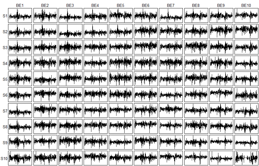
We apply our model (4) to fit the standardized matrix time series $\{{\mathbf{Y}}_{t}\}_{t=1}^{336}$ using the refined estimation method with PCA-based $\xi_{t}$ ; leading to $\hat{d}\equiv 1$ with $K=3,5$ or 7. See (30). In the sequel, we only present the results with $K=5$ . The results based on $K\in\{3,7\}$ are similar and thus omitted here. Based on (34), we obtain $\widehat{{\mathbf{A}}}=(0.44,0.34,0.32,0.32,0.29,0.25,0.30,0.30,0.33,0.23)^{\scriptscriptstyle\top}$ and $\widehat{{\mathbf{B}}}=(0.20,0.26,0.27,0.29,0.35,0.33,0.34,0.31,0.37,0.39)^{\scriptscriptstyle\top}$ . Following the arguments above Proposition 1 in Section 3.1, we can recover the latent time series $\{\hat{x}_{t,1}\}_{t=1}^{336}$ . Figure 4 displays the plots of time series $\{\hat{x}_{t,1}\}_{t=1}^{336}$ and its ACF, which shows that the autocorrelations of $\{\hat{x}_{t,1}\}_{t=1}^{336}$ is significant at the first lag that is consistent to the ACF patterns of ${\mathbf{Y}}_{t}$ . The Akaike information criterion (AIC) suggests to fit $\{\hat{x}_{t,1}\}_{t=1}^{336}$ by an AR(1) model. Hence, to model this $10\times 10$ matrix time series ${\mathbf{Y}}_{t}$ , our method essentially only needs to estimate one parameter in an AR(1) model. We also consider to fit the matrix time series ${\mathbf{Y}}_{t}$ by following methods:

•

(UniARMA) For each of 100 component time series $\{y_{i,j,t}\}_{t=1}^{336}$ , we fit an ARMA model specified by the AIC; leading to the estimation for 135 coefficient parameters in the total 100 models.
•

(SVAR) Fit a sparse VAR( $\ell$ ) model to $\{{\rm vec}({\mathbf{Y}}_{t})\}_{t=1}^{336}$ using the R-function sparseVAR in the R-package bigtime with the standard lasso penalization and the optimal sparsity parameter selected by the time series cross validation procedure. The program selects $\ell=27$ automatically based on the time series length, and there are 270000 parameters to be estimated.
•

(MAR) Fit $\{{\mathbf{Y}}_{t}\}_{t=1}^{336}$ by the matrix-AR(1) of Chen et al. 2021, which involves 200 parameters.
•

(TS-PCA) Apply the principle component analysis for time series suggested in Chang et al. 2018 to the 100-dimensional time series $\{{\rm vec}({\mathbf{Y}}_{t})\}_{t=1}^{336}$ using the R-package HDTSA, leading to 98 univariate time series and one two-dimensional time series. For the obtained univariate time series, we fit it by an ARMA model with the order determined by the AIC. For the obtained two-dimensional time series, we fit it by an VAR model with the order determined by the AIC. There are in total 93 parameters in the models.
•

(FAC) Apply the factor model of Wang et al. 2019 to matrix time series $\{{\mathbf{Y}}_{t}\}_{t=1}^{336}$ with the pre-determined parameter $h_{0}=1$ as suggested in the real data analysis part of their paper. Based on their method, we find there is only one factor. We fit the latent factor series by an AR(1) model specified by the AIC which only needs to estimate one parameter.

While UniARMA, SVAR and MAR model ${\mathbf{Y}}_{t}$ or $\mathrm{vec}({\mathbf{Y}}_{t})$ directly, our proposed method, TS-PCA and FAC seek dimension reduction first and then model the resulting low-dimensional time series. Both RMSE and MAE, defined as below, of the fitted models are listed in Table 2:

\mathrm{RMSE}=\bigg\{\frac{1}{33600}\sum_{t=1}^{336}\sum_{i=1}^{10}\sum_{j=1}^{10}(\hat{y}_{i,j,t}-y_{i,j,t})^{2}\bigg\}^{1/2}\,,~~~\mathrm{MAE}=\frac{1}{33600}\sum_{t=1}^{336}\sum_{i=1}^{10}\sum_{j=1}^{10}|\hat{y}_{i,j,t}-y_{i,j,t}|\,.

Among the three dimension-reduction methods, our proposed method has the smallest RMSE and MAE, while MAR achieves the overall minimum RMSE and MAE.

Table 2: Fitting errors for the monthly data from year 1990 to 2017. The computational time is conducted on the Windows platform with Intel(R) Core(TM) i7-8550U CPU at 1.99 GHz.

	Proposed	TS-PCA	FAC	UniARMA	SVAR	MAR
RMSE	0.9913	0.9935	0.9923	0.9895	0.9985	0.9613
MAE	0.7432	0.7456	0.7436	0.7417	0.7444	0.7235
$\#$ Parameters	1	93	1	135	270000	200
time (seconds)	0.3172	6.4618	0.6596	6.7335	1689.1860	1.8470

We also evaluate the post-sample forecasting performance of these methods by performing the one-step and two-step ahead rolling forecasts for the 24 monthly readings in the last two years (i.e. 2016 and 2017). For each $s=1,\ldots,24$ , we use our proposed method and the other five methods to fit $\{{\mathbf{Y}}_{t}\}_{t=s}^{311+s}$ and then obtain the one-step forecast of ${\mathbf{Y}}_{312+s}$ denoted by $\widehat{{\mathbf{Y}}}_{312+s}=\{\hat{y}_{i,j,312+s}^{(s)}\}_{10\times 10}$ . For the two-step ahead forecast, we fit $\{{\mathbf{Y}}_{t}\}_{t=s}^{310+s}$ by the six methods, and the two-step ahead forecast $\widehat{{\mathbf{Y}}}_{312+s}$ can be obtained by plug-in the one-step forecast into the models. For our proposed method, TS-PCA and FAC, if the dimension of the obtained latent time series is larger than $1$ we fit it by a VAR model with the order determined by the AIC, otherwise we fit it by an ARMA model with the order determined by the AIC. The post-sample forecasting performance is evaluated by the rRMSE and rMAE defined as

	$\displaystyle{\rm rRMSE}=$	$\displaystyle~\bigg[\frac{1}{2400}\sum_{s=1}^{24}\sum_{i=1}^{10}\sum_{j=1}^{10}\{\hat{y}_{i,j,312+s}^{(s)}-y_{i,j,312+s}\}^{2}\bigg]^{1/2}\,,$
	$\displaystyle{\rm rMAE}=$	$\displaystyle~\frac{1}{2400}\sum_{s=1}^{24}\sum_{i=1}^{10}\sum_{j=1}^{10}\big\|\hat{y}_{i,j,312+s}^{(s)}-y_{i,j,312+s}\big\|\,.$

Table 3 summarizes the post-sample forecasting rRMSE and rMAE. The newly proposed method, in spite of its simplicity, exhibits the promising post-sample forecasting performance, as its rRMSE and rMAE are the smallest in one-step ahead forecasting among all the methods concerned, and are the 2nd smallest in the two-step ahead forecast for which only TS-PCA has smaller rRMSE and rMAE.

Table 3: One-step and two-step ahead forecasting errors for the monthly readings in the last two years 2016 and 2017.

	Proposed	TS-PCA	FAC	UniARMA	SVAR	MAR
	one-step ahead forecast
rRMSE	0.7678	0.7802	0.7701	0.7724	0.7690	0.8067
rMAE	0.5609	0.5696	0.5649	0.5652	0.5614	0.5948
	two-step ahead forecast
rRMSE	0.7668	0.7526	0.7683	0.7707	0.7693	0.7728
rMAE	0.5590	0.5512	0.5610	0.5638	0.5616	0.5627

Acknowledgements

We thank the editor, the associate editor and two referees for their constructive comments. Chang, He and Yang were supported in part by the National Natural Science Foundation of China (grant nos. 71991472, 72125008, 11871401 and 11701466). Yao was supported in part by the U.K. Engineering and Physical Sciences Research Council. Chang was also supported by the Center of Statistical Research at Southwestern University of Finance and Economics.

References

(1)
Anandkumar et al. (2014) Anandkumar, A., Ge, R. and Janzamin, M. (2014). Guaranteed non-orthogonal tensor decomposition via alternating rank-1 updates. arXiv:1402.5180.
Bickel and Levina (2008) Bickel, P. J. and Levina, E. (2008). Covariance regularization by thresholding. The Annals of Statistics, 36, 2577–2604.
Chang et al. (2021) Chang, J., Chen, X. and Wu, M. (2021). Central limit theorems for high dimentional dependent data. arXiv:2104.12929.
Chang et al. (2015) Chang, J., Guo, B. and Yao, Q. (2015). High dimensional stochastic regression with latent factors, endogeneity and nonlinearity. Journal of Econometrics, 189, 297–312.
Chang et al. (2018) Chang, J., Guo, B. and Yao, Q. (2018). Principal component analysis for second-order stationary vector time series. The Annals of Statistics, 46, 2094–2124.
Chang et al. (2022) Chang, J., Hu, Q., Liu, C. and Tang, C. Y. (2022). Optimal covariance matrix estimation for high-dimensional noise in high-frequency data. Journal of Econometrics, in press.
Chang et al. (2013) Chang, J., Tang, C. Y. and Wu, Y. (2013). Marginal empirical likelihood and sure independence feature screening. The Annals of Statistics, 41, 2123–2148.
Chen and Chen (2019) Chen, E. Y. and Chen, R. (2019). Modeling dynamic transport network with matrix factor models: with an application to international trade flow. arXiv:1901.00769.
Chen et al. (2020) Chen, E. Y., Tsay, R. S. and Chen, R. (2020). Constrained factor models for high-dimensional matrix-variate time series. Journal of the American Statistical Association, 115, 775–793.
Chen et al. (2021) Chen, R., Xiao, H. and Yang, D. (2021). Autoregressive models for matrix-valued time series. Journal of Econometrics, 222, 539–560.
Colombo and Vlassis (2016) Colombo, N. and Vlassis, N. (2016). Tensor decomposition via joint matrix schur decomposition. International Conference on Machine Learning, PMLR 48, 2820–2828.
Domanov and De Lathauwer (2014) Domanov, I. and De Lathauwer, L. (2014). Canonical polyadic decomposition of third-order tensors: reduction to generalized eigenvalue decomposition. SIAM Journal of Matrix Analysis and Applications, 35, 636–660.
Golub and Van Loan (2013) Golub, G. H. and Van Loan, C. F. (2013). Matrix Computations (4th Edition). Johns Hopkins University Press, Baltimore.
Han et al. (2021a) Han, Y., Chen, R., Zhang, C.-H. and Yao, Q. (2021a). Simultaneous decorrelation of matrix time series. arXiv:2103.09411.
Han and Zhang (2021) Han, Y. and Zhang, C.-H. (2021). Tensor principal component analysis in high dimensional CP models. arXiv:2108.04428.
Han et al. (2021b) Han, Y., Zhang, C.-H. and Chen, R. (2021b). CP factor model for dynamic tensors. arXiv:2110.15517.
Kolda and Bader (2009) Kolda, T. G. and Bader, B. W. (2009). Tensor decompositions and applications. SIAM Review, 51, 455–500.
Lam and Yao (2012) Lam, C. and Yao, Q. (2012). Factor modelling for high-dimensional time series: inference for the number of factors. The Annals of Statistics, 40, 694–726.
Liu et at. (2014) Liu, Y., Shang, F., Fan, W., Cheng, J. and Cheng, H. (2014). Generalized higher-order orthogonal iteration for tensor decomposition and completion. In Advances in Neural Information Processing Systems, 1763–1771.
Sanchez and Kowalski (1990) Sanchez, E. and Kowalski, B. R. (1990). Tensorial resolution: a direct trilinear decomposition. Journal of Chemometrics, 4, 29–45.
Sharan and Valiant (2017) Sharan, V. and Valiant, G. (2017). Orthogonalized als: A theoretically principled tensor decomposition algorithm for practical use. International Conference on Machine Learning, PMLR 70, 3095–3104.
Sun at al. (2017) Sun, W. W., Lu, J., Liu, H. and Cheng, G. (2017). Provable sparse tensor decomposition. Journal of the Royal Statistical Society B, 79, 899–916.
Wang et al. (2019) Wang, D., Liu, X. and Chen, R. (2019). Factor models for matrix-valued high-dimensional time series. Journal of Econometrics, 208, 231–248.
Wang and Song (2017) Wang, M. and Song, Y. (2017). Tensor decompositions via two-mode higher-order svd (hosvd). International Conference on Artificial Intelligence and Statistics, PMLR 54, 614–622.
Zhang and Xia (2018) Zhang, A. and Xia, D. (2018). Tensor svd: Statistical and computational limits. IEEE Transactions on Information Theory, 64, 7311–7338.

Supplementary Material for “Modelling Matrix Time Series via a Tensor CP-Decomposition” by Jinyuan Chang, Jing He, Lin Yang and Qiwei Yao

Throughout the supplementary material, we use $C\in(0,\infty)$ to denote a generic finite constant that does not depend on $(n,p,q,d)$ , and may be different in different uses. For two sequences of positive numbers $\{a_{n}\}$ and $\{b_{n}\}$ , we write $a_{n}\lesssim b_{n}$ or $b_{n}\gtrsim a_{n}$ if $\limsup_{n\rightarrow\infty}a_{n}/b_{n}\leq c_{0}$ for some constant $c_{0}>0$ .

Appendix A Proof of Proposition 1

Recall $\widehat{{\mathbf{K}}}_{2,q}\hat{{\mathbf{b}}}^{\ell}=\lambda_{*}\widetilde{{\mathbf{K}}}_{1,q}\hat{{\mathbf{b}}}^{\ell}$ . Then $\widehat{{\mathbf{K}}}_{2,q}\overline{\hat{{\mathbf{b}}}^{\ell}}=\overline{\lambda_{*}}\widetilde{{\mathbf{K}}}_{1,q}\overline{\hat{{\mathbf{b}}}^{\ell}}$ , where $\overline{\hat{{\mathbf{b}}}^{\ell}}$ is the complex conjugate of $\hat{{\mathbf{b}}}^{\ell}$ . Hence, $\overline{\lambda_{*}}$ and $\overline{\hat{{\mathbf{b}}}^{\ell}}$ are, respectively, the eigenvalue and the associated eigenvector of the generalized eigenequation $\widehat{{\mathbf{K}}}_{2,q}{\mathbf{b}}=\lambda\widetilde{{\mathbf{K}}}_{1,q}{\mathbf{b}}$ . Since the eigenvalues of $\widehat{{\mathbf{K}}}_{2,q}{\mathbf{b}}=\lambda\widetilde{{\mathbf{K}}}_{1,q}{\mathbf{b}}$ are distinct, there exists $\tilde{\ell}\in[\hat{d}]$ and a constant $\kappa\in\{-1,1\}$ such that $\overline{\hat{{\mathbf{b}}}^{\ell}}=\kappa\hat{{\mathbf{b}}}^{\tilde{\ell}}$ . By (19), we have

\hat{{\mathbf{a}}}_{\tilde{\ell}}=\frac{\widehat{\mathbf{\Sigma}}_{1}\hat{{\mathbf{b}}}^{\tilde{\ell}}}{|\widehat{\mathbf{\Sigma}}_{1}\hat{{\mathbf{b}}}^{\tilde{\ell}}|_{2}}=\frac{\kappa\widehat{\mathbf{\Sigma}}_{1}\overline{\hat{{\mathbf{b}}}^{\ell}}}{|\widehat{\mathbf{\Sigma}}_{1}\overline{\hat{{\mathbf{b}}}^{\ell}}|_{2}}=\kappa\overline{\hat{{\mathbf{a}}}_{\ell}}\,,

(S.1)

where $\overline{\hat{{\mathbf{a}}}_{\ell}}$ is the complex conjugate of $\hat{{\mathbf{a}}}_{\ell}$ .

Recall $\widehat{{\mathbf{A}}}^{+}=(\hat{{\mathbf{a}}}^{1},\ldots,\hat{{\mathbf{a}}}^{\hat{d}})^{\scriptscriptstyle\top}$ is the Moore-Penrose inverse of $\widehat{{\mathbf{A}}}=(\hat{{\mathbf{a}}}_{1},\ldots,\hat{{\mathbf{a}}}_{\hat{d}})$ . To show $\hat{{\mathbf{b}}}_{\tilde{\ell}}=\kappa\overline{\hat{{\mathbf{b}}}_{\ell}}$ , by (20), we only need to show $\hat{{\mathbf{a}}}^{\tilde{\ell}}=\kappa\overline{\hat{{\mathbf{a}}}^{\ell}}$ . Assume the generalized eigenequation $\widehat{{\mathbf{K}}}_{2,q}{\mathbf{b}}=\lambda\widetilde{{\mathbf{K}}}_{1,q}{\mathbf{b}}$ has $s$ real eigenvalues. Then there are $\hat{d}-s$ complex eigenvalues. Since the complex eigenvalues always occur in complex conjugate pairs, $\hat{d}-s$ is an even integer. Write $\hat{d}-s=2m$ . Let $\lambda_{1},\overline{\lambda_{1}},\ldots,\lambda_{m},\overline{\lambda_{m}}$ be the $\hat{d}-s$ complex eigenvalues of the generalized eigenequation $\widehat{{\mathbf{K}}}_{2,q}{\mathbf{b}}=\lambda\widetilde{{\mathbf{K}}}_{1,q}{\mathbf{b}}$ . For each $j\in[m]$ , there exist $\ell_{j},\tilde{\ell}_{j}\in[\hat{d}]$ such that the eigenvectors associated with $\lambda_{j}$ and $\overline{\lambda_{j}}$ are, respectively, $\hat{{\mathbf{b}}}^{\ell_{j}}$ and $\hat{{\mathbf{b}}}^{\tilde{\ell}_{j}}$ . Then there exists $(\kappa_{1},\ldots,\kappa_{m})\in\{-1,1\}^{m}$ such that $\hat{{\mathbf{b}}}^{\tilde{\ell}_{j}}=\kappa_{j}\overline{\hat{{\mathbf{b}}}^{\ell_{j}}}$ for each $j\in[m]$ . Same as (S.1), we have $\hat{{\mathbf{a}}}_{\tilde{\ell}_{j}}=\kappa_{j}\overline{\hat{{\mathbf{a}}}_{\ell_{j}}}$ for each $j\in[m]$ . Write $\boldsymbol{\varpi}_{j}={\rm Re}(\hat{{\mathbf{a}}}_{\ell_{j}})$ and $\boldsymbol{\varsigma}_{j}={\rm Im}(\hat{{\mathbf{a}}}_{\ell_{j}})$ for each $j\in[m]$ . Then $\hat{{\mathbf{a}}}_{\tilde{\ell}_{j}}=\kappa_{j}\boldsymbol{\varpi}_{j}-{\rm i}\kappa_{j}\boldsymbol{\varsigma}_{j}$ for each $j\in[m]$ , where ${\rm i}=\sqrt{-1}$ . Let $\{j_{1},\ldots,j_{s}\}=[\hat{d}]\setminus\{\ell_{1},\tilde{\ell}_{1},\ldots,\ell_{m},\tilde{\ell}_{m}\}$ . For each $r\in[s]$ , $\hat{{\mathbf{b}}}^{j_{r}}$ are the eigenvector of the generalized eigenequation $\widehat{{\mathbf{K}}}_{2,q}{\mathbf{b}}=\lambda\widetilde{{\mathbf{K}}}_{1,q}{\mathbf{b}}$ associated with the real eigenvalue $\tilde{\lambda}_{r}$ . Write $\hat{{\mathbf{b}}}^{j_{r}}={\rm Re}(\hat{{\mathbf{b}}}^{j_{r}})+{\rm i}\,{\rm Im}(\hat{{\mathbf{b}}}^{j_{r}})$ . Since $\widetilde{{\mathbf{K}}}_{1,q}$ and $\widehat{{\mathbf{K}}}_{2,q}$ are two real matrices, then ${\rm Re}(\hat{{\mathbf{b}}}^{j_{r}})$ and ${\rm Im}(\hat{{\mathbf{b}}}^{j_{r}})$ are both the eigenvectors of the generalized eigenequation $\widehat{{\mathbf{K}}}_{2,q}{\mathbf{b}}=\lambda\widetilde{{\mathbf{K}}}_{1,q}{\mathbf{b}}$ associated with the real eigenvalue $\tilde{\lambda}_{r}$ . Recall the eigenvalues of the generalized eigenequation $\widehat{{\mathbf{K}}}_{2,q}{\mathbf{b}}=\lambda\widetilde{{\mathbf{K}}}_{1,q}{\mathbf{b}}$ are distinct. There exists a constant $c_{r}\in\mathbb{R}$ such that ${\rm Im}(\hat{{\mathbf{b}}}^{j_{r}})=c_{r}{\rm Re}(\hat{{\mathbf{b}}}^{j_{r}})$ . Thus, any eigenvector of the generalized eigenequation $\widehat{{\mathbf{K}}}_{2,q}{\mathbf{b}}=\lambda\widetilde{{\mathbf{K}}}_{1,q}{\mathbf{b}}$ associated with the real eigenvalue $\tilde{\lambda}_{r}$ can be formulated as $\tilde{c}_{r}{\rm Re}(\hat{{\mathbf{b}}}^{j_{r}})$ for some $\tilde{c}_{r}\in\mathbb{C}$ . Without loss of generality, we can assume $\hat{{\mathbf{b}}}^{j_{1}},\ldots,\hat{{\mathbf{b}}}^{j_{s}}$ are all real vectors. Notice that there exists a $\hat{d}\times\hat{d}$ real matrix ${\mathbf{F}}$ such that

	$\displaystyle\widehat{{\mathbf{A}}}{\mathbf{F}}=$	$\displaystyle\,(\hat{{\mathbf{a}}}_{\ell_{1}},\hat{{\mathbf{a}}}_{\tilde{\ell}_{1}},\ldots,\hat{{\mathbf{a}}}_{\ell_{m}},\hat{{\mathbf{a}}}_{\tilde{\ell}_{m}},\hat{{\mathbf{a}}}_{j_{1}},\ldots,\hat{{\mathbf{a}}}_{j_{s}})$
	$\displaystyle=$	$\displaystyle\,\underbrace{(\boldsymbol{\varpi}_{1},\boldsymbol{\varsigma}_{1},\ldots,\boldsymbol{\varpi}_{m},\boldsymbol{\varsigma}_{m},\hat{{\mathbf{a}}}_{j_{1}},\ldots,\hat{{\mathbf{a}}}_{j_{s}})}_{{\mathbf{S}}}{\rm diag}({\mathbf{K}}_{1},\ldots,{\mathbf{K}}_{m},{\mathbf{I}}_{s})\,,$		(S.2)

where

{\mathbf{K}}_{j}=\left(\begin{array}[]{cc}1&1\\ \rm{i}&-\rm{i}\\ \end{array}\right)\left(\begin{array}[]{cc}1&0\\ 0&\kappa_{j}\\ \end{array}\right)\,,~~~j\in[m]\,.

The matrix ${\mathbf{F}}$ essentially exchanges the columns of $\widehat{{\mathbf{A}}}$ which is invertible. Without loss of generality, we assume $(\ell,\tilde{\ell})=(\ell_{1},\tilde{\ell}_{1})$ . Then $\kappa_{1}=\kappa$ . Since $\widehat{{\mathbf{A}}}$ has full column rank, $\widehat{{\mathbf{A}}}^{+}=(\widehat{{\mathbf{A}}}^{\scriptscriptstyle\mathrm{H}}\widehat{{\mathbf{A}}})^{-1}\widehat{{\mathbf{A}}}^{\scriptscriptstyle\mathrm{H}}$ , where ^H denotes the conjugate transpose. Notice that ${\mathbf{S}}$ is a real matrix. By (S.2), it holds that

\widehat{{\mathbf{A}}}^{+}={\mathbf{F}}{\rm diag}({\mathbf{K}}_{1}^{-1},\ldots,{\mathbf{K}}_{m}^{-1},{\mathbf{I}}_{s})({\mathbf{S}}^{\scriptscriptstyle\top}{\mathbf{S}})^{-1}{\mathbf{S}}^{\scriptscriptstyle\top}\,.

Since the first two rows of ${\mathbf{F}}^{\scriptscriptstyle\top}\widehat{{\mathbf{A}}}^{+}$ are $(\hat{{\mathbf{a}}}^{\ell})^{\scriptscriptstyle\top}$ and $(\hat{{\mathbf{a}}}^{\tilde{\ell}})^{\scriptscriptstyle\top}$ , due to the fact ${\mathbf{F}}^{\scriptscriptstyle\top}{\mathbf{F}}={\mathbf{I}}_{\hat{d}}$ , we have $(\hat{{\mathbf{a}}}^{\ell},\hat{{\mathbf{a}}}^{\tilde{\ell}})^{\scriptscriptstyle\top}=({\mathbf{K}}_{1}^{-1},{\mathbf{0}})({\mathbf{S}}^{\scriptscriptstyle\top}{\mathbf{S}})^{-1}{\mathbf{S}}^{\scriptscriptstyle\top}$ , which implies

\hat{{\mathbf{a}}}^{\ell}=\frac{1}{2}{\mathbf{S}}({\mathbf{S}}^{\scriptscriptstyle\top}{\mathbf{S}})^{-1}(1,-{\rm i},{\mathbf{0}})^{\scriptscriptstyle\top}~~\textrm{and}~~\hat{{\mathbf{a}}}^{\tilde{\ell}}=\frac{1}{2}{\mathbf{S}}({\mathbf{S}}^{\scriptscriptstyle\top}{\mathbf{S}})^{-1}(\kappa,{\rm i}\kappa,{\mathbf{0}})^{\scriptscriptstyle\top}\,.

Hence, $\hat{{\mathbf{a}}}^{\tilde{\ell}}=\kappa\overline{\hat{{\mathbf{a}}}^{\ell}}$ .

Recall $(\hat{x}_{t,1},\ldots,\hat{x}_{t,\hat{d}})^{\scriptscriptstyle\top}=\widehat{\mathbf{H}}^{+}\mathrm{vec}({\mathbf{Y}}_{t})$ with $\widehat{{\mathbf{H}}}=(\hat{{\mathbf{b}}}_{1}\otimes\hat{{\mathbf{a}}}_{1},\ldots,\hat{{\mathbf{b}}}_{\hat{d}}\otimes\hat{{\mathbf{a}}}_{\hat{d}})$ . Since $\hat{{\mathbf{b}}}_{\tilde{\ell}}\otimes\hat{{\mathbf{a}}}_{\tilde{\ell}}$ is the complex conjugate of $\hat{{\mathbf{b}}}_{{\ell}}\otimes\hat{{\mathbf{a}}}_{{\ell}}$ , following the same arguments stated above, we know the $\tilde{\ell}$ -th row of $\widehat{\mathbf{H}}^{+}$ is the complex conjugate of the ${\ell}$ -th row of $\widehat{\mathbf{H}}^{+}$ , which yields that $\hat{x}_{t,\tilde{\ell}}=\overline{\hat{x}_{t,{\ell}}}$ . $\hfill\Box$

Appendix B Proofs of Theorem 1 and Proposition 3

Recall $\Pi_{1,n}=(s_{1}s_{2})^{1/2}\{{n}^{-1}{\log(pq)}\}^{(1-\iota)/2}$ . To construct Theorem 1 and Proposition 3, we need the following lemma whose proof is given in Section D.1.

Lemma 1.

Under Conditions 3 and 4, if the threshold level $\delta_{1}=C_{*}\{n^{-1}\log(pq)\}^{1/2}$ for some sufficiently large constant $C_{*}>0$ , we have $\|\widehat{{\mathbf{M}}}_{1}-{\mathbf{M}}_{1}\|_{2}=O_{\rm p}(\Pi_{1,n})=\|\widehat{{\mathbf{M}}}_{2}-{\mathbf{M}}_{2}\|_{2}$ , provided that $\Pi_{1,n}=o(1)$ and $\log(pq)=o(n^{c})$ for some constant $c\in(0,1)$ depending only on $r_{1}$ and $r_{2}$ specified in Condition 4.

B.1 Proof of Theorem 1

Denote by $\hat{\lambda}_{1}\geq\cdots\geq\hat{\lambda}_{p}$ and ${\lambda}_{1}\geq\cdots\geq\lambda_{p}$ , respectively, the eigenvalues of $\widehat{{\mathbf{M}}}_{1}$ and ${\mathbf{M}}_{1}$ . By Lemma 1, $\max_{i\in[p]}|\hat{\lambda}_{i}-\lambda_{i}|\leq\|\widehat{{\mathbf{M}}}_{1}-{\mathbf{M}}_{1}\|_{2}=o_{\rm p}(c_{n})$ for some $c_{n}=o(1)$ satisfying $\Pi_{1,n}=o(c_{n})$ . By Condition 2, we know $\lambda_{d}\geq C$ , and $\lambda_{d+1}=\cdots=\lambda_{p}=0$ . Hence, for any $j<d$ , $(\hat{\lambda}_{j+1}+c_{n})/(\hat{\lambda}_{j}+c_{n})\stackrel{{\scriptstyle\mathbb{P}}}{{\rightarrow}}\lambda_{j+1}/\lambda_{j}>0$ . For any $j>d$ , note that $|\hat{\lambda}_{j}|=o_{\rm p}(c_{n})$ , then $(\hat{\lambda}_{j+1}+c_{n})/(\hat{\lambda}_{j}+c_{n})\stackrel{{\scriptstyle\mathbb{P}}}{{\rightarrow}}1$ . On the other hand, $(\hat{\lambda}_{d+1}+c_{n})/(\hat{\lambda}_{d}+c_{n})\stackrel{{\scriptstyle\mathbb{P}}}{{\rightarrow}}0$ , which implies $(\hat{\lambda}_{d+1}+c_{n})/(\hat{\lambda}_{d}+c_{n})=\min_{j\in[R]}(\hat{\lambda}_{j+1}+c_{n})/(\hat{\lambda}_{j}+c_{n})$ with probability approaching one. This indicates that $\mathbb{P}(\hat{d}=d)\rightarrow 1$ as $n\rightarrow\infty$ . $\hfill\Box$

B.2 Proof of Proposition 3

Denote by $\lambda_{1,1}\geq\cdots\geq\lambda_{1,p}$ and ${\lambda}_{2,1}\geq\cdots\geq\lambda_{2,q}$ , respectively, the eigenvalues of ${\mathbf{M}}_{1}$ and ${\mathbf{M}}_{2}$ . It follows from Condition 2 that $\lambda_{1,1}\geq\cdots\geq\lambda_{1,d}>0=\lambda_{1,d+1}=\cdots=\lambda_{1,p}$ and $\lambda_{2,1}\geq\cdots\geq\lambda_{2,d}>0=\lambda_{2,d+1}=\cdots=\lambda_{2,q}$ . Notice that $\lambda_{1,d}$ and $\lambda_{2,d}$ are uniformly bounded away from zero. Lemma 1 of Chang et al. 2018 implies that $\|\widehat{{\mathbf{P}}}{\mathbf{E}}_{1}-{\mathbf{P}}\|_{2}\leq C\|\widehat{{\mathbf{M}}}_{1}-{\mathbf{M}}_{1}\|_{2}$ and $\|\widehat{{\mathbf{Q}}}{\mathbf{E}}_{2}-{\mathbf{Q}}\|_{2}\leq C\|\widehat{{\mathbf{M}}}_{2}-{\mathbf{M}}_{2}\|_{2}$ , where ${\mathbf{E}}_{1}$ and ${\mathbf{E}}_{2}$ are two orthogonal matrices. Together with Lemma 1, we complete the proof of Proposition 3. $\hfill\Box$

Appendix C Proof of Theorem 2

Recall $\Pi_{1,n}=(s_{1}s_{2})^{1/2}\{{n}^{-1}{\log(pq)}\}^{(1-\iota)/2}$ and $\Pi_{2,n}=(s_{3}s_{4})^{1/2}\{{n}^{-1}{\log(pq)}\}^{(1-\iota)/2}$ . Write $\Pi_{n}=\Pi_{1,n}+\Pi_{2,n}$ . For $\widehat{\mathbf{\Sigma}}_{{\mathbf{Z}},\eta}(k)$ defined as (32), we write

		$\displaystyle\widehat{{\mathbf{S}}}_{1}=\widehat{\mathbf{\Sigma}}_{{\mathbf{Z}},\eta}(1)^{\scriptscriptstyle\top}\widehat{\mathbf{\Sigma}}_{{\mathbf{Z}},\eta}(1)\,,~~~\widehat{{\mathbf{S}}}_{2}=\widehat{\mathbf{\Sigma}}_{{\mathbf{Z}},\eta}(1)^{\scriptscriptstyle\top}\widehat{\mathbf{\Sigma}}_{{\mathbf{Z}},\eta}(2)\,,$
		$\displaystyle\widehat{{\mathbf{S}}}_{1}^{}=\widehat{\mathbf{\Sigma}}_{{\mathbf{Z}},\eta}(1)\widehat{\mathbf{\Sigma}}_{{\mathbf{Z}},\eta}(1)^{\scriptscriptstyle\top}\,,~~~\widehat{{\mathbf{S}}}_{2}^{}=\widehat{\mathbf{\Sigma}}_{{\mathbf{Z}},\eta}(1)\widehat{\mathbf{\Sigma}}_{{\mathbf{Z}},\eta}(2)^{\scriptscriptstyle\top}\,.$

Recall $\widetilde{{\mathbf{S}}}_{1}={\mathbf{\Sigma}}_{{\mathbf{Z}},\tilde{\eta}}(1)^{\scriptscriptstyle\top}{\mathbf{\Sigma}}_{{\mathbf{Z}},\tilde{\eta}}(1)$ , $\widetilde{{\mathbf{S}}}_{2}={\mathbf{\Sigma}}_{{\mathbf{Z}},\tilde{\eta}}(1)^{\scriptscriptstyle\top}{\mathbf{\Sigma}}_{{\mathbf{Z}},\tilde{\eta}}(2)$ , $\widetilde{{\mathbf{S}}}_{1}^{*}={\mathbf{\Sigma}}_{{\mathbf{Z}},\tilde{\eta}}(1){\mathbf{\Sigma}}_{{\mathbf{Z}},\tilde{\eta}}(1)^{\scriptscriptstyle\top}$ and $\widetilde{{\mathbf{S}}}_{2}^{*}={\mathbf{\Sigma}}_{{\mathbf{Z}},\tilde{\eta}}(1){\mathbf{\Sigma}}_{{\mathbf{Z}},\tilde{\eta}}(2)^{\scriptscriptstyle\top}$ . To construct Theorem 2, we need the following lemmas. The proofs of Lemmas 2 and 3 are given in Sections D.2 and D.3, respectively. Lemma 4 is Corollary 7.2.6 of Golub and Van Loan 2013.

Lemma 2.

Under Conditions 1–4, and 6, if the threshold levels $\delta_{1}=C_{*}\{n^{-1}\log(pq)\}^{1/2}$ and $\delta_{2}=C_{**}\{n^{-1}\log(pq)\}^{1/2}$ for some sufficiently large constants $C_{*}>0$ and $C_{**}>0$ , we have $\max_{k\in\{1,2\}}\|{\mathbf{E}}_{1}^{\scriptscriptstyle\top}\widehat{\mathbf{\Sigma}}_{{\mathbf{Z}},\eta}(k){\mathbf{E}}_{2}-{\mathbf{\Sigma}}_{{\mathbf{Z}},\tilde{\eta}}(k)\|_{2}=O_{\rm p}(\Pi_{n})$ for $({\mathbf{E}}_{1},{\mathbf{E}}_{2})$ specified in Proposition 3, provided that $\Pi_{n}=o(1)$ and $\log(pq)=o(n^{c})$ for some constant $c\in(0,1)$ depending only on $r_{1}$ and $r_{2}$ specified in Condition 4.

Lemma 3.

Under conditions of Lemma 2, we have $\|{\mathbf{E}}_{2}^{\scriptscriptstyle\top}\widehat{{\mathbf{S}}}_{1}{\mathbf{E}}_{2}-\widetilde{\mathbf{S}}_{1}\|_{2}=O_{\rm p}(\Pi_{n})=\|{\mathbf{E}}_{2}^{\scriptscriptstyle\top}\widehat{{\mathbf{S}}}_{2}{\mathbf{E}}_{2}-\widetilde{\mathbf{S}}_{2}\|_{2}$ and $\|{\mathbf{E}}_{1}^{\scriptscriptstyle\top}\widehat{{\mathbf{S}}}_{1}^{*}{\mathbf{E}}_{1}-\widetilde{\mathbf{S}}_{1}^{*}\|_{2}=O_{\rm p}(\Pi_{n})=\|{\mathbf{E}}_{1}^{\scriptscriptstyle\top}\widehat{{\mathbf{S}}}_{2}^{*}{\mathbf{E}}_{1}-\widetilde{\mathbf{S}}_{2}^{*}\|_{2}$ for $({\mathbf{E}}_{1},{\mathbf{E}}_{2})$ specified in Proposition 3.

Lemma 4.

Suppose ${\mathbf{W}},\boldsymbol{\Delta}\in\mathbb{C}^{d\times d}$ and that ${\mathbf{R}}=({\mathbf{r}}_{1},{\mathbf{R}}_{2})\in\mathbb{C}^{d\times d}$ is unitary with ${\mathbf{r}}_{1}\in\mathbb{C}^{d}$ . Assume

\displaystyle{\mathbf{R}}^{\scriptscriptstyle\mathrm{H}}{\mathbf{W}}{\mathbf{R}}=\left(\begin{array}[]{cc}\lambda&{\mathbf{v}}^{\scriptscriptstyle\mathrm{H}}\\ {\mathbf{0}}&{\mathbf{D}}_{22}\\ \end{array}\right)~~\textrm{and}~~{\mathbf{R}}^{\scriptscriptstyle\mathrm{H}}\boldsymbol{\Delta}{\mathbf{R}}=\left(\begin{array}[]{cc}\epsilon&\boldsymbol{\gamma}^{\scriptscriptstyle\mathrm{H}}\\ \boldsymbol{\delta}&\boldsymbol{\Delta}_{22}\\ \end{array}\right),

where ^H denotes the conjugate transpose. Let $\theta$ be the smallest singular value of ${\mathbf{D}}_{22}-\lambda{\mathbf{I}}_{d-1}$ , and denote by $\|\cdot\|_{\rm F}$ the Frobenius norm of $\cdot$ . If $\theta>0$ and $5\|\boldsymbol{\Delta}\|_{\rm F}(1+5\theta^{-1}|{\mathbf{v}}|_{2})\leq\theta$ , then there exists ${\mathbf{u}}\in\mathbb{C}^{d-1}$ with $|{\mathbf{u}}|_{2}\leq 4\theta^{-1}|\boldsymbol{\delta}|_{2}$ such that $\tilde{{\mathbf{r}}}_{1}=({\mathbf{r}}_{1}+{\mathbf{R}}_{2}{\mathbf{u}})/\sqrt{1+{\mathbf{u}}^{\scriptscriptstyle\mathrm{H}}{\mathbf{u}}}$ is a unit $\ell^{2}$ -norm eigenvector for ${\mathbf{W}}+\boldsymbol{\Delta}$ .

Now we begin to prove Theorem 2. Let $\{\hat{\boldsymbol{\beta}}_{{\mathbf{v}},1},\ldots,\hat{\boldsymbol{\beta}}_{{\mathbf{v}},d}\}$ and $\{\boldsymbol{\beta}_{{\mathbf{v}},1},\ldots,\boldsymbol{\beta}_{{\mathbf{v}},d}\}$ be, respectively, the eigenvectors of $\widehat{{\mathbf{S}}}_{1}^{-1}\widehat{{\mathbf{S}}}_{2}$ and $\widetilde{{\mathbf{S}}}_{1}^{-1}\widetilde{{\mathbf{S}}}_{2}$ with unit $\ell^{2}$ -norm, i.e., $\widehat{{\mathbf{S}}}_{1}^{-1}\widehat{{\mathbf{S}}}_{2}\hat{\boldsymbol{\beta}}_{{\mathbf{v}},\ell}=\hat{\mu}_{\ell}\hat{\boldsymbol{\beta}}_{{\mathbf{v}},\ell}$ and $\widetilde{{\mathbf{S}}}_{1}^{-1}\widetilde{{\mathbf{S}}}_{2}\boldsymbol{\beta}_{{\mathbf{v}},\ell}=\tilde{\mu}_{\ell}\boldsymbol{\beta}_{{\mathbf{v}},\ell}$ for any $\ell\in[d]$ . Since $\hat{d}=d$ , as we mentioned below (33), we have $\hat{\boldsymbol{\beta}}_{{\mathbf{v}},\ell}=\hat{{\mathbf{v}}}^{\ell}$ for any $\ell\in[d]$ . Write $\hat{\boldsymbol{\beta}}^{*}_{{\mathbf{v}},\ell}={\mathbf{E}}_{2}^{\scriptscriptstyle\top}\hat{\boldsymbol{\beta}}_{{\mathbf{v}},\ell}$ with ${\mathbf{E}}_{2}$ specified in Proposition 3. Then $\hat{\boldsymbol{\beta}}^{*}_{{\mathbf{v}},\ell}$ is the eigenvector of ${\mathbf{E}}_{2}^{\scriptscriptstyle\top}\widehat{{\mathbf{S}}}_{1}^{-1}\widehat{{\mathbf{S}}}_{2}{\mathbf{E}}_{2}$ associated with eigenvalue $\hat{\mu}_{\ell}$ . Under Condition 5(i), applying Lemma 4 with ${\mathbf{W}}=\widetilde{\mathbf{S}}_{1}^{-1}\widetilde{\mathbf{S}}_{2}$ , ${\mathbf{W}}+\boldsymbol{\Delta}={\mathbf{E}}_{2}^{\scriptscriptstyle\top}\widehat{{\mathbf{S}}}_{1}^{-1}\widehat{{\mathbf{S}}}_{2}{\mathbf{E}}_{2}$ and ${\mathbf{r}}_{1}=\boldsymbol{\beta}_{{\mathbf{v}},\ell}$ , it holds that

|\kappa^{\ell}\hat{\boldsymbol{\beta}}^{*}_{{\mathbf{v}},j_{\ell}}-\boldsymbol{\beta}_{{\mathbf{v}},\ell}|_{2}\lesssim\theta_{\ell}^{-1}\|{\mathbf{E}}_{2}^{\scriptscriptstyle\top}\widehat{{\mathbf{S}}}_{1}^{-1}\widehat{{\mathbf{S}}}_{2}{\mathbf{E}}_{2}-\widetilde{{\mathbf{S}}}_{1}^{-1}\widetilde{{\mathbf{S}}}_{2}\|_{2}

for any $\ell\in[d]$ provided that $5\|{\mathbf{E}}_{2}^{\scriptscriptstyle\top}\widehat{{\mathbf{S}}}_{1}^{-1}\widehat{{\mathbf{S}}}_{2}{\mathbf{E}}_{2}-\widetilde{{\mathbf{S}}}_{1}^{-1}\widetilde{{\mathbf{S}}}_{2}\|_{\rm F}(1+5\theta_{\ell}^{-1}\|\widetilde{\mathbf{S}}_{1}^{-1}\widetilde{\mathbf{S}}_{2}\|_{2})\leq\theta_{\ell}$ , where $\kappa^{\ell}\in\{-1,1\}$ , $(j_{1},\ldots,j_{d})$ is a permutation of $(1,\ldots,d)$ , and $\theta_{\ell}$ is given in (37). Without loss of generality, we assume $(j_{1},\ldots,j_{d})=(1,\ldots,d)$ . For any $\ell\in[d]$ , let

\displaystyle\Phi_{\ell}=\bigg|\frac{\kappa^{\ell}{\mathbf{E}}_{1}^{\scriptscriptstyle\top}\widehat{\mathbf{\Sigma}}_{{\mathbf{Z}},\eta}(1)\hat{\boldsymbol{\beta}}_{{\mathbf{v}},\ell}}{|\widehat{\mathbf{\Sigma}}_{{\mathbf{Z}},\eta}(1)\hat{\boldsymbol{\beta}}_{{\mathbf{v}},\ell}|_{2}}-\frac{\mathbf{\Sigma}_{{\mathbf{Z}},\tilde{\eta}}(1)\boldsymbol{\beta}_{{\mathbf{v}},\ell}}{|\mathbf{\Sigma}_{{\mathbf{Z}},\tilde{\eta}}(1)\boldsymbol{\beta}_{{\mathbf{v}},\ell}|_{2}}\bigg|_{2}

with ${\mathbf{E}}_{1}$ specified in Proposition 3. In the sequel, we will specify the convergence rate of $\Phi_{\ell}$ .

Recall $\mathbf{\Sigma}_{{\mathbf{Z}},\tilde{\eta}}(k)={\mathbf{P}}^{\scriptscriptstyle\top}\widetilde{\mathbf{\Theta}}^{\scriptscriptstyle\top}\mathbf{\Sigma}_{\mathring{{\mathbf{Y}}}}(k){\mathbf{Q}}$ , where $\widetilde{\mathbf{\Theta}}={\mathbf{I}}_{p}\otimes\{({\mathbf{Q}}\otimes{\mathbf{P}})({\mathbf{E}}_{2}\otimes{\mathbf{E}}_{1})^{\scriptscriptstyle\top}{\mathbf{w}}\}$ . Note that $\|\widetilde{\mathbf{\Theta}}\|_{2}=|{\mathbf{w}}|_{2}=O(1)$ . By Condition 6(i), $\|\mathbf{\Sigma}_{{\mathbf{Z}},\tilde{\eta}}(k)\|_{2}\leq\|{\mathbf{P}}\|_{2}\|\widetilde{\mathbf{\Theta}}\|_{2}\|{\mathbf{Q}}\|_{2}\|\mathbf{\Sigma}_{\mathring{{\mathbf{Y}}}}(k)\|_{2}\leq C$ for any $k=1,2$ , which implies $\|\widetilde{\mathbf{S}}_{2}\|_{2}\leq\|\mathbf{\Sigma}_{{\mathbf{Z}},\tilde{\eta}}(1)\|_{2}\|\mathbf{\Sigma}_{{\mathbf{Z}},\tilde{\eta}}(2)\|_{2}\leq C$ . Recall $\widetilde{\mathbf{S}}_{1}$ and ${\mathbf{E}}_{2}^{\scriptscriptstyle\top}\widehat{{\mathbf{S}}}_{1}{\mathbf{E}}_{2}$ are two symmetric matrices. Denote by $\lambda_{1}\geq\cdots\geq\lambda_{d}$ and $\hat{\lambda}_{1}\geq\cdots\geq\hat{\lambda}_{d}$ , respectively, the eigenvalues of $\widetilde{\mathbf{S}}_{1}$ and ${\mathbf{E}}_{2}^{\scriptscriptstyle\top}\widehat{{\mathbf{S}}}_{1}{\mathbf{E}}_{2}$ . By Condition 5(ii), we have $\lambda_{d}>0$ is uniformly bounded away from zero. By Lemma 3, $|\hat{\lambda}_{d}-\lambda_{d}|\leq\|{\mathbf{E}}_{2}^{\scriptscriptstyle\top}\widehat{\mathbf{S}}_{1}{\mathbf{E}}_{2}-\widetilde{\mathbf{S}}_{1}\|_{2}=o_{\rm p}(1)$ , which implies

\|{\mathbf{E}}_{2}^{\scriptscriptstyle\top}\widehat{\mathbf{S}}_{1}^{-1}{\mathbf{E}}_{2}-\widetilde{\mathbf{S}}_{1}^{-1}\|_{2}\leq\|{\mathbf{E}}_{2}^{\scriptscriptstyle\top}\widehat{\mathbf{S}}_{1}^{-1}{\mathbf{E}}_{2}\|_{2}\|{\mathbf{E}}_{2}^{\scriptscriptstyle\top}\widehat{\mathbf{S}}_{1}{\mathbf{E}}_{2}-\widetilde{\mathbf{S}}_{1}\|_{2}\|\widetilde{\mathbf{S}}_{1}^{-1}\|_{2}=O_{\rm p}(\Pi_{n})\,.

By Triangle inequality and Lemma 3,

	$\displaystyle\\|{\mathbf{E}}_{2}^{\scriptscriptstyle\top}\widehat{\mathbf{S}}_{1}^{-1}\widehat{\mathbf{S}}_{2}{\mathbf{E}}_{2}-\widetilde{\mathbf{S}}_{1}^{-1}\widetilde{\mathbf{S}}_{2}\\|_{2}\leq$	$\displaystyle~\\|{\mathbf{E}}_{2}^{\scriptscriptstyle\top}\widehat{\mathbf{S}}_{1}^{-1}{\mathbf{E}}_{2}-\widetilde{\mathbf{S}}_{1}^{-1}\\|_{2}\\|{\mathbf{E}}_{2}^{\scriptscriptstyle\top}\widehat{\mathbf{S}}_{2}{\mathbf{E}}_{2}-\widetilde{\mathbf{S}}_{2}\\|_{2}+\\|\widetilde{\mathbf{S}}_{1}^{-1}\\|_{2}\\|{\mathbf{E}}_{2}^{\scriptscriptstyle\top}\widehat{\mathbf{S}}_{2}{\mathbf{E}}_{2}-\widetilde{\mathbf{S}}_{2}\\|_{2}$
		$\displaystyle+\\|{\mathbf{E}}_{2}^{\scriptscriptstyle\top}\widehat{\mathbf{S}}_{1}^{-1}{\mathbf{E}}_{2}-\widetilde{\mathbf{S}}_{1}^{-1}\\|_{2}\\|\widetilde{\mathbf{S}}_{2}\\|_{2}$
	$\displaystyle=$	$\displaystyle~O_{\rm p}(\Pi_{n})\,,$

which implies $|\kappa^{\ell}\hat{\boldsymbol{\beta}}^{*}_{{\mathbf{v}},\ell}-\boldsymbol{\beta}_{{\mathbf{v}},\ell}|_{2}=\theta_{\ell}^{-1}\cdot O_{\rm p}(\Pi_{n})$ for any $\ell\in[d]$ . Note that $\kappa^{\ell}{\mathbf{E}}_{1}^{\scriptscriptstyle\top}\widehat{\mathbf{\Sigma}}_{{\mathbf{Z}},\eta}(1)\hat{\boldsymbol{\beta}}_{{\mathbf{v}},\ell}=\kappa^{\ell}{\mathbf{E}}_{1}^{\scriptscriptstyle\top}\widehat{\mathbf{\Sigma}}_{{\mathbf{Z}},\eta}(1){\mathbf{E}}_{2}\hat{\boldsymbol{\beta}}^{*}_{{\mathbf{v}},\ell}$ . By Lemma 2 and Triangle inequality, for any $\ell\in[d]$ , it holds that

	$\displaystyle\|\kappa^{\ell}{\mathbf{E}}_{1}^{\scriptscriptstyle\top}\widehat{\mathbf{\Sigma}}_{{\mathbf{Z}},\eta}(1)\hat{\boldsymbol{\beta}}_{{\mathbf{v}},\ell}-\mathbf{\Sigma}_{{\mathbf{Z}},\tilde{\eta}}(1)\boldsymbol{\beta}_{{\mathbf{v}},\ell}\|_{2}\leq$	$\displaystyle~\\|{\mathbf{E}}_{1}^{\scriptscriptstyle\top}\widehat{\mathbf{\Sigma}}_{{\mathbf{Z}},\eta}(1){\mathbf{E}}_{2}-\mathbf{\Sigma}_{{\mathbf{Z}},\tilde{\eta}}(1)\\|_{2}\|\kappa^{\ell}\hat{\boldsymbol{\beta}}^{*}_{{\mathbf{v}},\ell}\|_{2}$
		$\displaystyle+\\|\mathbf{\Sigma}_{{\mathbf{Z}},\tilde{\eta}}(1)\\|_{2}\|\kappa^{\ell}\hat{\boldsymbol{\beta}}^{*}_{{\mathbf{v}},\ell}-\boldsymbol{\beta}_{{\mathbf{v}},\ell}\|_{2}$
	$\displaystyle=$	$\displaystyle~(1+\theta_{\ell}^{-1})\cdot O_{\rm p}(\Pi_{n})\,.$

Then $|\kappa^{\ell}{\mathbf{E}}_{1}^{\scriptscriptstyle\top}\widehat{\mathbf{\Sigma}}_{{\mathbf{Z}},\eta}(1)\hat{\boldsymbol{\beta}}_{{\mathbf{v}},\ell}|_{2}\geq|\mathbf{\Sigma}_{{\mathbf{Z}},\tilde{\eta}}(1)\boldsymbol{\beta}_{{\mathbf{v}},\ell}|_{2}-o_{\rm p}(1)$ . By Condition 5(ii), $|\mathbf{\Sigma}_{{\mathbf{Z}},\tilde{\eta}}(1)\boldsymbol{\beta}_{{\mathbf{v}},\ell}|_{2}^{2}=\boldsymbol{\beta}_{{\mathbf{v}},\ell}^{\scriptscriptstyle\top}\widetilde{{\mathbf{S}}}_{1}\boldsymbol{\beta}_{{\mathbf{v}},\ell}\geq\lambda_{d}>C$ , which implies $|\kappa^{\ell}{\mathbf{E}}_{1}^{\scriptscriptstyle\top}\widehat{\mathbf{\Sigma}}_{{\mathbf{Z}},\eta}(1)\hat{\boldsymbol{\beta}}_{{\mathbf{v}},\ell}|_{2}\geq C$ with probability approaching one. Due to $|\widehat{\mathbf{\Sigma}}_{{\mathbf{Z}},\eta}(1)\hat{\boldsymbol{\beta}}_{{\mathbf{v}},\ell}|_{2}=|\kappa^{\ell}{\mathbf{E}}_{1}^{\scriptscriptstyle\top}\widehat{\mathbf{\Sigma}}_{{\mathbf{Z}},\eta}(1)\hat{\boldsymbol{\beta}}_{{\mathbf{v}},\ell}|_{2}$ , by Triangle inequality,

		$\displaystyle~\|\|\widehat{\mathbf{\Sigma}}_{{\mathbf{Z}},\eta}(1)\hat{\boldsymbol{\beta}}_{{\mathbf{v}},\ell}\|_{2}^{-1}-\|\mathbf{\Sigma}_{{\mathbf{Z}},\tilde{\eta}}(1)\boldsymbol{\beta}_{{\mathbf{v}},\ell}\|_{2}^{-1}\|$
		$\displaystyle~~~~~~~~~~~\leq\|\kappa^{\ell}{\mathbf{E}}_{1}^{\scriptscriptstyle\top}\widehat{\mathbf{\Sigma}}_{{\mathbf{Z}},\eta}(1)\hat{\boldsymbol{\beta}}_{{\mathbf{v}},\ell}\|_{2}^{-1}\|\mathbf{\Sigma}_{{\mathbf{Z}},\tilde{\eta}}(1)\boldsymbol{\beta}_{{\mathbf{v}},\ell}\|_{2}^{-1}\|\kappa^{\ell}{\mathbf{E}}_{1}^{\scriptscriptstyle\top}\widehat{\mathbf{\Sigma}}_{{\mathbf{Z}},\eta}(1)\hat{\boldsymbol{\beta}}_{{\mathbf{v}},\ell}-\mathbf{\Sigma}_{{\mathbf{Z}},\tilde{\eta}}(1)\boldsymbol{\beta}_{{\mathbf{v}},\ell}\|_{2}$
		$\displaystyle~~~~~~~~~~~=(1+\theta_{\ell}^{-1})\cdot O_{\rm p}(\Pi_{n})$

for any $\ell\in[d]$ . Hence,

	$\displaystyle\Phi_{\ell}\leq$	$\displaystyle~\|\kappa^{\ell}{\mathbf{E}}_{1}^{\scriptscriptstyle\top}\widehat{\mathbf{\Sigma}}_{{\mathbf{Z}},\eta}(1)\hat{\boldsymbol{\beta}}_{{\mathbf{v}},\ell}\|_{2}^{-1}\|\kappa^{\ell}{\mathbf{E}}_{1}^{\scriptscriptstyle\top}\widehat{\mathbf{\Sigma}}_{{\mathbf{Z}},\eta}(1)\hat{\boldsymbol{\beta}}_{{\mathbf{v}},\ell}-\mathbf{\Sigma}_{{\mathbf{Z}},\tilde{\eta}}(1)\boldsymbol{\beta}_{{\mathbf{v}},\ell}\|_{2}$
		$\displaystyle+\|\|\kappa^{\ell}{\mathbf{E}}_{1}^{\scriptscriptstyle\top}\widehat{\mathbf{\Sigma}}_{{\mathbf{Z}},\eta}(1)\hat{\boldsymbol{\beta}}_{{\mathbf{v}},\ell}\|_{2}^{-1}-\|\mathbf{\Sigma}_{{\mathbf{Z}},\tilde{\eta}}(1)\boldsymbol{\beta}_{{\mathbf{v}},\ell}\|_{2}^{-1}\|\|\mathbf{\Sigma}_{{\mathbf{Z}},\tilde{\eta}}(1)\boldsymbol{\beta}_{{\mathbf{v}},\ell}\|_{2}$
	$\displaystyle=$	$\displaystyle~(1+\theta_{\ell}^{-1})\cdot O_{\rm p}(\Pi_{n})\,.$

Write $\widehat{{\mathbf{A}}}=(\hat{{\mathbf{a}}}_{1},\ldots,\hat{{\mathbf{a}}}_{d})$ and $\widetilde{{\mathbf{P}}}=\widehat{{\mathbf{P}}}{\mathbf{E}}_{1}$ . For any $\ell\in[d]$ , we have

\kappa^{\ell}\hat{\mathbf{a}}_{\ell}=\kappa^{\ell}\widehat{\mathbf{P}}\hat{\mathbf{u}}_{\ell}=|\widehat{\mathbf{\Sigma}}_{{\mathbf{Z}},\eta}(1)\hat{\boldsymbol{\beta}}_{{\mathbf{v}},\ell}|_{2}^{-1}\kappa^{\ell}\widetilde{\mathbf{P}}{\mathbf{E}}_{1}^{\scriptscriptstyle\top}\widehat{\mathbf{\Sigma}}_{{\mathbf{Z}},\eta}(1)\hat{\boldsymbol{\beta}}_{{\mathbf{v}},\ell}\,.

Recall ${\mathbf{A}}=({\mathbf{a}}_{1},\ldots,{\mathbf{a}}_{d})$ with ${\mathbf{a}}_{\ell}={\mathbf{P}}{\mathbf{u}}_{\ell}=|\mathbf{\Sigma}_{{\mathbf{Z}},\tilde{\eta}}(1)\boldsymbol{\beta}_{{\mathbf{v}},\ell}|_{2}^{-1}{\mathbf{P}}\mathbf{\Sigma}_{{\mathbf{Z}},\tilde{\eta}}(1)\boldsymbol{\beta}_{{\mathbf{v}},\ell}$ . By Proposition 3 and Triangle inequality, we have $|\kappa^{\ell}\hat{\mathbf{a}}_{\ell}-{\mathbf{a}}_{\ell}|_{2}\leq\|\widetilde{{\mathbf{P}}}-{\mathbf{P}}\|_{2}+\Phi_{\ell}=(1+\theta_{\ell}^{-1})\cdot O_{\rm p}(\Pi_{n})$ for any $\ell\in[d]$ . Notice that $|\kappa^{\ell}\hat{\mathbf{a}}_{\ell}-{\mathbf{a}}_{\ell}|_{2}^{2}=2-(\kappa^{\ell}\hat{\mathbf{a}}_{\ell})^{\scriptscriptstyle\mathrm{H}}{\mathbf{a}}_{\ell}-{\mathbf{a}}_{\ell}^{\scriptscriptstyle\mathrm{H}}\kappa^{\ell}\hat{\mathbf{a}}_{\ell}\geq 2-2|\hat{{\mathbf{a}}}_{\ell}^{\scriptscriptstyle\mathrm{H}}{\mathbf{a}}_{\ell}|$ . Hence, $1-|\hat{{\mathbf{a}}}_{\ell}^{\scriptscriptstyle\mathrm{H}}{\mathbf{a}}_{\ell}|=(1+\theta_{\ell}^{-1})^{2}\cdot O_{\rm p}(\Pi_{n}^{2})$ , which implies

1-|\hat{{\mathbf{a}}}_{\ell}^{\scriptscriptstyle\mathrm{H}}{\mathbf{a}}_{\ell}|^{2}\leq 2(1-|\hat{{\mathbf{a}}}_{\ell}^{\scriptscriptstyle\mathrm{H}}{\mathbf{a}}_{\ell}|)=(1+\theta_{\ell}^{-1})^{2}\cdot O_{\rm p}(\Pi_{n}^{2})\,.

Write $\widehat{{\mathbf{B}}}=(\hat{\mathbf{b}}_{1},\ldots,\hat{\mathbf{b}}_{d})$ . Analogously, we can also prove $|\kappa^{\ell}_{*}\hat{{\mathbf{b}}}_{\ell}-{\mathbf{b}}_{\ell}|_{2}=\{1+(\theta_{\ell}^{*})^{-1}\}\cdot O_{\rm p}(\Pi_{n})$ for any $\ell\in[d]$ , where $\kappa_{*}^{\ell}\in\{-1,1\}$ . We complete the proof of Theorem 2. $\hfill\Box$

Appendix D Proofs of auxiliary lemmas

D.1 Proof of Lemma 1

We first show that, with $\delta_{1}=C_{*}\{n^{-1}\log(pq)\}^{1/2}$ for some sufficiently large constant $C_{*}>0$ ,

\displaystyle\|T_{\delta_{1}}\{\widehat{\mathbf{\Sigma}}_{{\mathbf{Y}},\xi}(k)\}-{\mathbf{\Sigma}}_{{\mathbf{Y}},\xi}(k)\|_{2}=O_{\rm p}(\Pi_{1,n})

(S.3)

for any $k\in[K]$ , provided that $\log(pq)=o(n^{c})$ for some constant $c\in(0,1)$ .

To simplify the notation, we write $\widehat{\mathbf{\Sigma}}_{{\mathbf{Y}},\xi}(k)=(\hat{\sigma}_{i,j}^{(k)})_{p\times q}$ and ${\mathbf{\Sigma}}_{{\mathbf{Y}},\xi}(k)=(\sigma_{i,j}^{(k)})_{p\times q}$ . Write $n_{k}=n-k$ and $\bar{y}_{i,j}=n^{-1}\sum_{t=1}^{n}y_{i,j,t}$ . Then we have

	$\displaystyle\hat{\sigma}_{i,j}^{(k)}-\sigma_{i,j}^{(k)}=$	$\displaystyle~\frac{1}{n_{k}}\sum_{t=k+1}^{n}\{y_{i,j,t}\xi_{t-k}-\mathbb{E}(y_{i,j,t}\xi_{t-k})\}-\bigg\{\frac{\bar{y}_{i,j}}{n_{k}}\sum_{t=k+1}^{n}\xi_{t-k}-\frac{\mathbb{E}(\bar{y}_{i,j})}{n_{k}}\sum_{t=k+1}^{n}\mathbb{E}(\xi_{t-k})\bigg\}$
		$\displaystyle~-\bigg\{\frac{\bar{\xi}}{n_{k}}\sum_{t=k+1}^{n}y_{i,j,t}-\frac{\mathbb{E}(\bar{\xi})}{n_{k}}\sum_{t=k+1}^{n}\mathbb{E}(y_{i,j,t})\bigg\}+\{\bar{y}_{i,j}\bar{\xi}-\mathbb{E}(\bar{y}_{i,j})\mathbb{E}(\bar{\xi})\}$
	$\displaystyle=$	$\displaystyle:{\rm I}_{i,j}(1)+{\rm I}_{i,j}(2)+{\rm I}_{i,j}(3)+{\rm I}_{i,j}(4)\,.$

Under Condition 4(i), applying Lemma 2 of Chang et al. 2013, we have $\mathbb{P}\{|y_{i,j,t}\xi_{t-k}-\mathbb{E}(y_{i,j,t}\xi_{t-k})|>x\}\lesssim\exp(-Cx^{r_{1}/2})$ for any $x>0$ . Write $|\cdot|_{+}={\rm max}(\cdot,0)$ . Notice that $\{y_{i,j,t}\xi_{t-k}-\mathbb{E}(y_{i,j,t}\xi_{t-k})\}_{t=k+1}^{n}$ is an $\alpha$ -mixing sequence with $\alpha$ -mixing coefficients $\{\alpha(|m-k|_{+})\}_{m\geq 1}$ , where $\alpha(\cdot)$ is given in (35) in Section 4. Together with Condition 4(ii), Lemma L5 in the supplementary material of Chang et al. 2021 implies

\mathbb{P}\{|{\rm I}_{i,j}(1)|\geq x\}\lesssim\exp(-Cnx^{2})+\exp(-Cn^{\tilde{r}}x^{\tilde{r}})

for any $x\in(0,1)$ , where $\tilde{r}^{-1}=1+2r_{1}^{-1}+r_{2}^{-1}$ . Since $\mathbb{E}(y_{i,j,t})=O(1)$ and $\mathbb{E}(\xi_{t})=O(1)$ for any $t\in[n]$ , applying Lemma L5 in the supplementary material of Chang et al. 2021 again,

\mathbb{P}\{|{\rm I}_{i,j}(2)+{\rm I}_{i,j}(3)+{\rm I}_{i,j}(4)|\geq x\}\lesssim\exp(-Cnx^{2})+\exp(-Cn^{\check{r}}x^{\check{r}})

for any $x\in(0,1)$ , where $\check{r}^{-1}=2+|r_{1}^{-1}-1|_{+}+r_{2}^{-1}$ . Then $Z:=\max_{i\in[p]}\max_{j\in[q]}|\hat{\sigma}_{i,j}^{(k)}-\sigma_{i,j}^{(k)}|=O_{\rm p}[\{n^{-1}\log(pq)\}^{1/2}]$ , provided that $\log(pq)=o(n^{c})$ for some constant $c\in(0,1)$ depending only on $r_{1}$ and $r_{2}$ .

By Triangle inequality, we have

\|T_{\delta_{1}}\{\widehat{\mathbf{\Sigma}}_{{\mathbf{Y}},\xi}(k)\}-{\mathbf{\Sigma}}_{{\mathbf{Y}},\xi}(k)\|_{2}\leq\|T_{\delta_{1}}\{{\mathbf{\Sigma}}_{{\mathbf{Y}},\xi}(k)\}-{\mathbf{\Sigma}}_{{\mathbf{Y}},\xi}(k)\|_{2}+\|T_{\delta_{1}}\{\widehat{\mathbf{\Sigma}}_{{\mathbf{Y}},\xi}(k)\}-T_{\delta_{1}}\{{\mathbf{\Sigma}}_{{\mathbf{Y}},\xi}(k)\}\|_{2}\,,

where $T_{\delta_{1}}\{{\mathbf{\Sigma}}_{{\mathbf{Y}},\xi}(k)\}=(\sigma_{i,j}^{(k)}I\{|\sigma_{i,j}^{(k)}|\geq\delta_{1}\})_{p\times q}$ . On the one hand,

\|T_{\delta_{1}}\{{\mathbf{\Sigma}}_{{\mathbf{Y}},\xi}(k)\}-{\mathbf{\Sigma}}_{{\mathbf{Y}},\xi}(k)\|_{2}^{2}\leq\bigg[\max_{i\in[p]}\sum_{j=1}^{q}|\sigma_{i,j}^{(k)}|I\{|\sigma_{i,j}^{(k)}|<\delta_{1}\}\bigg]\bigg[\max_{j\in[q]}\sum_{i=1}^{p}|\sigma_{i,j}^{(k)}|I\{|\sigma_{i,j}^{(k)}|<\delta_{1}\}\bigg]\,.

By Condition 3(ii), we have $\sum_{j=1}^{q}|\sigma_{i,j}^{(k)}|I\{|\sigma_{i,j}^{(k)}|<\delta_{1}\}\leq\delta_{1}^{1-\iota}s_{1}$ and $\sum_{i=1}^{p}|\sigma_{i,j}^{(k)}|I\{|\sigma_{i,j}^{(k)}|<\delta_{1}\}\leq\delta_{1}^{1-\iota}s_{2}$ , which implies $\|T_{\delta_{1}}\{{\mathbf{\Sigma}}_{{\mathbf{Y}},\xi}(k)\}-{\mathbf{\Sigma}}_{{\mathbf{Y}},\xi}(k)\|_{2}\leq\delta_{1}^{1-\iota}(s_{1}s_{2})^{1/2}$ . On the other hand, we have

$\displaystyle\\|T_{\delta_{1}}\{\widehat{\mathbf{\Sigma}}_{{\mathbf{Y}},\xi}(k)\}-T_{\delta_{1}}\{{\mathbf{\Sigma}}_{{\mathbf{Y}},\xi}(k)\}\\|_{2}^{2}$	$\displaystyle\,\leq\bigg[\max_{i\in[p]}\sum_{j=1}^{q}\big\|\hat{\sigma}_{i,j}^{(k)}I\{\|\hat{\sigma}_{i,j}^{(k)}\|\geq\delta_{1}\}-\sigma_{i,j}^{(k)}I\{\|\sigma_{i,j}^{(k)}\|\geq\delta_{1}\}\big\|\bigg]$
	$\displaystyle~~~\times\bigg[\max_{j\in[q]}\sum_{i=1}^{p}\big\|\hat{\sigma}_{i,j}^{(k)}I\{\|\hat{\sigma}_{i,j}^{(k)}\|\geq\delta_{1}\}-\sigma_{i,j}^{(k)}I\{\|\sigma_{i,j}^{(k)}\|\geq\delta_{1}\}\big\|\bigg]$
	$\displaystyle\,=:{\rm I}(1)\times{\rm I}(2)\,.$	(S.4)

By Triangle inequality,

	$\displaystyle{\rm I}(1)\leq$	$\displaystyle~\max_{i\in[p]}\sum_{j=1}^{q}\|\hat{\sigma}_{i,j}^{(k)}-\sigma_{i,j}^{(k)}\|I\{\|\hat{\sigma}_{i,j}^{(k)}\|\geq\delta_{1},\|\sigma_{i,j}^{(k)}\|\geq\delta_{1}\}+\max_{i\in[p]}\sum_{j=1}^{q}\|\hat{\sigma}_{i,j}^{(k)}\|I\{\|\hat{\sigma}_{i,j}^{(k)}\|\geq\delta_{1},\|\sigma_{i,j}^{(k)}\|<\delta_{1}\}$
		$\displaystyle+\max_{i\in[p]}\sum_{j=1}^{q}\|\sigma_{i,j}^{(k)}\|I\{\|\hat{\sigma}_{i,j}^{(k)}\|<\delta_{1},\|\sigma_{i,j}^{(k)}\|\geq\delta_{1}\}$
	$\displaystyle=$	$\displaystyle:{\rm I}(1,1)+{\rm I}(1,2)+{\rm I}(1,3)\,.$

Recall $Z=\max_{i\in[p]}\max_{j\in[q]}|\hat{\sigma}_{i,j}^{(k)}-\sigma_{i,j}^{(k)}|$ . By Condition 3(ii), ${\rm I}(1,1)\leq Z\times\max_{i\in[p]}\sum_{j=1}^{q}I\{|\hat{\sigma}_{i,j}^{(k)}|\geq\delta_{1},|\sigma_{i,j}^{(k)}|\geq\delta_{1}\}\leq Z\delta_{1}^{-\iota}s_{1}$ . Applying Triangle inequality and Condition 3(ii) again, we have

	$\displaystyle{\rm I}(1,2)\leq$	$\displaystyle~\max_{i\in[p]}\sum_{j=1}^{q}\|\hat{\sigma}_{i,j}^{(k)}-\sigma_{i,j}^{(k)}\|I\{\|\hat{\sigma}_{i,j}^{(k)}\|\geq\delta_{1},\|\sigma_{i,j}^{(k)}\|<\delta_{1}\}+\max_{i\in[p]}\sum_{j=1}^{q}\|\sigma_{i,j}^{(k)}\|I\{\|\sigma_{i,j}^{(k)}\|<\delta_{1}\}$
	$\displaystyle\leq$	$\displaystyle~\delta_{1}^{1-\iota}s_{1}+\max_{i\in[p]}\sum_{j=1}^{q}\|\hat{\sigma}_{i,j}^{(k)}-\sigma_{i,j}^{(k)}\|I\{\|\hat{\sigma}_{i,j}^{(k)}\|\geq\delta_{1},\|\sigma_{i,j}^{(k)}\|<\delta_{1}\}\,.$

Taking $\theta\in(0,1)$ , by Triangle inequality and Condition 3(ii), we have

		$\displaystyle\max_{i\in[p]}\sum_{j=1}^{q}\|\hat{\sigma}_{i,j}^{(k)}-\sigma_{i,j}^{(k)}\|I\{\|\hat{\sigma}_{i,j}^{(k)}\|\geq\delta_{1},\|\sigma_{i,j}^{(k)}\|<\delta_{1}\}$
		$\displaystyle~~~~~~~~~~~~~\leq\max_{i\in[p]}\sum_{j=1}^{q}\|\hat{\sigma}_{i,j}^{(k)}-\sigma_{i,j}^{(k)}\|I\{\|\hat{\sigma}_{i,j}^{(k)}\|\geq\delta_{1},\|\sigma_{i,j}^{(k)}\|\leq\theta\delta_{1}\}$
		$\displaystyle~~~~~~~~~~~~~~~~+\max_{i\in[p]}\sum_{j=1}^{q}\|\hat{\sigma}_{i,j}^{(k)}-\sigma_{i,j}^{(k)}\|I\{\|\hat{\sigma}_{i,j}^{(k)}\|\geq\delta_{1},\theta\delta_{1}<\|\sigma_{i,j}^{(k)}\|<\delta_{1}\}$
		$\displaystyle~~~~~~~~~~~~~\leq Z\times\max_{i\in[p]}\sum_{j=1}^{q}I\{\|\hat{\sigma}_{i,j}^{(k)}-\sigma_{i,j}^{(k)}\|\geq(1-\theta)\delta_{1}\}+Z\theta^{-\iota}\delta_{1}^{-\iota}s_{1}\,,$

which implies

{\rm I}(1,2)\leq Z\times\max_{i\in[p]}\sum_{j=1}^{q}I\{|\hat{\sigma}_{i,j}^{(k)}-\sigma_{i,j}^{(k)}|\geq(1-\theta)\delta_{1}\}+Z\theta^{-\iota}\delta_{1}^{-\iota}s_{1}+\delta_{1}^{1-\iota}s_{1}\,.

Meanwhile, by Triangle inequality and Condition 3(ii), we have

	$\displaystyle{\rm I}(1,3)\leq$	$\displaystyle~\max_{i\in[p]}\sum_{j=1}^{q}\|\hat{\sigma}_{i,j}^{(k)}-\sigma_{i,j}^{(k)}\|I\{\|\hat{\sigma}_{i,j}^{(k)}\|<\delta_{1},\|\sigma_{i,j}^{(k)}\|\geq\delta_{1}\}$
		$\displaystyle+\max_{i\in[p]}\sum_{j=1}^{q}\|\hat{\sigma}_{i,j}^{(k)}\|I\{\|\hat{\sigma}_{i,j}^{(k)}\|<\delta_{1},\|\sigma_{i,j}^{(k)}\|\geq\delta_{1}\}$
	$\displaystyle\leq$	$\displaystyle~Z\delta_{1}^{-\iota}s_{1}+\delta_{1}^{1-\iota}s_{1}\,.$

Hence, it holds that

{\rm I}(1)\lesssim Z\delta_{1}^{-\iota}s_{1}+\delta_{1}^{1-\iota}s_{1}+Z\theta^{-\iota}\delta_{1}^{-\iota}s_{1}+Z\times\max_{i\in[p]}\sum_{j=1}^{q}I\{|\hat{\sigma}_{i,j}^{(k)}-\sigma_{i,j}^{(k)}|\geq(1-\theta)\delta_{1}\}\,.

Selecting $\delta_{1}=C_{*}\{n^{-1}\log(pq)\}^{1/2}$ for some sufficiently large $C_{*}>0$ , by Markov inequality, we have

		$\displaystyle\mathbb{P}\bigg[\max_{i\in[p]}\sum_{j=1}^{q}I\{\|\hat{\sigma}_{i,j}^{(k)}-\sigma_{i,j}^{(k)}\|\geq(1-\theta)\delta_{1}\}>\lambda\bigg]$
		$\displaystyle~~~~~~~~~~~~~~\leq\frac{1}{\lambda}\sum_{i=1}^{p}\sum_{j=1}^{q}\mathbb{P}\{\|\hat{\sigma}_{i,j}^{(k)}-\sigma_{i,j}^{(k)}\|\geq(1-\theta)\delta_{1}\}\leq\frac{C}{\lambda}$

for any $\lambda>1$ , provided that $\log(pq)=o(n^{c})$ for some constant $c\in(0,1)$ depending only on $r_{1}$ and $r_{2}$ , which implies $\max_{i\in[p]}\sum_{j=1}^{q}I\{|\hat{\sigma}_{i,j}^{(k)}-\sigma_{i,j}^{(k)}|\geq(1-\theta)\delta_{1}\}=O_{\rm p}(1)$ . Recall $Z=O_{\rm p}[\{n^{-1}\log(pq)\}^{1/2}]$ . Therefore, ${\rm I}(1)=O_{\rm p}[s_{1}\{n^{-1}\log(pq)\}^{(1-\iota)/2}]$ . Analogously, we also have ${\rm I}(2)=O_{\rm p}[s_{2}\{n^{-1}\log(pq)\}^{(1-\iota)/2}]$ . By (D.1), we have $\|T_{\delta_{1}}\{\widehat{\mathbf{\Sigma}}_{{\mathbf{Y}},\xi}(k)\}-T_{\delta_{1}}\{{\mathbf{\Sigma}}_{{\mathbf{Y}},\xi}(k)\}\|_{2}=O_{\rm p}(\Pi_{1,n})$ for any $k\in[K]$ . Together with $\|T_{\delta_{1}}\{{\mathbf{\Sigma}}_{{\mathbf{Y}},\xi}(k)\}-{\mathbf{\Sigma}}_{{\mathbf{Y}},\xi}(k)\|_{2}\leq\delta_{1}^{1-\iota}(s_{1}s_{2})^{1/2}=O(\Pi_{1,n})$ , we complete the proof of (S.3).

Due to $\widehat{{\mathbf{M}}}_{1}=\sum_{k=1}^{K}T_{\delta_{1}}\{\widehat{\mathbf{\Sigma}}_{{\mathbf{Y}},\xi}(k)\}T_{\delta_{1}}\{\widehat{\mathbf{\Sigma}}_{{\mathbf{Y}},\xi}(k)^{\scriptscriptstyle\top}\}$ and ${{\mathbf{M}}}_{1}=\sum_{k=1}^{K}{\mathbf{\Sigma}}_{{\mathbf{Y}},\xi}(k){\mathbf{\Sigma}}_{{\mathbf{Y}},\xi}(k)^{\scriptscriptstyle\top}$ , by Triangle inequality, (S.3) and Condition 3(i),

	$\displaystyle\\|\widehat{{\mathbf{M}}}_{1}-{\mathbf{M}}_{1}\\|_{2}\leq$	$\displaystyle~\sum_{k=1}^{K}\\|T_{\delta_{1}}\{\widehat{\mathbf{\Sigma}}_{{\mathbf{Y}},\xi}(k)\}-{\mathbf{\Sigma}}_{{\mathbf{Y}},\xi}(k)\\|_{2}^{2}$
		$\displaystyle+2\sum_{k=1}^{K}\\|{\mathbf{\Sigma}}_{{\mathbf{Y}},\xi}(k)\\|_{2}\\|T_{\delta_{1}}\{\widehat{\mathbf{\Sigma}}_{{\mathbf{Y}},\xi}(k)\}-{\mathbf{\Sigma}}_{{\mathbf{Y}},\xi}(k)\\|_{2}$
	$\displaystyle=$	$\displaystyle~O_{\rm p}(\Pi_{1,n})\,,$

provided that $\Pi_{1,n}=o(1)$ and $\log(pq)=o(n^{c})$ for some constant $c\in(0,1)$ depending only on $r_{1}$ and $r_{2}$ . Analogously, we also have $\|\widehat{{\mathbf{M}}}_{2}-{\mathbf{M}}_{2}\|_{2}=O_{\rm p}(\Pi_{1,n})$ . $\hfill\Box$

D.2 Proof of Lemma 2

By the same arguments for (S.3), if $\delta_{2}=C_{**}\{n^{-1}\log(pq)\}^{1/2}$ for some sufficiently large constant $C_{**}>0$ , we have $\|T_{\delta_{2}}\{\widehat{\mathbf{\Sigma}}_{\check{\mathbf{Y}}}(k)\}-\mathbf{\Sigma}_{\mathring{{\mathbf{Y}}}}(k)\|_{2}=O_{\rm p}(\Pi_{2,n})$ . Write $\widetilde{{\mathbf{P}}}=\widehat{{\mathbf{P}}}{\mathbf{E}}_{1}$ and $\widetilde{{\mathbf{Q}}}=\widehat{{\mathbf{Q}}}{\mathbf{E}}_{2}$ for $({\mathbf{E}}_{1},{\mathbf{E}}_{2})$ specified in Proposition 3. Then ${\mathbf{E}}_{1}^{\scriptscriptstyle\top}\widehat{\mathbf{\Sigma}}_{{\mathbf{Z}},\eta}(k){\mathbf{E}}_{2}=\widetilde{\mathbf{P}}^{\scriptscriptstyle\top}\widehat{\mathbf{\Theta}}^{\scriptscriptstyle\top}T_{\delta_{2}}\{\widehat{\mathbf{\Sigma}}_{\check{\mathbf{Y}}}(k)\}\widetilde{\mathbf{Q}}$ . Since

	$\displaystyle\\|\widehat{\mathbf{\Theta}}-\widetilde{\mathbf{\Theta}}\\|_{2}=$	$\displaystyle~\|\{\widehat{\mathbf{Q}}\otimes\widehat{\mathbf{P}}-({\mathbf{Q}}{\mathbf{E}}_{2}^{\scriptscriptstyle\top})\otimes({\mathbf{P}}{\mathbf{E}}_{1}^{\scriptscriptstyle\top})\}{\mathbf{w}}\|_{2}$
	$\displaystyle\lesssim$	$\displaystyle~\\|\widehat{\mathbf{Q}}\otimes\widehat{\mathbf{P}}-({\mathbf{Q}}{\mathbf{E}}_{2}^{\scriptscriptstyle\top})\otimes({\mathbf{P}}{\mathbf{E}}_{1}^{\scriptscriptstyle\top})\\|_{2}\leq\\|\widehat{{\mathbf{Q}}}{\mathbf{E}}_{2}-{\mathbf{Q}}\\|_{2}+\\|\widehat{{\mathbf{P}}}{\mathbf{E}}_{1}-{\mathbf{P}}\\|_{2}\,,$

by Proposition 3, we have $\|\widehat{\mathbf{\Theta}}-\widetilde{\mathbf{\Theta}}\|_{2}=O_{\rm p}(\Pi_{1,n})$ . Note that $\|\widehat{\mathbf{\Theta}}\|_{2}=\|\widetilde{\mathbf{\Theta}}\|_{2}=|{\mathbf{w}}|_{2}=O(1)$ and $\mathbf{\Sigma}_{{\mathbf{Z}},\tilde{\eta}}(k)={\mathbf{P}}^{\scriptscriptstyle\top}\widetilde{\mathbf{\Theta}}^{\scriptscriptstyle\top}\mathbf{\Sigma}_{\mathring{{\mathbf{Y}}}}(k){\mathbf{Q}}$ . Together with Condition 6(i), we have $\max_{k\in\{1,2\}}\|{\mathbf{E}}_{1}^{\scriptscriptstyle\top}\widehat{\mathbf{\Sigma}}_{{\mathbf{Z}},\eta}(k){\mathbf{E}}_{2}-\mathbf{\Sigma}_{{\mathbf{Z}},\tilde{\eta}}(k)\|_{2}=O_{\rm p}(\Pi_{n})$ with $\Pi_{n}=\Pi_{1,n}+\Pi_{2,n}$ . $\hfill\Box$

D.3 Proof of Lemma 3

	$\displaystyle\\|{\mathbf{E}}_{2}^{\scriptscriptstyle\top}\widehat{{\mathbf{S}}}_{1}{\mathbf{E}}_{2}-\widetilde{\mathbf{S}}_{1}\\|_{2}\leq$	$\displaystyle~\\|{\mathbf{E}}_{1}^{\scriptscriptstyle\top}\widehat{\mathbf{\Sigma}}_{{\mathbf{Z}},\eta}(1){\mathbf{E}}_{2}-\mathbf{\Sigma}_{{\mathbf{Z}},\tilde{\eta}}(1)\\|_{2}^{2}+2\\|\mathbf{\Sigma}_{{\mathbf{Z}},\tilde{\eta}}(1)\\|_{2}\\|{\mathbf{E}}_{1}^{\scriptscriptstyle\top}\widehat{\mathbf{\Sigma}}_{{\mathbf{Z}},\eta}(1){\mathbf{E}}_{2}-\mathbf{\Sigma}_{{\mathbf{Z}},\tilde{\eta}}(1)\\|_{2}$
	$\displaystyle=$	$\displaystyle~O_{\rm p}(\Pi_{n})\,.$

Analogously, we can also construct other results. $\hfill\Box$

Appendix E Additional simulation results

Table S1: Relative frequency estimates of

\mathbb{P}(\hat{d}=d)

for

d=1

in the refined estimation procedure based on

2000

repetitions, where

\xi_{t}

is determined by the PCA method and the random weight method. We set

(\delta_{1},c_{n})=(0,0)

in (30), and consider the results based on

\widehat{{\mathbf{M}}}_{1}

and

\widehat{{\mathbf{M}}}_{2}

, respectively.

		PCA						Random weights
		$\hat{d}$ based on $\widehat{\mathbf{M}}_{1}$			$\hat{d}$ based on $\widehat{\mathbf{M}}_{2}$			$\hat{d}$ based on $\widehat{\mathbf{M}}_{1}$			$\hat{d}$ based on $\widehat{\mathbf{M}}_{2}$
$(p,\,q)$	$n$	$K=3$	$K=5$	$K=7$	$K=3$	$K=5$	$K=7$	$K=3$	$K=5$	$K=7$	$K=3$	$K=5$	$K=7$
(4,4)	300	100.00	100.00	100.00	100.00	100.00	100.00	99.80	100.00	100.00	99.80	99.90	100.00
	600	100.00	100.00	100.00	100.00	100.00	100.00	99.95	100.00	99.95	99.95	100.00	99.95
	900	100.00	100.00	100.00	100.00	100.00	100.00	100.00	100.00	100.00	99.90	100.00	99.95
(8,8)	300	100.00	100.00	100.00	100.00	100.00	100.00	100.00	100.00	100.00	100.00	100.00	100.00
	600	100.00	100.00	100.00	100.00	100.00	100.00	100.00	100.00	100.00	99.95	100.00	100.00
	900	100.00	100.00	100.00	100.00	100.00	100.00	100.00	100.00	100.00	100.00	100.00	100.00
(16,16)	300	100.00	100.00	100.00	100.00	100.00	100.00	99.95	100.00	100.00	100.00	100.00	100.00
	600	100.00	100.00	100.00	100.00	100.00	100.00	100.00	100.00	100.00	100.00	100.00	100.00
	900	100.00	100.00	100.00	100.00	100.00	100.00	100.00	100.00	100.00	100.00	100.00	100.00
(32,32)	300	100.00	100.00	100.00	100.00	100.00	100.00	100.00	100.00	100.00	100.00	100.00	100.00
	600	100.00	100.00	100.00	100.00	100.00	100.00	100.00	100.00	100.00	100.00	100.00	100.00
	900	100.00	100.00	100.00	100.00	100.00	100.00	100.00	100.00	100.00	100.00	100.00	100.00
(32,4)	300	100.00	100.00	100.00	100.00	100.00	100.00	99.95	100.00	100.00	99.95	100.00	100.00
	600	100.00	100.00	100.00	100.00	100.00	100.00	100.00	100.00	100.00	100.00	100.00	100.00
	900	100.00	100.00	100.00	100.00	100.00	100.00	100.00	100.00	100.00	100.00	100.00	100.00
(64,4)	300	100.00	100.00	100.00	100.00	100.00	100.00	100.00	100.00	100.00	100.00	100.00	100.00
	600	100.00	100.00	100.00	100.00	100.00	100.00	100.00	100.00	100.00	99.95	100.00	100.00
	900	100.00	100.00	100.00	100.00	100.00	100.00	100.00	100.00	100.00	100.00	100.00	100.00
(128,4)	300	100.00	100.00	100.00	100.00	100.00	100.00	100.00	100.00	100.00	100.00	100.00	100.00
	600	100.00	100.00	100.00	100.00	100.00	100.00	100.00	99.95	100.00	100.00	100.00	100.00
	900	100.00	100.00	100.00	100.00	100.00	100.00	100.00	100.00	100.00	100.00	100.00	100.00
(256,4)	300	100.00	100.00	100.00	100.00	100.00	100.00	100.00	100.00	100.00	100.00	100.00	100.00
	600	100.00	100.00	100.00	100.00	100.00	100.00	100.00	100.00	100.00	100.00	100.00	100.00
	900	100.00	100.00	100.00	100.00	100.00	100.00	100.00	100.00	100.00	100.00	100.00	100.00
(4,32)	300	100.00	100.00	100.00	100.00	100.00	100.00	100.00	100.00	100.00	100.00	100.00	100.00
	600	100.00	100.00	100.00	100.00	100.00	100.00	100.00	100.00	100.00	100.00	100.00	100.00
	900	100.00	100.00	100.00	100.00	100.00	100.00	100.00	100.00	100.00	100.00	100.00	100.00
(4,64)	300	100.00	100.00	100.00	100.00	100.00	100.00	100.00	100.00	100.00	100.00	100.00	100.00
	600	100.00	100.00	100.00	100.00	100.00	100.00	100.00	100.00	100.00	100.00	100.00	100.00
	900	100.00	100.00	100.00	100.00	100.00	100.00	100.00	100.00	100.00	100.00	100.00	100.00
(4,128)	300	100.00	100.00	100.00	100.00	100.00	100.00	99.95	100.00	100.00	100.00	100.00	100.00
	600	100.00	100.00	100.00	100.00	100.00	100.00	100.00	100.00	100.00	100.00	100.00	100.00
	900	100.00	100.00	100.00	100.00	100.00	100.00	100.00	100.00	100.00	100.00	100.00	100.00
(4,256)	300	100.00	100.00	100.00	100.00	100.00	100.00	100.00	100.00	100.00	100.00	100.00	100.00
	600	100.00	100.00	100.00	100.00	100.00	100.00	100.00	100.00	100.00	100.00	100.00	100.00
	900	100.00	100.00	100.00	100.00	100.00	100.00	100.00	100.00	100.00	100.00	100.00	100.00

Table S2: Relative frequency estimates of

\mathbb{P}(\hat{d}=d)

for

d=3

in the refined estimation procedure based on

2000

repetitions, where

\xi_{t}

is determined by the PCA method and the random weight method. We set

(\delta_{1},c_{n})=(0,0)

in (30), and consider the results based on

\widehat{{\mathbf{M}}}_{1}

and

\widehat{{\mathbf{M}}}_{2}

, respectively.

		PCA						Random weights
		$\hat{d}$ based on $\widehat{\mathbf{M}}_{1}$			$\hat{d}$ based on $\widehat{\mathbf{M}}_{2}$			$\hat{d}$ based on $\widehat{\mathbf{M}}_{1}$			$\hat{d}$ based on $\widehat{\mathbf{M}}_{2}$
$(p,\,q)$	$n$	$K=3$	$K=5$	$K=7$	$K=3$	$K=5$	$K=7$	$K=3$	$K=5$	$K=7$	$K=3$	$K=5$	$K=7$
$(8,\,8)$	300	78.85	79.85	80.35	79.00	79.75	80.20	68.90	70.75	72.00	68.60	70.55	72.10
	600	82.45	82.15	81.65	82.50	82.40	82.30	70.75	71.30	71.95	70.65	70.90	71.65
	900	85.55	85.05	84.50	85.55	84.60	84.70	73.20	72.40	72.80	72.55	72.20	72.60
$(16,\,16)$	300	89.45	90.95	92.10	89.50	90.70	92.20	75.65	79.30	81.15	75.50	78.60	80.50
	600	93.85	94.35	95.05	93.60	94.40	94.75	79.05	80.90	83.20	79.40	81.15	82.85
	900	94.95	94.75	95.10	95.05	95.05	95.30	79.75	81.10	81.95	79.55	80.70	81.70
$(32,\,32)$	300	94.30	96.25	96.45	94.50	96.15	96.35	84.00	86.15	87.80	83.60	86.20	88.00
	600	96.20	96.95	97.60	96.20	97.15	97.50	84.60	86.15	87.30	84.55	86.05	87.35
	900	97.20	97.80	98.35	97.10	97.55	98.30	84.70	86.75	87.50	84.80	86.35	87.25
$(64,\,64)$	300	95.80	96.95	97.80	95.85	96.90	97.85	89.10	91.85	93.50	89.15	91.95	93.50
	600	96.95	98.25	98.90	96.95	98.20	98.90	87.55	90.15	92.35	87.60	90.25	92.40
	900	98.15	98.90	99.10	98.10	98.85	99.10	90.35	92.00	92.95	90.60	92.05	93.05
$(32,\,8)$	300	88.65	90.20	91.55	85.85	86.25	87.60	74.60	77.60	80.00	70.85	73.50	75.25
	600	92.95	93.65	94.50	91.05	91.10	91.30	77.95	78.50	80.95	74.85	75.25	76.30
	900	94.45	95.25	96.00	92.90	93.05	93.00	80.75	81.90	82.85	78.45	77.95	78.45
$(64,\,8)$	300	89.85	92.45	93.70	87.15	88.30	88.80	77.25	81.35	84.05	73.65	75.65	77.35
	600	93.55	94.60	95.75	91.90	91.65	92.85	79.80	82.45	83.85	77.55	78.00	78.90
	900	95.65	96.05	96.50	94.15	94.10	94.50	81.80	83.55	85.40	79.00	79.60	80.50
$(128,\,8)$	300	91.40	93.55	94.90	89.20	89.95	90.20	79.75	82.20	84.50	74.75	75.90	77.55
	600	95.05	95.65	96.55	93.65	93.65	93.45	80.40	83.25	85.75	77.10	77.65	78.80
	900	96.45	97.05	97.35	95.30	95.30	95.55	81.80	83.85	85.50	78.20	78.55	79.10
$(256,\,8)$	300	91.9	94.00	95.05	88.85	89.75	90.50	80.65	84.40	86.65	76.40	77.90	79.85
	600	94.65	96.30	96.65	92.90	93.35	93.05	82.15	84.45	86.40	79.15	79.25	80.35
	900	97.25	98.00	98.10	96.10	96.25	96.20	84.20	85.70	86.70	80.80	80.95	81.60
$(8,\,32)$	300	84.30	85.80	86.55	87.10	89.65	91.20	73.45	75.05	76.70	76.80	80.05	82.15
	600	90.40	89.90	89.55	91.95	93.00	93.35	76.95	76.85	77.95	80.00	81.55	83.25
	900	93.40	93.35	93.35	94.60	95.30	96.00	77.15	77.75	77.10	80.00	80.70	82.10
$(8,\,64)$	300	88.00	88.10	89.15	90.45	92.05	94.05	73.20	75.25	76.70	77.20	79.90	82.40
	600	91.95	91.85	91.95	94.10	94.70	95.30	76.25	77.70	78.45	80.20	82.20	83.80
	900	94.35	93.95	94.05	95.70	96.45	97.10	79.35	79.85	80.15	82.05	83.60	85.05
$(8,\,128)$	300	87.50	88.50	88.90	91.05	92.75	93.70	74.50	77.05	78.55	79.05	82.40	85.20
	600	93.10	93.55	93.30	94.45	95.55	96.40	78.45	79.30	80.50	82.00	83.85	85.80
	900	94.45	94.55	94.65	96.20	97.00	97.60	78.75	79.55	79.70	81.65	83.90	85.45
$(8,\,256)$	300	88.25	89.30	89.95	91.35	93.15	94.80	74.20	75.80	78.05	78.35	82.30	85.10
	600	94.50	94.45	94.80	95.65	96.45	97.25	78.15	79.60	80.40	81.85	84.20	86.30
	900	96.20	95.95	95.95	97.20	97.70	98.15	78.10	78.95	79.65	82.05	84.40	85.80

Table S3: Relative frequency estimates of

\mathbb{P}(\hat{d}=d)

for

d=6

in the refined estimation procedure based on

2000

repetitions, where

\xi_{t}

is determined by the PCA method and the random weight method. We set

(\delta_{1},c_{n})=(0,0)

in (30), and consider the results based on

\widehat{{\mathbf{M}}}_{1}

and

\widehat{{\mathbf{M}}}_{2}

, respectively.

		PCA						Random weights
		$\hat{d}$ based on $\widehat{\mathbf{M}}_{1}$			$\hat{d}$ based on $\widehat{\mathbf{M}}_{2}$			$\hat{d}$ based on $\widehat{\mathbf{M}}_{1}$			$\hat{d}$ based on $\widehat{\mathbf{M}}_{2}$
$(p,\,q)$	$n$	$K=3$	$K=5$	$K=7$	$K=3$	$K=5$	$K=7$	$K=3$	$K=5$	$K=7$	$K=3$	$K=5$	$K=7$
$(12,\,12)$	300	73.35	78.15	81.80	73.05	78.60	81.80	65.80	71.15	75.40	64.85	70.55	75.20
	600	77.85	81.50	84.85	76.85	81.45	84.85	66.95	71.45	75.40	66.85	71.80	75.15
	900	80.15	82.90	85.10	81.25	84.05	85.70	70.25	73.80	76.20	70.40	74.45	76.15
$(16,\,16)$	300	81.50	87.00	89.05	81.30	86.70	89.50	71.50	78.50	82.35	71.95	78.60	82.55
	600	85.35	89.60	91.40	85.20	89.20	91.20	75.00	80.10	83.00	75.15	80.45	84.10
	900	88.45	90.90	93.20	88.40	91.60	94.00	76.15	80.45	82.95	76.50	80.60	83.95
$(32,\,32)$	300	90.65	94.90	96.40	90.70	94.50	96.20	84.50	90.30	92.85	84.05	90.15	92.75
	600	92.50	96.40	97.80	92.65	96.15	97.85	85.40	90.70	93.20	85.45	90.45	92.70
	900	93.40	96.00	97.55	93.65	95.80	97.55	85.40	90.15	92.45	85.40	90.65	92.30
$(64,\,64)$	300	94.30	98.35	99.20	94.20	98.15	99.25	90.10	94.70	96.45	90.20	94.65	96.55
	600	96.15	98.20	99.10	96.35	98.05	99.10	91.10	94.45	96.20	90.80	94.50	96.15
	900	96.30	98.35	99.10	96.20	98.40	99.10	92.05	95.70	96.85	92.00	95.50	96.70
$(32,\,12)$	300	85.25	90.85	94.55	78.05	82.70	86.20	77.80	83.85	87.30	69.25	74.00	77.85
	600	89.55	93.75	95.00	84.60	87.90	89.70	77.80	84.10	87.10	70.70	76.05	79.15
	900	90.65	93.50	95.75	86.95	90.05	91.50	77.95	84.05	87.60	71.40	76.25	79.20
$(64,\,12)$	300	88.35	93.55	95.50	79.70	85.70	88.30	81.55	87.65	91.00	71.65	76.60	81.05
	600	92.00	95.70	97.00	86.75	89.70	91.70	81.65	87.40	90.25	75.00	79.10	82.30
	900	93.75	96.50	97.70	89.50	91.80	92.80	82.40	87.20	90.50	75.25	79.25	81.50
$(128,\,12)$	300	90.80	95.10	96.80	83.10	87.05	89.95	82.40	89.00	92.15	73.30	79.00	82.55
	600	94.05	96.45	97.60	89.65	92.35	92.95	82.65	88.30	91.25	74.35	79.50	81.90
	900	94.60	96.85	98.40	91.25	93.00	94.70	85.15	90.10	92.80	78.05	81.35	83.55
$(256,\,12)$	300	90.85	95.40	97.65	83.90	88.45	90.75	83.40	90.05	93.95	74.40	80.65	84.00
	600	93.90	97.40	98.25	88.85	92.80	93.95	84.20	89.80	92.90	75.35	79.45	83.50
	900	93.85	97.35	98.75	89.30	92.60	94.70	86.35	90.70	92.85	79.15	82.45	84.80
$(12,\,32)$	300	77.95	82.50	86.15	84.85	90.60	93.25	68.50	74.75	78.00	76.50	83.50	87.50
	600	83.25	87.55	89.70	88.55	93.35	95.90	71.05	76.35	79.65	77.50	84.95	88.25
	900	87.15	89.80	91.00	90.60	94.15	95.90	71.05	76.65	80.10	78.20	84.15	87.25
$(12,\,64)$	300	80.25	85.30	88.85	87.70	92.75	95.70	71.40	76.45	80.85	80.15	85.85	90.15
	600	87.35	90.30	92.90	92.35	96.10	97.75	74.10	78.15	81.40	81.50	87.00	90.20
	900	88.75	91.40	92.40	93.65	96.15	97.40	76.05	79.90	82.45	82.60	87.95	91.05
$(12,\,128)$	300	82.80	88.20	90.90	90.55	95.10	97.70	73.40	78.35	82.15	82.90	88.90	91.45
	600	88.45	91.20	93.45	93.70	96.75	98.45	75.45	79.25	81.95	83.75	88.50	90.95
	900	89.25	92.15	94.10	94.40	97.40	98.15	75.30	79.70	82.50	83.55	89.00	91.70
$(12,\,256)$	300	84.50	89.30	91.15	91.40	96.30	97.65	73.80	79.80	82.90	83.70	90.75	93.80
	600	89.05	91.60	93.65	93.95	96.85	98.50	76.20	81.20	83.70	85.95	91.40	94.00
	900	91.10	93.60	94.90	95.10	97.80	99.10	78.40	82.60	85.30	87.10	91.40	93.40

Table S4: Relative frequency estimates of

\mathbb{P}(\hat{d}=d)

based on

2000

repetitions with

\xi_{t}

determined by the random weight method, where the direct estimation procedure and the refined estimation procedure are given in (16) and (30), respectively.

			Refined			Direct			Refined			Direct
	$(p,\,q)$	$n$	$K=3$	$K=5$	$K=7$		$(p,\,q)$	$n$	$K=3$	$K=5$	$K=7$
$d=1$	$(4,\,4)$	300	99.80	100.00	100.00	99.15	$(32,\,4)$	300	99.95	100.00	100.00	99.65
		600	99.95	100.00	99.95	99.65		600	100.00	100.00	100.00	99.85
		900	100.00	100.00	100.00	99.70		900	100.00	100.00	100.00	100.00
	$(8,\,8)$	300	100.00	100.00	100.00	99.95	$(64,\,4)$	300	100.00	100.00	100.00	99.85
		600	100.00	100.00	100.00	99.80		600	100.00	100.00	100.00	100.00
		900	100.00	100.00	100.00	99.80		900	100.00	100.00	100.00	99.85
	$(16,\,16)$	300	99.95	100.00	100.00	99.90	$(128,\,4)$	300	100.00	100.00	100.00	100.00
		600	100.00	100.00	100.00	99.90		600	100.00	99.95	100.00	99.90
		900	100.00	100.00	100.00	99.90		900	100.00	100.00	100.00	99.95
	$(32,\,32)$	300	100.00	100.00	100.00	99.95	$(256,\,4)$	300	100.00	100.00	100.00	99.95
		600	100.00	100.00	100.00	100.00		600	100.00	100.00	100.00	99.95
		900	100.00	100.00	100.00	99.90		900	100.00	100.00	100.00	99.90
$d=3$	$(8,\,8)$	300	68.90	70.75	72.00	66.15	$(32,\,8)$	300	74.60	77.60	80.00	70.00
		600	70.75	71.30	71.95	70.70		600	77.95	78.50	80.95	74.85
		900	73.20	72.40	72.80	73.65		900	80.75	81.90	82.85	77.55
	$(16,\,16)$	300	75.65	79.30	81.15	72.70	$(64,\,8)$	300	77.25	81.35	84.05	72.65
		600	79.05	80.90	83.20	77.85		600	79.80	82.45	83.85	76.30
		900	79.75	81.10	81.95	78.90		900	81.80	83.55	85.40	79.30
	$(32,\,32)$	300	84.00	86.15	87.80	79.35	$(128,\,8)$	300	79.75	82.20	84.50	72.40
		600	84.60	86.15	87.30	82.35		600	80.40	83.25	85.75	76.80
		900	84.70	86.75	87.50	82.60		900	81.80	83.85	85.50	78.75
	$(64,\,64)$	300	89.10	91.85	93.50	83.90	$(256,\,8)$	300	80.65	84.40	86.65	75.40
		600	87.55	90.15	92.35	84.20		600	82.15	84.45	86.40	79.40
		900	90.35	92.00	92.95	87.60		900	84.20	85.70	86.70	81.05
$d=6$	$(12,\,12)$	300	65.80	71.15	75.40	51.20	$(32,\,12)$	300	77.80	83.85	87.30	57.20
		600	66.95	71.45	75.40	56.70		600	77.80	84.10	87.10	61.35
		900	70.25	73.80	76.20	61.20		900	77.95	84.05	87.60	63.35
	$(16,\,16)$	300	71.50	78.50	82.35	56.00	$(64,\,12)$	300	81.55	87.65	91.00	59.30
		600	75.00	80.10	83.00	61.85		600	81.65	87.40	90.25	65.50
		900	76.15	80.45	82.95	65.25		900	82.40	87.20	90.50	68.00
	$(32,\,32)$	300	84.50	90.30	92.85	65.30	$(128,\,12)$	300	82.40	89.00	92.15	59.85
		600	85.40	90.70	93.20	72.00		600	82.65	88.30	91.25	65.85
		900	85.40	90.15	92.45	74.95		900	85.15	90.10	92.80	69.65
	$(64,\,64)$	300	90.10	94.70	96.45	72.05	$(256,\,12)$	300	83.40	90.05	93.95	59.70
		600	91.10	94.45	96.20	76.50		600	84.20	89.80	92.90	63.80
		900	92.05	95.70	96.85	80.55		900	86.35	90.70	92.85	71.80

Table S5: The averages and standard deviations (in parentheses) of

\rho^{2}({\mathbf{A}},\widehat{\mathbf{A}})

and

\rho^{2}({\mathbf{B}},\widehat{\mathbf{B}})

when

d=1

based on

2000

repetitions. All numbers in the table are the true numbers multiplied by

10^{4}

for ease of presentation.

			The refined method						The direct method
			$K=3$		$K=5$		$K=7$
$(p,q)$	$n$	$\xi_{t}$	$\rho^{2}({\mathbf{A}},\widehat{\mathbf{A}})$	$\rho^{2}({\mathbf{B}},\widehat{\mathbf{B}})$	$\rho^{2}({\mathbf{A}},\widehat{\mathbf{A}})$	$\rho^{2}({\mathbf{B}},\widehat{\mathbf{B}})$	$\rho^{2}({\mathbf{A}},\widehat{\mathbf{A}})$	$\rho^{2}({\mathbf{B}},\widehat{\mathbf{B}})$	$\rho^{2}({\mathbf{A}},\widehat{\mathbf{A}})$	$\rho^{2}({\mathbf{B}},\widehat{\mathbf{B}})$
$(4,\,4)$	300	PCA	1.40(4.08)	1.57(5.01)	1.47(3.33)	1.70(5.36)	1.54(3.49)	1.78(5.75)	116.19(780.51)	2.89(34.79)
		Random	12.80(142.16)	19.53(277.13)	7.49(68.53)	11.74(216.26)	6.21(47.14)	5.45(36.49)	286.68(1246.72)	73.87(606.40)
	600	PCA	0.72(2.27)	0.66(1.85)	0.78(2.20)	0.71(1.83)	0.82(2.25)	0.73(1.73)	72.28(597.69)	1.41(24.11)
		Random	7.05(57.12)	9.99(106.15)	4.23(27.67)	5.75(62.62)	3.38(20.48)	4.54(56.01)	234.08(1140.36)	49.29(535.16)
	900	PCA	0.49(1.48)	0.48(1.69)	0.51(1.49)	0.52(1.78)	0.53(1.52)	0.53(1.72)	45.94(419.11)	0.51(2.67)
		Random	6.33(67.30)	9.02(109.43)	4.03(40.75)	4.26(50.37)	3.09(34.69)	3.72(50.18)	200.23(1051.61)	56.07(595.95)
$(8,\,8)$	300	PCA	0.51(0.72)	0.53(0.70)	0.56(0.79)	0.57(0.74)	0.58(0.79)	0.59(0.74)	123.71(839.74)	2.09(42.55)
		Random	2.30(12.11)	2.47(19.20)	1.82(8.93)	1.87(11.25)	1.49(5.37)	1.49(5.82)	297.85(1275.58)	46.21(516.24)
	600	PCA	0.25(0.30)	0.25(0.31)	0.28(0.33)	0.28(0.33)	0.29(0.33)	0.29(0.34)	63.73(606.12)	0.39(4.00)
		Random	3.81(45.97)	3.68(41.39)	1.81(18.16)	1.50(9.78)	1.16(7.36)	1.06(5.39)	273.22(1169.78)	35.67(411.25)
	900	PCA	0.16(0.21)	0.17(0.20)	0.18(0.23)	0.18(0.21)	0.19(0.23)	0.19(0.22)	54.95(509.13)	0.15(0.28)
		Random	2.03(24.48)	2.12(26.34)	1.06(9.09)	1.10(7.79)	0.74(4.53)	0.80(5.63)	193.28(1057.94)	47.96(575.80)
$(16,\,16)$	300	PCA	0.25(0.23)	0.24(0.24)	0.27(0.25)	0.27(0.26)	0.28(0.25)	0.28(0.26)	92.28(615.83)	0.23(0.38)
		Random	3.11(91.16)	3.28(97.90)	0.78(3.37)	0.79(3.70)	0.71(3.05)	0.70(2.73)	345.86(1401.13)	42.25(518.09)
	600	PCA	0.12(0.10)	0.12(0.11)	0.13(0.11)	0.13(0.12)	0.13(0.11)	0.14(0.12)	72.02(590.61)	0.11(0.27)
		Random	0.78(8.96)	0.96(11.92)	0.43(1.94)	0.48(2.46)	0.35(1.20)	0.37(1.41)	213.02(1064.06)	32.68(469.04)
	900	PCA	0.08(0.07)	0.08(0.07)	0.09(0.08)	0.09(0.08)	0.09(0.08)	0.09(0.08)	54.81(498.40)	0.08(0.30)
		Random	0.68(6.08)	0.69(7.25)	0.41(2.53)	0.38(2.17)	0.32(1.76)	0.31(1.62)	198.95(1068.86)	42.09(546.53)
$(32,\,32)$	300	PCA	0.12(0.11)	0.12(0.10)	0.13(0.11)	0.13(0.11)	0.14(0.11)	0.14(0.11)	90.75(656.49)	0.11(0.22)
		Random	1.03(12.30)	1.03(13.02)	0.53(4.26)	0.56(5.12)	0.38(1.47)	0.38(1.67)	331.50(1402.45)	46.96(579.20)
	600	PCA	0.06(0.05)	0.06(0.05)	0.06(0.05)	0.06(0.05)	0.07(0.05)	0.07(0.05)	66.48(493.96)	0.05(0.21)
		Random	0.33(2.09)	0.36(2.52)	0.25(1.54)	0.26(1.85)	0.19(0.78)	0.20(0.91)	209.08(1078.56)	24.29(415.27)
	900	PCA	0.04(0.03)	0.04(0.03)	0.04(0.03)	0.04(0.03)	0.04(0.03)	0.04(0.03)	65.96(576.73)	0.07(1.27)
		Random	0.41(6.37)	0.34(3.72)	0.19(1.06)	0.20(1.16)	0.17(0.88)	0.17(0.88)	255.62(1232.73)	39.15(557.05)
$(32,\,4)$	300	PCA	1.52(5.30)	0.15(0.62)	1.63(5.17)	0.16(0.59)	1.66(4.94)	0.16(0.60)	6.69(101.09)	0.15(0.91)
		Random	14.49(182.43)	1.80(30.72)	6.86(38.09)	0.70(5.96)	5.09(24.41)	0.50(3.60)	258.88(1250.20)	86.82(819.03)
	600	PCA	0.70(1.72)	0.07(0.24)	0.76(1.78)	0.08(0.23)	0.79(1.76)	0.08(0.22)	6.19(168.04)	0.09(1.05)
		Random	5.85(47.75)	0.69(7.29)	3.78(23.60)	0.46(4.78)	2.90(14.97)	0.29(1.64)	189.38(1094.05)	45.36(535.51)
	900	PCA	0.46(1.22)	0.05(0.16)	0.50(1.34)	0.05(0.20)	0.53(1.40)	0.05(0.18)	5.73(187.57)	0.06(0.78)
		Random	4.42(46.62)	0.88(15.17)	3.11(31.75)	0.38(4.92)	2.47(21.60)	0.25(2.66)	151.54(937.92)	30.34(417.63)
$(64,\,4)$	300	PCA	1.56(10.35)	0.07(0.40)	1.67(10.45)	0.08(0.50)	1.70(9.91)	0.08(0.35)	2.37(37.43)	0.09(1.48)
		Random	10.61(115.46)	0.95(25.12)	5.86(49.28)	0.29(3.29)	4.82(38.18)	0.28(3.48)	172.24(1024.22)	49.87(579.15)
	600	PCA	0.73(4.33)	0.04(0.40)	0.80(4.56)	0.04(0.38)	0.82(4.48)	0.04(0.36)	1.38(33.07)	0.04(0.61)
		Random	7.65(137.10)	4.02(167.92)	3.42(29.35)	0.18(1.95)	2.52(16.42)	0.13(0.97)	171.30(1054.63)	42.43(569.89)
	900	PCA	0.48(2.60)	0.03(0.33)	0.51(2.39)	0.03(0.30)	0.53(2.35)	0.03(0.32)	1.83(44.50)	0.03(0.58)
		Random	7.77(112.96)	0.94(21.85)	4.93(78.31)	0.54(14.86)	3.77(64.03)	0.40(12.27)	138.40(918.24)	37.32(498.92)
$(128,\,4)$	300	PCA	1.51(4.92)	0.03(0.09)	1.62(4.75)	0.04(0.11)	1.67(4.68)	0.04(0.10)	1.55(7.75)	0.03(0.09)
		Random	6.37(35.12)	0.15(1.05)	4.34(18.52)	0.10(0.51)	3.82(16.08)	0.09(0.43)	200.75(1108.93)	52.39(617.07)
	600	PCA	0.70(1.65)	0.02(0.06)	0.76(1.71)	0.02(0.06)	0.79(1.73)	0.02(0.05)	0.80(6.26)	0.02(0.11)
		Random	9.61(186.61)	1.86(76.41)	5.77(123.99)	0.99(40.99)	5.48(140.16)	1.42(60.95)	171.28(1029.97)	34.52(496.07)
	900	PCA	0.46(1.20)	0.01(0.02)	0.50(1.23)	0.01(0.02)	0.52(1.25)	0.01(0.02)	0.47(2.61)	0.01(0.02)
		Random	5.19(52.51)	0.15(2.03)	2.94(27.35)	0.11(1.90)	2.41(19.41)	0.10(1.87)	120.52(844.39)	26.71(457.30)
$(256,\,4)$	300	PCA	1.42(2.39)	0.02(0.03)	1.54(2.47)	0.02(0.04)	1.59(2.52)	0.02(0.04)	1.36(4.25)	0.01(0.03)
		Random	11.39(101.38)	0.23(2.95)	5.92(32.24)	0.07(0.50)	4.56(20.26)	0.07(0.53)	207.73(1152.35)	65.49(715.08)
	600	PCA	0.68(1.13)	0.01(0.02)	0.75(1.20)	0.01(0.02)	0.78(1.23)	0.01(0.02)	0.63(1.44)	0.01(0.02)
		Random	4.54(30.47)	0.08(0.91)	3.15(18.73)	0.05(0.48)	2.46(10.29)	0.03(0.16)	116.60(766.12)	14.72(294.93)
	900	PCA	0.45(0.75)	0.00(0.01)	0.49(0.79)	0.01(0.01)	0.51(0.82)	0.01(0.01)	0.42(0.99)	0.00(0.01)
		Random	5.25(83.46)	0.22(8.44)	2.37(14.58)	0.02(0.13)	1.94(10.41)	0.02(0.13)	139.62(936.96)	34.76(498.31)
$(4,\,32)$	300	PCA	0.15(0.77)	1.44(3.92)	0.16(0.73)	1.56(4.06)	0.16(0.76)	1.61(4.14)	0.22(4.03)	3.61(61.80)
		Random	1.85(31.13)	11.29(138.14)	0.58(5.19)	5.82(71.93)	0.45(2.86)	3.90(17.99)	55.98(636.48)	212.75(1137.09)
	600	PCA	0.07(0.17)	0.72(2.43)	0.07(0.16)	0.77(2.24)	0.07(0.16)	0.80(2.16)	0.07(0.45)	5.73(174.82)
		Random	0.55(6.97)	4.04(30.94)	0.30(2.41)	2.89(20.11)	0.32(3.24)	2.46(16.42)	30.20(451.62)	137.01(854.11)
	900	PCA	0.05(0.18)	0.46(1.30)	0.05(0.15)	0.51(1.43)	0.05(0.15)	0.52(1.39)	0.05(0.36)	2.23(56.31)
		Random	0.44(6.36)	3.26(34.68)	0.28(3.13)	2.00(11.43)	0.16(0.98)	1.58(7.11)	21.08(394.75)	106.18(763.73)
$(4,\,64)$	300	PCA	0.08(0.57)	1.53(5.53)	0.08(0.57)	1.64(5.53)	0.09(0.58)	1.68(5.53)	0.08(0.57)	3.01(53.25)
		Random	0.42(4.71)	7.09(49.33)	0.27(1.90)	5.28(25.39)	0.22(1.58)	4.05(16.39)	66.66(688.85)	233.23(1203.09)
	600	PCA	0.03(0.08)	0.75(3.57)	0.03(0.08)	0.81(3.43)	0.04(0.08)	0.84(3.50)	0.03(0.11)	0.91(9.53)
		Random	0.45(12.25)	5.69(98.27)	0.16(1.57)	3.43(34.14)	0.11(0.51)	2.35(13.60)	33.97(482.60)	140.10(911.49)
	900	PCA	0.02(0.21)	0.49(2.25)	0.03(0.22)	0.53(2.17)	0.03(0.24)	0.55(2.07)	0.03(0.38)	0.66(9.07)
		Random	0.23(4.51)	4.03(41.95)	0.11(1.05)	2.11(12.89)	0.09(0.83)	1.61(7.15)	25.81(430.49)	133.21(874.30)
$(4,\,128)$	300	PCA	0.03(0.11)	1.38(2.83)	0.04(0.12)	1.49(2.88)	0.04(0.12)	1.54(2.94)	0.03(0.14)	1.35(4.02)
		Random	1.00(35.99)	10.75(157.58)	0.18(2.71)	5.95(51.45)	0.17(2.70)	4.80(35.85)	50.44(606.51)	168.61(998.46)
	600	PCA	0.02(0.04)	0.65(1.08)	0.02(0.04)	0.71(1.14)	0.02(0.04)	0.74(1.18)	0.01(0.04)	0.61(1.30)
		Random	0.17(1.81)	5.85(41.36)	0.09(0.75)	3.87(24.62)	0.07(0.50)	2.81(15.09)	75.76(754.33)	189.43(1153.42)
	900	PCA	0.01(0.03)	0.42(0.70)	0.01(0.02)	0.46(0.74)	0.01(0.02)	0.48(0.74)	0.01(0.03)	0.40(0.90)
		Random	0.51(20.22)	6.51(158.36)	0.05(0.31)	2.44(15.15)	0.04(0.33)	2.00(10.96)	21.10(370.42)	129.50(861.97)
$(4,\,256)$	300	PCA	0.02(0.04)	1.44(4.23)	0.02(0.04)	1.55(4.22)	0.02(0.04)	1.60(4.28)	0.02(0.28)	1.48(10.48)
		Random	0.13(1.77)	8.17(59.57)	0.09(0.96)	5.84(41.18)	0.06(0.50)	4.71(31.75)	63.87(698.11)	177.45(1079.03)
	600	PCA	0.01(0.03)	0.70(2.33)	0.01(0.03)	0.75(2.27)	0.01(0.03)	0.78(2.28)	0.01(0.07)	0.74(5.44)
		Random	3.67(155.60)	11.61(212.07)	0.52(21.10)	5.71(101.41)	0.04(0.43)	3.44(35.35)	32.48(448.41)	114.31(834.45)
	900	PCA	0.01(0.05)	0.46(1.71)	0.01(0.04)	0.50(1.66)	0.01(0.04)	0.52(1.67)	0.01(0.03)	0.49(3.57)
		Random	0.20(4.55)	7.22(114.91)	0.08(1.69)	3.21(44.51)	0.03(0.54)	2.52(36.41)	35.12(517.45)	106.52(844.96)

Table S6: The averages and standard deviations (in parentheses) of

\rho^{2}({\mathbf{A}},\widehat{\mathbf{A}})

and

\rho^{2}({\mathbf{B}},\widehat{\mathbf{B}})

when

d=3

based on

2000

repetitions. All numbers in the table are the true numbers multiplied by

10^{2}

for ease of presentation.

			The refined method						The direct method
			$K=3$		$K=5$		$K=7$
$(p,q)$	$n$	$\xi_{t}$	$\rho^{2}({\mathbf{A}},\widehat{\mathbf{A}})$	$\rho^{2}({\mathbf{B}},\widehat{\mathbf{B}})$	$\rho^{2}({\mathbf{A}},\widehat{\mathbf{A}})$	$\rho^{2}({\mathbf{B}},\widehat{\mathbf{B}})$	$\rho^{2}({\mathbf{A}},\widehat{\mathbf{A}})$	$\rho^{2}({\mathbf{B}},\widehat{\mathbf{B}})$	$\rho^{2}({\mathbf{A}},\widehat{\mathbf{A}})$	$\rho^{2}({\mathbf{B}},\widehat{\mathbf{B}})$
$(8,\,8)$	300	PCA	21.37(34.14)	21.81(34.71)	20.67(33.73)	21.17(34.39)	20.64(33.70)	20.97(34.39)	33.07(34.64)	32.32(35.06)
		Random	30.47(39.56)	31.04(40.17)	28.98(38.97)	29.58(39.87)	27.73(38.70)	28.53(39.49)	42.45(37.89)	41.78(38.44)
	600	PCA	17.22(31.14)	18.04(32.50)	17.60(31.66)	18.36(33.05)	17.84(31.95)	18.91(33.63)	28.11(32.76)	27.53(33.23)
		Random	28.75(39.20)	28.85(39.39)	27.92(39.01)	28.16(39.31)	27.39(38.78)	28.01(39.35)	38.54(38.05)	37.90(38.00)
	900	PCA	14.72(29.33)	14.72(29.55)	15.26(29.98)	15.27(30.23)	15.78(30.59)	15.99(31.25)	25.16(32.15)	23.54(31.22)
		Random	26.08(38.12)	26.35(38.24)	26.96(38.65)	27.40(39.03)	26.83(38.61)	26.97(39.03)	35.87(37.71)	34.73(37.68)
$(16,\,16)$	300	PCA	11.22(28.07)	11.47(28.32)	9.89(26.62)	10.06(26.75)	8.73(25.23)	9.01(25.44)	27.26(34.16)	25.14(34.40)
		Random	24.43(39.87)	24.60(40.23)	21.23(38.06)	21.45(38.52)	19.82(37.04)	19.85(37.34)	41.17(39.71)	39.37(40.76)
	600	PCA	7.00(22.52)	6.98(22.40)	6.78(22.17)	6.84(22.10)	6.19(21.10)	6.27(21.17)	21.74(31.69)	20.01(31.47)
		Random	21.57(38.14)	21.60(38.44)	19.93(37.03)	19.85(37.28)	17.70(35.46)	17.73(35.75)	34.72(39.19)	32.71(39.37)
	900	PCA	5.62(20.36)	5.60(20.03)	6.02(21.01)	6.14(21.13)	5.71(20.48)	5.85(20.76)	16.42(27.81)	14.95(26.92)
		Random	20.28(37.66)	20.40(37.80)	19.22(36.95)	19.28(36.93)	18.51(36.54)	18.53(36.57)	32.23(38.78)	31.02(39.30)
$(32,\,32)$	300	PCA	6.31(22.88)	6.26(22.73)	4.50(19.14)	4.44(18.99)	4.30(18.64)	4.22(18.49)	24.32(34.08)	22.48(34.19)
		Random	16.59(35.58)	16.55(35.65)	14.45(33.58)	14.48(33.70)	12.88(32.12)	12.78(31.99)	35.92(39.68)	33.09(40.61)
	600	PCA	4.11(18.47)	4.23(18.76)	3.44(16.83)	3.51(17.00)	2.87(15.32)	2.92(15.36)	16.86(29.32)	15.16(29.26)
		Random	15.88(35.08)	15.93(35.07)	14.23(33.52)	14.34(33.65)	12.92(32.25)	13.11(32.36)	29.96(38.35)	28.22(38.89)
	900	PCA	3.22(16.22)	3.19(16.15)	2.68(14.57)	2.74(14.77)	2.13(12.70)	2.19(12.89)	14.38(27.12)	12.95(26.42)
		Random	15.58(34.89)	15.40(34.70)	13.60(32.90)	13.60(32.94)	12.84(32.14)	12.87(32.17)	28.60(38.00)	26.32(38.22)
$(64,\,64)$	300	PCA	4.49(19.87)	4.46(19.87)	3.39(17.21)	3.38(17.24)	2.61(14.94)	2.61(14.97)	21.07(32.62)	18.85(33.11)
		Random	11.34(30.88)	11.28(30.87)	8.76(27.30)	8.75(27.32)	7.01(24.58)	7.03(24.66)	31.51(38.40)	28.35(39.53)
	600	PCA	3.32(17.11)	3.29(17.11)	2.01(13.22)	2.01(13.30)	1.42(10.85)	1.42(10.94)	15.82(29.00)	14.29(29.27)
		Random	12.73(32.56)	12.66(32.51)	10.35(29.61)	10.27(29.60)	8.01(26.45)	8.07(26.49)	28.14(38.21)	25.59(38.61)
	900	PCA	2.12(13.70)	2.12(13.61)	1.34(10.76)	1.31(10.55)	1.18(9.93)	1.16(9.82)	12.46(25.53)	11.11(25.27)
		Random	9.87(29.18)	9.94(29.25)	8.22(26.81)	8.37(27.07)	7.28(25.42)	7.43(25.66)	24.91(36.42)	22.80(37.00)
$(32,\,8)$	300	PCA	13.11(31.02)	11.27(27.45)	11.84(29.47)	10.38(26.44)	10.46(27.79)	9.31(25.34)	21.22(35.08)	17.45(30.81)
		Random	26.88(41.89)	23.76(38.18)	23.99(40.16)	21.66(37.19)	21.50(38.77)	19.38(35.92)	34.94(43.13)	29.66(39.05)
	600	PCA	8.51(25.36)	7.29(22.10)	7.74(24.24)	6.65(21.19)	7.09(23.13)	6.18(20.41)	14.69(29.60)	12.04(25.78)
		Random	23.18(39.95)	20.28(35.85)	23.07(39.78)	20.18(35.73)	20.78(38.24)	18.20(34.45)	29.50(41.44)	25.15(37.14)
	900	PCA	6.85(22.77)	5.60(19.28)	6.13(21.49)	5.00(17.96)	5.71(20.57)	4.53(16.86)	12.82(28.08)	10.50(23.96)
		Random	20.62(38.32)	18.16(34.47)	19.49(37.43)	17.50(34.31)	18.51(36.81)	16.70(33.69)	26.92(40.38)	23.10(36.28)
$(64,\,8)$	300	PCA	11.37(30.03)	9.45(25.66)	8.86(26.61)	7.63(23.20)	7.69(24.66)	6.55(21.40)	17.64(33.84)	13.71(28.31)
		Random	23.90(41.03)	21.16(37.17)	20.50(38.63)	18.29(35.19)	17.90(36.38)	15.84(33.26)	30.71(43.12)	26.16(38.67)
	600	PCA	7.43(24.46)	6.22(20.84)	6.38(22.72)	5.44(19.43)	5.37(20.69)	4.56(17.64)	11.61(27.84)	9.15(23.36)
		Random	21.24(39.37)	18.26(34.90)	18.86(37.56)	16.28(33.37)	17.41(36.38)	15.20(32.61)	26.47(41.27)	22.21(36.58)
	900	PCA	5.30(20.64)	4.18(16.61)	4.86(19.73)	3.87(16.10)	4.56(18.92)	3.68(15.64)	9.28(25.13)	7.29(20.89)
		Random	18.99(38.04)	16.36(33.66)	17.54(36.73)	15.23(32.84)	15.68(35.09)	13.78(31.60)	23.62(39.83)	19.91(35.09)
$(128,\,8)$	300	PCA	9.76(28.44)	8.05(24.26)	7.79(25.36)	6.43(21.76)	6.50(23.06)	5.45(19.97)	14.73(32.60)	11.37(27.09)
		Random	21.58(39.99)	18.22(35.19)	18.70(38.00)	16.35(34.12)	16.47(36.07)	14.56(32.56)	29.89(43.76)	25.08(38.48)
	600	PCA	5.83(22.21)	4.63(18.05)	5.31(21.06)	4.31(17.37)	4.38(19.13)	3.66(16.22)	9.61(26.53)	7.28(21.68)
		Random	20.48(39.36)	17.32(34.43)	17.73(37.00)	15.36(32.92)	15.18(34.80)	13.38(31.31)	25.19(41.68)	20.95(36.16)
	900	PCA	4.23(19.03)	3.45(15.88)	3.73(17.76)	3.09(15.07)	3.35(16.85)	2.79(14.32)	6.54(21.99)	4.95(17.82)
		Random	18.84(38.24)	16.07(33.57)	16.89(36.52)	14.76(32.43)	15.19(34.97)	13.41(31.37)	23.17(40.51)	19.35(35.06)
$(256,\,8)$	300	PCA	9.03(27.70)	7.34(23.32)	6.97(24.38)	5.74(20.71)	5.90(22.42)	4.94(19.40)	13.83(32.23)	10.58(26.53)
		Random	20.10(39.30)	17.02(34.51)	16.54(36.23)	14.24(32.11)	14.39(34.18)	12.40(30.33)	26.16(42.48)	21.63(36.75)
	600	PCA	6.12(22.96)	4.91(18.88)	4.39(19.38)	3.59(16.25)	4.03(18.61)	3.32(15.77)	8.05(25.16)	6.17(20.44)
		Random	18.45(38.12)	15.52(33.11)	16.15(36.14)	13.83(31.71)	14.33(34.29)	12.37(30.34)	21.71(40.05)	18.26(34.93)
	900	PCA	3.31(16.83)	2.61(13.63)	2.46(14.36)	1.99(11.98)	2.43(14.25)	2.01(12.19)	5.44(20.52)	4.19(16.65)
		Random	16.20(36.30)	13.93(31.96)	14.89(34.95)	12.93(31.02)	13.71(33.84)	12.11(30.28)	19.91(38.96)	16.70(33.88)
$(8,\,32)$	300	PCA	12.41(28.85)	14.26(32.42)	10.52(26.75)	11.76(29.65)	9.52(25.52)	10.53(28.00)	18.76(31.95)	22.98(36.59)
		Random	21.97(37.14)	24.65(40.79)	19.09(35.34)	21.57(38.85)	17.95(34.62)	19.95(37.61)	29.23(38.83)	34.20(42.73)
	600	PCA	7.89(22.63)	9.37(26.70)	7.25(21.88)	8.47(25.31)	7.13(22.00)	8.24(25.00)	11.97(25.83)	15.04(30.51)
		Random	18.84(35.16)	21.12(38.67)	18.10(34.65)	20.16(37.92)	16.59(33.76)	18.15(36.39)	24.97(37.05)	29.35(41.23)
	900	PCA	5.86(19.66)	6.97(22.92)	5.46(19.06)	6.28(21.67)	4.96(18.15)	5.64(20.40)	10.04(23.92)	12.32(27.81)
		Random	18.89(35.28)	21.16(38.78)	18.29(34.82)	20.66(38.38)	17.42(34.13)	19.52(37.53)	23.00(36.32)	27.17(40.70)
$(8,\,64)$	300	PCA	8.96(24.90)	10.96(29.30)	7.76(23.23)	9.45(27.23)	6.20(20.71)	7.43(23.99)	14.11(28.76)	17.91(34.06)
		Random	20.89(36.74)	24.00(41.05)	18.96(35.49)	21.68(39.46)	17.07(33.96)	19.56(37.78)	26.67(38.97)	31.61(43.59)
	600	PCA	5.75(19.79)	7.09(23.82)	5.25(18.99)	6.41(22.65)	4.85(18.41)	5.82(21.62)	10.12(24.71)	12.69(29.52)
		Random	18.61(35.33)	21.32(39.35)	16.88(34.27)	19.21(37.89)	15.55(33.28)	17.44(36.49)	22.55(37.04)	26.36(41.69)
	900	PCA	4.40(17.40)	5.43(20.76)	3.85(16.22)	4.68(19.21)	3.58(15.74)	4.23(18.05)	7.02(20.39)	9.16(25.00)
		Random	16.45(33.77)	18.83(37.73)	15.53(33.09)	17.69(36.69)	13.89(31.75)	15.89(35.30)	19.88(34.99)	23.26(39.61)
$(8,\,128)$	300	PCA	8.28(24.26)	10.09(28.77)	6.91(22.40)	8.31(26.20)	6.28(21.55)	7.38(24.69)	12.02(27.82)	15.31(33.31)
		Random	18.86(35.82)	21.88(40.37)	16.15(33.67)	18.60(37.86)	13.92(32.06)	15.65(35.29)	24.52(38.29)	29.22(43.48)
	600	PCA	5.13(19.02)	6.47(23.33)	4.49(18.08)	5.44(21.29)	3.80(16.47)	4.56(19.29)	7.58(22.14)	9.89(27.03)
		Random	16.46(33.79)	18.99(38.20)	14.96(32.78)	17.13(36.72)	13.32(31.35)	15.22(34.93)	20.14(35.75)	24.04(40.93)
	900	PCA	3.62(15.88)	4.57(19.58)	3.00(14.19)	3.82(17.71)	2.67(13.35)	3.33(16.32)	5.13(17.94)	7.03(22.94)
		Random	16.68(34.01)	19.28(38.38)	14.78(32.43)	17.11(36.66)	13.40(31.24)	15.52(35.21)	18.63(34.92)	22.42(40.23)
$(8,\,256)$	300	PCA	7.60(23.64)	9.48(28.26)	6.18(21.43)	7.70(25.55)	4.96(19.21)	6.10(22.65)	11.87(27.95)	15.39(33.98)
		Random	19.25(36.08)	22.46(40.96)	16.22(33.89)	18.59(38.06)	13.67(31.91)	15.64(35.59)	24.23(38.40)	29.11(43.87)
	600	PCA	4.18(17.66)	5.03(20.85)	3.70(16.53)	4.37(19.22)	2.98(14.87)	3.56(17.27)	6.02(20.44)	7.72(24.58)
		Random	16.05(33.63)	18.85(38.39)	14.32(32.11)	16.58(36.48)	12.43(30.20)	14.50(34.42)	19.80(35.58)	23.80(41.20)
	900	PCA	2.68(14.04)	3.37(17.01)	2.24(12.76)	2.81(15.48)	1.90(11.87)	2.25(13.90)	4.44(17.06)	5.85(21.08)
		Random	15.87(33.56)	18.48(38.29)	14.04(32.06)	16.32(36.30)	12.91(30.97)	14.99(35.06)	18.52(34.99)	22.35(40.61)

Table S7: The averages and standard deviations (in parentheses) of

\rho^{2}({\mathbf{A}},\widehat{\mathbf{A}})

and

\rho^{2}({\mathbf{B}},\widehat{\mathbf{B}})

when

d=6

based on

2000

repetitions. All numbers in the table are the true numbers multiplied by

10^{2}

for ease of presentation.

			The refined method						The direct method
			$K=3$		$K=5$		$K=7$
$(p,q)$	$n$	$\xi_{t}$	$\rho^{2}({\mathbf{A}},\widehat{\mathbf{A}})$	$\rho^{2}({\mathbf{B}},\widehat{\mathbf{B}})$	$\rho^{2}({\mathbf{A}},\widehat{\mathbf{A}})$	$\rho^{2}({\mathbf{B}},\widehat{\mathbf{B}})$	$\rho^{2}({\mathbf{A}},\widehat{\mathbf{A}})$	$\rho^{2}({\mathbf{B}},\widehat{\mathbf{B}})$	$\rho^{2}({\mathbf{A}},\widehat{\mathbf{A}})$	$\rho^{2}({\mathbf{B}},\widehat{\mathbf{B}})$
$(12,\,12)$	300	PCA	40.56(35.31)	41.12(35.42)	38.48(34.34)	39.09(35.01)	36.42(34.27)	36.74(34.60)	67.46(25.17)	67.74(25.66)
		Random	47.61(37.28)	47.57(37.45)	44.98(37.09)	45.04(36.97)	43.78(36.68)	43.68(37.04)	72.24(24.63)	72.07(25.12)
	600	PCA	36.22(34.25)	36.87(34.59)	34.80(33.92)	35.84(34.29)	33.00(33.37)	33.13(33.60)	63.80(26.43)	63.11(27.00)
		Random	45.20(36.84)	46.73(37.41)	42.90(36.65)	43.70(37.40)	40.24(36.11)	41.01(36.77)	68.45(26.47)	68.11(26.92)
	900	PCA	33.26(32.99)	33.37(33.59)	32.16(32.99)	32.74(33.59)	30.40(32.77)	31.46(33.49)	59.33(27.44)	59.71(27.76)
		Random	41.86(37.28)	42.18(37.66)	40.41(37.23)	40.71(37.34)	39.97(37.14)	39.15(36.92)	66.22(27.81)	65.93(28.06)
$(16,\,16)$	300	PCA	30.40(34.65)	31.24(35.58)	27.01(32.90)	27.44(33.64)	25.51(32.26)	25.97(32.85)	66.84(27.37)	67.07(27.97)
		Random	39.74(39.02)	39.56(39.32)	34.64(37.64)	34.64(37.97)	31.83(36.46)	31.71(36.97)	71.15(27.30)	70.43(28.05)
	600	PCA	25.50(33.07)	26.42(33.62)	23.16(31.22)	23.76(31.74)	22.43(30.41)	22.95(31.19)	61.61(29.03)	61.71(29.47)
		Random	35.90(38.32)	36.02(38.78)	31.98(37.11)	31.92(37.41)	30.64(36.25)	30.70(36.69)	67.05(28.86)	66.81(29.54)
	900	PCA	22.23(31.11)	22.69(31.34)	21.46(30.31)	21.58(30.66)	19.66(28.92)	19.90(29.17)	57.23(30.36)	56.84(30.56)
		Random	33.22(37.51)	33.82(38.00)	30.59(36.51)	30.92(37.18)	29.09(36.01)	29.41(36.24)	65.23(29.61)	64.67(30.52)
$(32,\,32)$	300	PCA	15.92(30.33)	16.03(30.34)	12.86(26.19)	13.07(26.32)	11.87(24.82)	11.65(24.59)	62.84(32.14)	62.05(33.62)
		Random	22.01(35.90)	21.86(35.83)	17.22(31.19)	17.40(31.47)	15.60(29.82)	15.65(29.59)	68.36(31.99)	67.03(32.91)
	600	PCA	13.36(27.88)	13.42(28.11)	10.55(23.87)	10.47(23.72)	9.26(21.62)	9.24(21.62)	56.17(33.77)	55.85(34.63)
		Random	20.38(34.95)	20.57(35.03)	16.41(30.98)	16.65(31.35)	14.06(28.44)	14.01(28.54)	62.45(33.25)	62.25(34.23)
	900	PCA	12.08(26.48)	11.96(26.38)	9.76(23.22)	9.72(23.20)	8.29(20.89)	8.35(21.03)	51.79(34.20)	51.72(35.06)
		Random	19.88(34.86)	20.05(35.00)	16.06(31.41)	15.76(31.06)	14.08(28.82)	14.08(28.79)	60.57(34.07)	59.96(34.99)
$(64,\,64)$	300	PCA	9.08(24.48)	8.95(24.60)	5.56(17.26)	5.31(17.22)	5.02(16.13)	4.92(16.09)	58.34(35.20)	57.18(36.93)
		Random	13.87(30.92)	13.87(31.06)	9.54(25.16)	9.23(24.65)	7.64(22.09)	7.52(21.82)	63.40(34.63)	62.35(36.63)
	600	PCA	6.71(21.66)	6.71(21.44)	5.16(17.78)	5.26(17.86)	4.48(15.52)	4.60(15.64)	51.07(36.19)	50.99(37.09)
		Random	12.35(29.57)	12.33(29.36)	8.77(24.70)	8.72(24.65)	7.05(21.52)	7.09(21.60)	59.08(35.56)	57.75(37.34)
	900	PCA	6.14(20.55)	6.22(20.45)	4.28(16.16)	4.21(15.99)	3.65(14.15)	3.87(14.81)	45.30(36.03)	45.10(37.40)
		Random	10.82(27.62)	11.23(28.10)	8.05(23.49)	8.25(23.76)	6.33(20.36)	6.29(20.19)	56.43(35.89)	56.24(37.54)
$(32,\,12)$	300	PCA	27.61(35.49)	24.97(32.38)	22.83(32.06)	20.94(29.96)	21.27(29.99)	19.59(28.30)	58.78(36.34)	52.08(33.75)
		Random	33.65(38.89)	31.53(37.11)	30.05(37.01)	28.08(35.18)	27.62(35.35)	25.87(33.77)	63.13(36.23)	57.33(34.75)
	600	PCA	22.51(32.50)	19.84(29.13)	19.30(29.71)	17.32(26.77)	17.47(28.25)	15.93(25.97)	52.22(36.48)	46.39(33.68)
		Random	33.33(39.35)	30.91(36.79)	28.37(36.55)	26.19(34.63)	26.44(35.27)	24.52(33.71)	58.25(38.30)	52.07(36.09)
	900	PCA	20.04(31.31)	17.55(27.46)	17.68(28.72)	16.17(26.16)	15.29(26.39)	14.27(24.39)	45.36(37.06)	41.01(33.89)
		Random	32.11(39.02)	29.35(36.43)	27.68(36.97)	25.24(34.62)	25.19(35.25)	23.62(33.27)	56.47(38.69)	50.94(36.13)
$(64,\,12)$	300	PCA	21.21(33.64)	18.75(29.91)	16.28(28.65)	14.83(26.16)	14.16(26.11)	13.31(24.40)	50.83(40.49)	43.59(36.75)
		Random	28.22(38.74)	24.98(35.10)	23.28(35.30)	20.97(32.82)	20.64(32.51)	18.97(30.39)	56.09(41.49)	48.91(37.99)
	600	PCA	16.56(30.47)	14.84(26.53)	12.78(25.88)	11.51(22.85)	11.52(23.84)	10.72(21.67)	40.32(39.23)	34.46(34.77)
		Random	26.47(38.38)	23.59(34.74)	22.19(35.26)	20.19(32.55)	18.31(32.37)	16.89(30.30)	48.90(42.36)	42.70(38.34)
	900	PCA	13.77(27.23)	12.39(24.15)	11.58(23.97)	10.59(21.73)	10.84(22.77)	9.67(20.45)	34.55(37.47)	30.12(33.22)
		Random	25.62(37.86)	22.78(34.46)	22.32(35.27)	20.22(32.35)	18.46(32.09)	17.14(30.04)	47.11(42.00)	41.03(37.52)
$(128,\,12)$	300	PCA	16.92(31.76)	14.71(27.98)	12.77(26.68)	11.18(23.88)	11.35(24.57)	9.99(22.09)	43.14(42.41)	36.16(37.13)
		Random	24.94(38.51)	22.10(34.84)	18.92(33.75)	16.91(30.63)	16.55(30.77)	15.08(28.80)	51.06(44.23)	43.90(40.00)
	600	PCA	12.31(27.14)	10.41(22.98)	9.96(23.48)	9.01(20.69)	9.02(21.68)	8.19(19.13)	31.45(38.67)	26.84(33.69)
		Random	23.57(38.06)	20.86(34.17)	18.60(34.04)	16.72(30.91)	16.45(31.29)	14.77(28.89)	44.74(44.04)	38.37(39.19)
	900	PCA	11.53(26.13)	9.78(22.13)	9.19(22.70)	8.08(20.14)	7.42(19.68)	6.84(17.88)	28.39(37.68)	23.13(31.75)
		Random	21.63(36.56)	19.18(32.94)	17.34(32.58)	15.50(29.69)	13.60(28.72)	12.23(26.54)	40.10(43.70)	34.23(38.57)
$(256,\,12)$	300	PCA	14.40(30.74)	12.15(26.13)	10.18(24.60)	8.84(21.68)	8.34(21.36)	7.44(19.04)	38.49(43.44)	30.97(36.53)
		Random	22.34(37.63)	19.18(33.56)	15.93(31.87)	14.03(29.01)	12.40(27.57)	11.07(25.32)	47.96(45.82)	40.03(40.09)
	600	PCA	11.09(26.86)	8.92(21.74)	7.37(20.73)	6.25(17.68)	6.98(19.85)	5.80(16.69)	28.09(39.05)	22.57(32.35)
		Random	21.19(37.30)	18.02(32.79)	15.86(32.34)	14.10(29.41)	12.18(28.07)	10.88(25.85)	42.66(45.56)	35.70(39.71)
	900	PCA	10.58(26.54)	8.46(21.19)	7.01(20.30)	6.03(17.29)	5.65(17.21)	4.70(14.56)	25.51(37.99)	20.43(31.46)
		Random	18.27(35.08)	16.03(31.27)	14.53(31.33)	12.89(28.31)	11.87(28.13)	10.87(25.86)	34.93(43.44)	29.42(37.85)
$(12,\,32)$	300	PCA	24.16(32.73)	26.76(35.47)	20.63(29.86)	21.98(31.56)	19.84(28.58)	21.40(30.51)	52.06(34.42)	57.19(36.79)
		Random	32.28(37.34)	35.24(39.85)	27.27(34.83)	29.38(36.88)	25.50(33.56)	27.80(35.55)	57.70(34.72)	64.06(36.58)
	600	PCA	20.81(29.79)	22.90(32.94)	17.30(26.80)	19.17(29.56)	16.39(25.61)	18.03(27.89)	45.45(33.40)	50.55(36.58)
		Random	30.85(36.66)	33.66(39.59)	26.25(34.36)	27.57(36.32)	23.51(32.84)	25.00(34.76)	53.82(35.45)	60.09(37.52)
	900	PCA	17.88(27.47)	20.20(31.08)	16.55(26.24)	17.88(28.65)	15.11(24.79)	16.08(26.68)	41.88(33.62)	45.86(36.83)
		Random	29.47(36.24)	31.78(39.07)	24.57(34.25)	26.43(36.72)	22.84(32.55)	25.67(35.45)	50.66(35.90)	56.79(38.42)
$(12,\,64)$	300	PCA	18.81(29.71)	21.98(34.31)	15.52(26.63)	17.67(30.11)	13.84(24.91)	15.13(26.95)	43.79(36.44)	50.15(40.54)
		Random	26.25(35.96)	29.13(39.23)	22.14(33.90)	24.08(36.10)	19.66(31.53)	21.11(33.47)	48.71(38.47)	56.17(41.99)
	600	PCA	14.92(26.29)	17.25(30.40)	12.27(23.47)	13.67(26.35)	11.32(22.10)	12.22(24.09)	35.17(34.71)	41.48(39.23)
		Random	23.70(34.47)	26.38(37.98)	20.39(32.53)	22.63(35.64)	17.98(30.49)	19.96(33.26)	42.35(37.78)	48.83(42.36)
	900	PCA	12.91(24.46)	14.74(28.29)	11.88(23.30)	13.18(25.93)	10.83(21.48)	11.63(23.78)	30.89(33.14)	36.40(38.43)
		Random	23.34(34.36)	25.92(38.06)	18.78(31.40)	21.00(34.47)	16.82(29.49)	18.85(32.30)	40.96(37.86)	47.13(41.95)
$(12,\,128)$	300	PCA	14.20(26.97)	16.33(31.15)	11.81(23.54)	13.09(26.70)	10.04(20.93)	10.69(23.11)	35.81(36.77)	43.20(42.56)
		Random	21.36(34.39)	23.90(37.87)	17.05(31.01)	18.45(33.30)	15.21(28.88)	16.95(31.32)	43.84(39.62)	51.52(43.87)
	600	PCA	11.18(23.76)	12.89(27.77)	8.66(20.34)	9.90(23.44)	7.17(17.67)	8.22(20.23)	27.61(33.79)	33.40(39.93)
		Random	19.73(33.42)	22.47(37.46)	16.69(31.11)	18.24(33.55)	14.87(29.21)	16.34(31.72)	36.92(38.52)	43.80(43.97)
	900	PCA	9.75(22.14)	11.44(25.88)	8.01(19.24)	8.66(21.17)	7.46(18.61)	7.98(20.31)	23.93(32.35)	28.51(38.09)
		Random	19.70(33.50)	22.09(37.31)	15.45(30.12)	17.43(33.02)	14.11(28.56)	15.22(30.52)	35.95(38.50)	42.22(43.82)
$(12,\,256)$	300	PCA	12.49(26.66)	14.63(30.54)	8.70(21.43)	9.79(24.00)	7.65(19.85)	8.49(21.46)	32.32(37.07)	39.74(43.65)
		Random	19.05(33.41)	21.93(37.58)	13.40(28.55)	15.10(31.16)	11.24(25.77)	12.63(27.81)	38.47(40.39)	46.23(45.88)
	600	PCA	9.03(22.23)	10.50(26.23)	6.85(18.37)	7.81(21.48)	5.69(15.98)	6.55(18.65)	23.85(33.66)	29.05(39.61)
		Random	16.65(31.98)	19.00(35.57)	12.66(27.96)	13.54(30.08)	10.44(25.29)	11.34(27.09)	34.51(39.31)	40.99(45.01)
	900	PCA	7.69(20.32)	9.27(24.13)	5.63(16.30)	6.65(19.02)	4.49(13.94)	5.06(15.43)	18.95(30.61)	23.06(36.51)
		Random	15.01(30.29)	17.27(34.30)	12.10(27.14)	13.73(30.27)	10.72(25.66)	11.79(28.00)	31.11(38.39)	36.90(44.20)

	$\displaystyle\\|{\mathbf{E}}_{2}^{\scriptscriptstyle\top}\widehat{\mathbf{S}}_{1}^{-1}\widehat{\mathbf{S}}_{2}{\mathbf{E}}_{2}-\widetilde{\mathbf{S}}_{1}^{-1}\widetilde{\mathbf{S}}_{2}\\|_{2}\leq$	$\displaystyle~\\|{\mathbf{E}}_{2}^{\scriptscriptstyle\top}\widehat{\mathbf{S}}_{1}^{-1}{\mathbf{E}}_{2}-\widetilde{\mathbf{S}}_{1}^{-1}\\|_{2}\\|{\mathbf{E}}_{2}^{\scriptscriptstyle\top}\widehat{\mathbf{S}}_{2}{\mathbf{E}}_{2}-\widetilde{\mathbf{S}}_{2}\\|_{2}+\\|\widetilde{\mathbf{S}}_{1}^{-1}\\|_{2}\\|{\mathbf{E}}_{2}^{\scriptscriptstyle\top}\widehat{\mathbf{S}}_{2}{\mathbf{E}}_{2}-\widetilde{\mathbf{S}}_{2}\\|_{2}$
		$\displaystyle+\\|{\mathbf{E}}_{2}^{\scriptscriptstyle\top}\widehat{\mathbf{S}}_{1}^{-1}{\mathbf{E}}_{2}-\widetilde{\mathbf{S}}_{1}^{-1}\\|_{2}\\|\widetilde{\mathbf{S}}_{2}\\|_{2}$
	$\displaystyle=$	$\displaystyle~O_{\rm p}(\Pi_{n})\,,$

	$\displaystyle\|\kappa^{\ell}{\mathbf{E}}_{1}^{\scriptscriptstyle\top}\widehat{\mathbf{\Sigma}}_{{\mathbf{Z}},\eta}(1)\hat{\boldsymbol{\beta}}_{{\mathbf{v}},\ell}-\mathbf{\Sigma}_{{\mathbf{Z}},\tilde{\eta}}(1)\boldsymbol{\beta}_{{\mathbf{v}},\ell}\|_{2}\leq$	$\displaystyle~\\|{\mathbf{E}}_{1}^{\scriptscriptstyle\top}\widehat{\mathbf{\Sigma}}_{{\mathbf{Z}},\eta}(1){\mathbf{E}}_{2}-\mathbf{\Sigma}_{{\mathbf{Z}},\tilde{\eta}}(1)\\|_{2}\|\kappa^{\ell}\hat{\boldsymbol{\beta}}^{*}_{{\mathbf{v}},\ell}\|_{2}$
		$\displaystyle+\\|\mathbf{\Sigma}_{{\mathbf{Z}},\tilde{\eta}}(1)\\|_{2}\|\kappa^{\ell}\hat{\boldsymbol{\beta}}^{*}_{{\mathbf{v}},\ell}-\boldsymbol{\beta}_{{\mathbf{v}},\ell}\|_{2}$
	$\displaystyle=$	$\displaystyle~(1+\theta_{\ell}^{-1})\cdot O_{\rm p}(\Pi_{n})\,.$

$\displaystyle\\|T_{\delta_{1}}\{\widehat{\mathbf{\Sigma}}_{{\mathbf{Y}},\xi}(k)\}-T_{\delta_{1}}\{{\mathbf{\Sigma}}_{{\mathbf{Y}},\xi}(k)\}\\|_{2}^{2}$	$\displaystyle\,\leq\bigg[\max_{i\in[p]}\sum_{j=1}^{q}\big\|\hat{\sigma}_{i,j}^{(k)}I\{\|\hat{\sigma}_{i,j}^{(k)}\|\geq\delta_{1}\}-\sigma_{i,j}^{(k)}I\{\|\sigma_{i,j}^{(k)}\|\geq\delta_{1}\}\big\|\bigg]$
	$\displaystyle~~~\times\bigg[\max_{j\in[q]}\sum_{i=1}^{p}\big\|\hat{\sigma}_{i,j}^{(k)}I\{\|\hat{\sigma}_{i,j}^{(k)}\|\geq\delta_{1}\}-\sigma_{i,j}^{(k)}I\{\|\sigma_{i,j}^{(k)}\|\geq\delta_{1}\}\big\|\bigg]$
	$\displaystyle\,=:{\rm I}(1)\times{\rm I}(2)\,.$	(S.4)

		$\displaystyle\max_{i\in[p]}\sum_{j=1}^{q}\|\hat{\sigma}_{i,j}^{(k)}-\sigma_{i,j}^{(k)}\|I\{\|\hat{\sigma}_{i,j}^{(k)}\|\geq\delta_{1},\|\sigma_{i,j}^{(k)}\|<\delta_{1}\}$
		$\displaystyle~~~~~~~~~~~~~\leq\max_{i\in[p]}\sum_{j=1}^{q}\|\hat{\sigma}_{i,j}^{(k)}-\sigma_{i,j}^{(k)}\|I\{\|\hat{\sigma}_{i,j}^{(k)}\|\geq\delta_{1},\|\sigma_{i,j}^{(k)}\|\leq\theta\delta_{1}\}$
		$\displaystyle~~~~~~~~~~~~~~~~+\max_{i\in[p]}\sum_{j=1}^{q}\|\hat{\sigma}_{i,j}^{(k)}-\sigma_{i,j}^{(k)}\|I\{\|\hat{\sigma}_{i,j}^{(k)}\|\geq\delta_{1},\theta\delta_{1}<\|\sigma_{i,j}^{(k)}\|<\delta_{1}\}$
		$\displaystyle~~~~~~~~~~~~~\leq Z\times\max_{i\in[p]}\sum_{j=1}^{q}I\{\|\hat{\sigma}_{i,j}^{(k)}-\sigma_{i,j}^{(k)}\|\geq(1-\theta)\delta_{1}\}+Z\theta^{-\iota}\delta_{1}^{-\iota}s_{1}\,,$

	$\displaystyle\\|\widehat{{\mathbf{M}}}_{1}-{\mathbf{M}}_{1}\\|_{2}\leq$	$\displaystyle~\sum_{k=1}^{K}\\|T_{\delta_{1}}\{\widehat{\mathbf{\Sigma}}_{{\mathbf{Y}},\xi}(k)\}-{\mathbf{\Sigma}}_{{\mathbf{Y}},\xi}(k)\\|_{2}^{2}$
		$\displaystyle+2\sum_{k=1}^{K}\\|{\mathbf{\Sigma}}_{{\mathbf{Y}},\xi}(k)\\|_{2}\\|T_{\delta_{1}}\{\widehat{\mathbf{\Sigma}}_{{\mathbf{Y}},\xi}(k)\}-{\mathbf{\Sigma}}_{{\mathbf{Y}},\xi}(k)\\|_{2}$
	$\displaystyle=$	$\displaystyle~O_{\rm p}(\Pi_{1,n})\,,$

Modelling Matrix Time Series via a Tensor CP-Decomposition

Abstract

1 Introduction

2 Model

Condition 1.

Remark 1.

3 Methodology

3.1 Direct estimation for 𝐀{\mathbf{A}}, 𝐁{\mathbf{B}} and dd

3.1.1 Identification

3.1.2 Estimation

Proposition 1.

Remark 2.

3.2 A refined estimation procedure

3.2.1 Identification

Condition 2.

Remark 3.

Proposition 2.

Remark 4.

3.2.2 Estimation

Remark 5.

Remark 6.

4 Asymptotic properties

Condition 3.

Condition 4.

Theorem 1.

Proposition 3.

Condition 5.

Condition 6.

Theorem 2.

Remark 7.

5 Numerical studies

5.1 Simulation

5.2 A real data analysis

Acknowledgements

References

Appendix A Proof of Proposition 1

Appendix B Proofs of Theorem 1 and Proposition 3

Lemma 1.

B.1 Proof of Theorem 1

B.2 Proof of Proposition 3

Appendix C Proof of Theorem 2

Lemma 2.

Lemma 3.

Lemma 4.

Appendix D Proofs of auxiliary lemmas

D.1 Proof of Lemma 1

D.2 Proof of Lemma 2

D.3 Proof of Lemma 3

Appendix E Additional simulation results

3.1 Direct estimation for ${\mathbf{A}}$ , ${\mathbf{B}}$ and $d$